
A Fully Automatic, Interpretable and Adaptive Machine Learning Approach to Map Burned Area from Remote Sensing

 , , , , and
Abstract
:1. Introduction
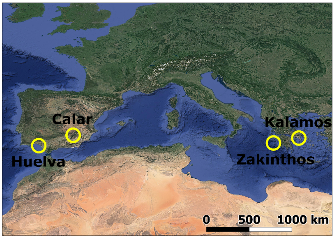
2. Materials
3. Methods
3.1. Ordered Weighted Averaging Operators (OWA)
3.2. Semantics of Ordered Weighted Averaging Operators (OWA)
- Minimum value is obtained when wi = 1 for some i, then dispersion(W) = 0,
- Maximum value is obtained when wi = 1/N for all i, then dispersion(W) = ln(N).
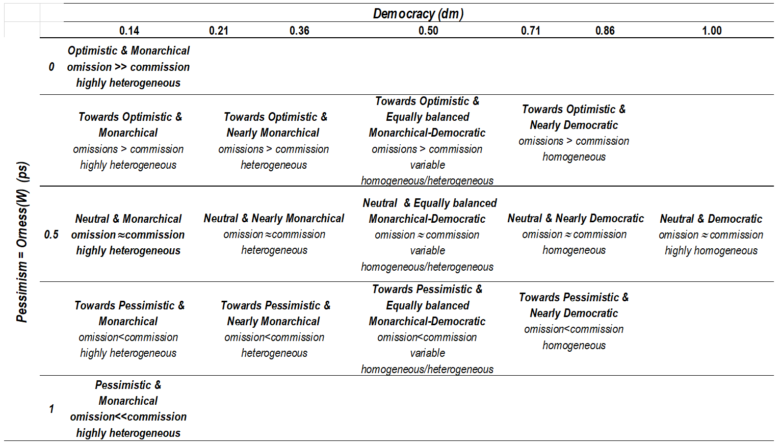
3.3. Fusion Attitude based on Optimism and Democracy
3.4. Learning OWA Weighting Vector from Training Points
…
a1K, ...., aNK → aK
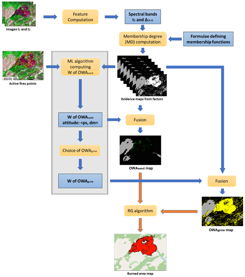
3.5. Workflow of the Automatic BA Mapping Algorithm
If 0.5 ≤ ps ≤ 0.75 then OWAgrow = OWAAverage
If 0.25 ≤ ps < 0.5 then OWAgrow = OWAAlmost_OR
If 0 ≤ ps < 0.25 then OWAgrow = OWAOR
0 < 0.08 < 0.5 < 0.92 < 1
3.6. Validation Metrics
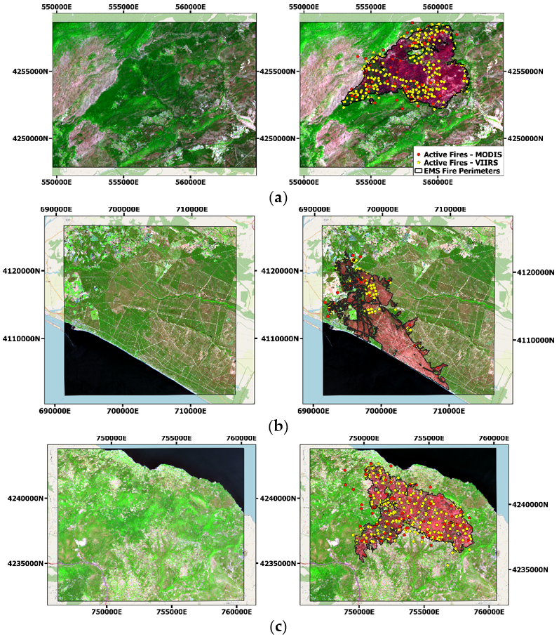
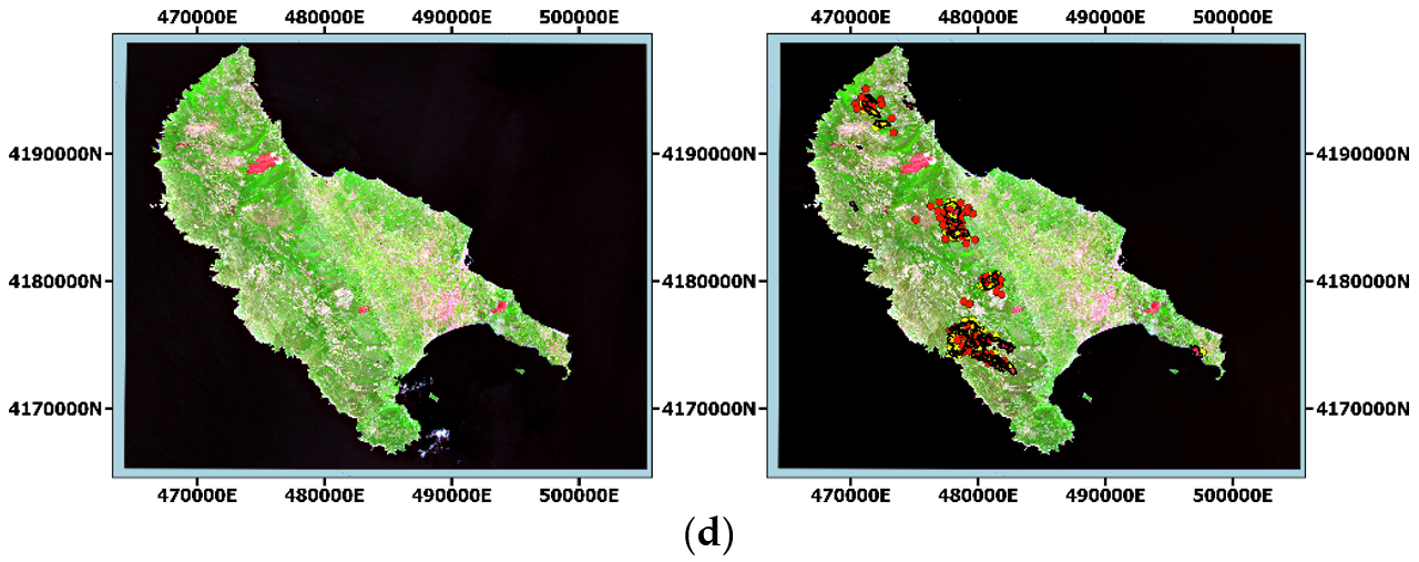
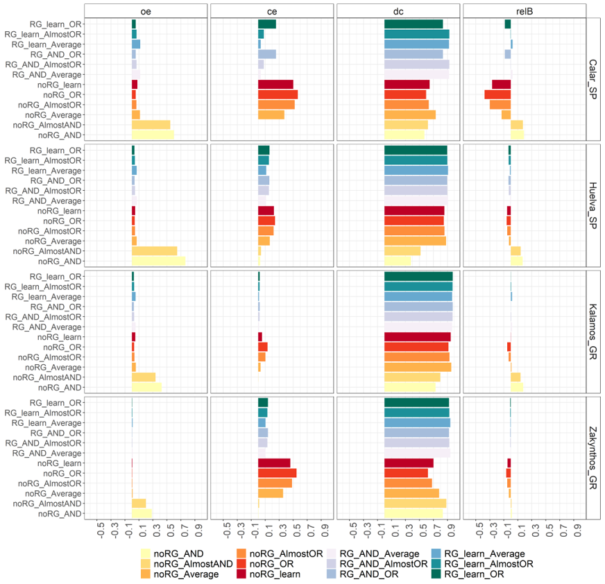
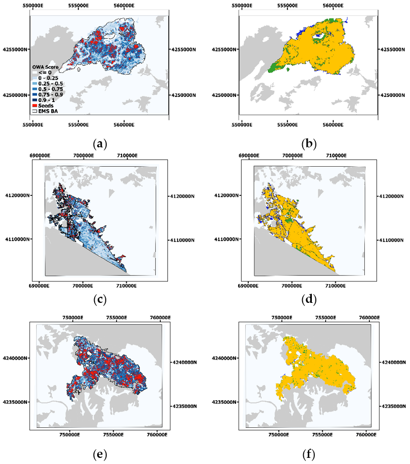
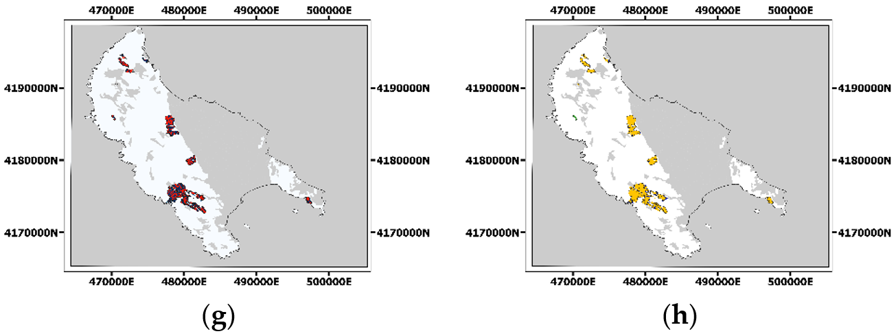
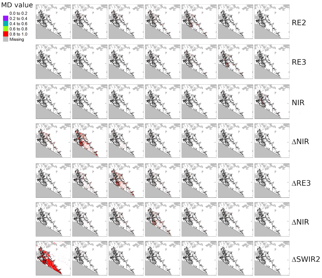
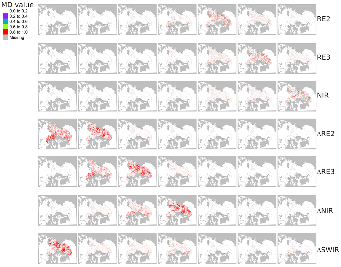
4. Results
4.1. Learning the OWA Operator for Seed Layer Computation
4.2. Burned Area Mapping Accuracy
5. Discussion
6. Conclusions
Author Contributions
Funding
Institutional Review Board Statement
Informed Consent Statement
Data Availability Statement
Acknowledgments
Conflicts of Interest
Appendix A

| Seed | Grow | Label | TP | TN | FP | FN | oe | ce | dc | Relbias |
|---|---|---|---|---|---|---|---|---|---|---|
| Calar SP | ||||||||||
| AND | Average | RG_AND_Average | 282073 | 1005800 | 10195 | 37818 | 0.118 | 0.035 | 0.920 | 0.027 |
| AND | AlmostOR | RG_AND_AlmostOR | 298753 | 990104 | 25891 | 21138 | 0.066 | 0.080 | 0.930 | −0.005 |
| AND | OR | RG_AND_OR | 303087 | 912916 | 103079 | 16804 | 0.053 | 0.254 | 0.830 | −0.085 |
| learn | Average | RG_learn_Average | 282276 | 1005800 | 10195 | 37615 | 0.118 | 0.035 | 0.920 | 0.027 |
| learn | AlmostOR | RG_learn_AlmostOR | 298753 | 990104 | 25891 | 21138 | 0.066 | 0.080 | 0.930 | −0.005 |
| learn | OR | RG_learn_OR | 303087 | 912916 | 103079 | 16804 | 0.053 | 0.254 | 0.830 | −0.085 |
| Average | 0.079 | 0.123 | 0.89 | −0.021 | ||||||
| Standard deviation | 0.031 | 0.103 | 0.05 | 0.052 | ||||||
| Huelva SP | ||||||||||
| AND | Average | RG_AND_Average | 780066 | 3659400 | 98225 | 59952 | 0.071 | 0.112 | 0.910 | −0.010 |
| AND | AlmostOR | RG_AND_AlmostOR | 803771 | 3612717 | 144908 | 36247 | 0.043 | 0.153 | 0.900 | −0.029 |
| AND | OR | RG_AND_OR | 807912 | 3603750 | 153875 | 32106 | 0.038 | 0.160 | 0.900 | −0.032 |
| learn | Average | RG_learn_Average | 782787 | 3656845 | 100780 | 57231 | 0.068 | 0.114 | 0.910 | −0.012 |
| learn | AlmostOR | RG_learn_AlmostOR | 805279 | 3610946 | 146679 | 34739 | 0.041 | 0.154 | 0.900 | −0.030 |
| learn | OR | RG_learn_OR | 809420 | 3601876 | 155749 | 30598 | 0.036 | 0.161 | 0.900 | −0.033 |
| Average | 0.050 | 0.142 | 0.903 | −0.024 | ||||||
| Standard deviation | 0.016 | 0.023 | 0.005 | 0.010 | ||||||
| Kalamos GR | ||||||||||
| AND | Average | RG_AND_Average | 260204 | 654869 | 3010 | 14341 | 0.052 | 0.011 | 0.970 | 0.017 |
| AND | AlmostOR | RG_AND_AlmostOR | 265908 | 652499 | 5380 | 8637 | 0.031 | 0.020 | 0.970 | 0.005 |
| AND | OR | RG_AND_OR | 266987 | 651743 | 6136 | 7558 | 0.028 | 0.022 | 0.970 | 0.002 |
| learn | Average | RG_learn_Average | 260204 | 654869 | 3010 | 14341 | 0.052 | 0.011 | 0.970 | 0.017 |
| learn | AlmostOR | RG_learn_AlmostOR | 265908 | 652499 | 5380 | 8637 | 0.031 | 0.020 | 0.970 | 0.005 |
| learn | OR | RG_learn_OR | 266987 | 651743 | 6136 | 7558 | 0.028 | 0.022 | 0.970 | 0.002 |
| Average | 0.037 | 0.018 | 0.970 | 0.008 | ||||||
| Standard deviation | 0.012 | 0.005 | 0.000 | 0.007 | ||||||
| Zakynthos GR | ||||||||||
| AND | Average | RG_AND_Average | 125635 | 2302900 | 14585 | 1122 | 0.009 | 0.104 | 0.940 | −0.006 |
| AND | AlmostOR | RG_AND_AlmostOR | 126159 | 2298491 | 18994 | 598 | 0.005 | 0.131 | 0.930 | −0.008 |
| AND | OR | RG_AND_OR | 126250 | 2296935 | 20550 | 507 | 0.004 | 0.140 | 0.930 | −0.009 |
| learn | Average | RG_learn_Average | 125635 | 2302900 | 14585 | 1122 | 0.009 | 0.104 | 0.940 | −0.006 |
| learn | AlmostOR | RG_learn_AlmostOR | 126159 | 2298491 | 18994 | 598 | 0.005 | 0.131 | 0.930 | −0.008 |
| learn | OR | RG_learn_OR | 126250 | 2296935 | 20550 | 507 | 0.004 | 0.140 | 0.920 | −0.009 |
| Average | 0.006 | 0.125 | 0.932 | −0.008 | ||||||
| Standard deviation | 0.002 | 0.017 | 0.008 | 0.001 | ||||||
| Global Average of full automatic algorithm over all sites | 0.057 | 0.068 | 0.935 | 0.004 | ||||||
| Global Standard deviation | 0.048 | 0.048 | 0.026 | 0.017 | ||||||
| Global Average of best performing algorithm over all sites | 0.044 | 0.080 | 0.9375 | −0.005 | ||||||
| Global Standard deviation | 0.030 | 0.041 | 0,025 | 0.005 | ||||||
| OWA | Label | TP | TN | FP | FN | oe | ce | dc | Relbias |
|---|---|---|---|---|---|---|---|---|---|
| Calar SP | |||||||||
| AND | noRG_AND | 127865 | 1015964 | 31 | 192026 | 0.600 | 0.000 | 0.570 | 0.189 |
| AlmostAND | noRG_AlmostAND | 144475 | 1015940 | 55 | 175416 | 0.548 | 0.000 | 0.620 | 0.173 |
| Average | noRG_Average | 283576 | 845991 | 170004 | 36315 | 0.114 | 0.375 | 0.730 | −0.132 |
| AlmostOR | noRG_AlmostOR | 299316 | 689234 | 326761 | 20575 | 0.064 | 0.522 | 0.630 | −0.301 |
| OR | noRG_OR | 303032 | 618881 | 397114 | 16859 | 0.053 | 0.567 | 0.590 | −0.374 |
| Average | 0.276 | 0.293 | 0.628 | −0.089 | |||||
| Standard deviation | 0.274 | 0.277 | 0.062 | 0.262 | |||||
| Huelva SP | |||||||||
| AND | noRG_AND | 197050 | 3752055 | 5570 | 642968 | 0.600 | 0.000 | 0.38 | 0.170 |
| AlmostAND | noRG_AlmostAND | 295352 | 3745169 | 12456 | 544666 | 0.548 | 0.000 | 0.51 | 0.142 |
| Average | noRG_Average | 782319 | 3601903 | 155722 | 57699 | 0.114 | 0.375 | 0.88 | −0.026 |
| AlmostOR | noRG_AlmostOR | 803296 | 3530378 | 227247 | 36722 | 0.064 | 0.522 | 0.86 | −0.051 |
| OR | noRG_OR | 807342 | 3501864 | 255761 | 32676 | 0.053 | 0.567 | 0.85 | −0.059 |
| Average | 0.313 | 0.139 | 0.696 | 0.035 | |||||
| Standard deviation | 0.362 | 0.100 | 0.234 | 0.111 | |||||
| Kalamos GR | |||||||||
| AND | noRG_AND | 157782 | 657813 | 66 | 116763 | 0.425 | 0.000 | 0.730 | 0.177 |
| AlmostAND | noRG_AlmostAND | 182066 | 657701 | 178 | 92479 | 0.337 | 0.001 | 0.800 | 0.140 |
| Average | noRG_Average | 259006 | 648900 | 8979 | 15539 | 0.057 | 0.034 | 0.950 | 0.010 |
| AlmostOR | noRG_AlmostOR | 264900 | 627739 | 30140 | 9645 | 0.035 | 0.102 | 0.930 | −0.031 |
| OR | noRG_OR | 265990 | 616726 | 41153 | 8555 | 0.031 | 0.134 | 0.910 | −0.050 |
| Average | 0.177 | 0.054 | 0.864 | 0.049 | |||||
| Standard deviation | 0.189 | 0.061 | 0.095 | 0.103 | |||||
| Zakynthos GR | |||||||||
| AND | noRG_AND | 90652 | 2317245 | 240 | 36105 | 0.285 | 0.003 | 0.830 | 0.015 |
| AlmostAND | noRG_AlmostAND | 101437 | 2316142 | 1343 | 25320 | 0.200 | 0.013 | 0.880 | 0.010 |
| Average | noRG_Average | 125541 | 2248191 | 69294 | 1216 | 0.010 | 0.356 | 0.780 | −0.029 |
| AlmostOR | noRG_AlmostOR | 126152 | 2199065 | 118420 | 605 | 0.005 | 0.484 | 0.680 | −0.051 |
| OR | noRG_OR | 126259 | 2164238 | 153247 | 498 | 0.004 | 0.548 | 0.620 | −0.066 |
| Average | 0.101 | 0.281 | 0.758 | −0.024 | |||||
| Standard deviation | 0.133 | 0.258 | 0.107 | 0.036 | |||||
References
- Velickov, S.; Solomatine, D.P.; Yu, X.; Price, R.K. Application of Data Mining Techniques for Remote Sensing Image Analysis. In Proceedings of the 4-th International Conference on Hydroinformatics, Iowa City, IA, USA, 23–27 July 2000. [Google Scholar]
- Ramo, R.; García, M.; Rodríguez, D.; Chuvieco, E. A data mining approach for global burned area mapping. Int. J. Appl. Earth Obs. Geoinf. 2018, 73, 39–51. [Google Scholar] [CrossRef]
- Quintano, C.; Fernández-Manso, A.; Stein, A.; Bijker, W. Estimation of area burned by forest fires in Mediterranean countries: A remote sensing data mining perspective. For. Ecol. Manag. 2011, 262, 1597–1607. [Google Scholar] [CrossRef]
- Liu, Z.; Peng, C.; Work, T.; Candau, J.-N.; DesRochers, A.; Kneeshaw, D. Application of machine-learning methods in forest ecology: Recent progress and future challenges. Environ. Rev. 2018, 26, 339–350. [Google Scholar] [CrossRef] [Green Version]
- Shen, C. A Transdisciplinary Review of Deep Learning Research and Its Relevance for Water Resources Scientists. Water Resour. Res. 2018, 54, 8558–8593. [Google Scholar] [CrossRef]
- Karpatne, A.; Ebert-Uphoff, I.; Ravela, S.; Babaie, H.A.; Kumar, V. Machine Learning for the Geosciences: Challenges and Opportunities. IEEE Trans. Knowl. Data Eng. 2019, 31, 1544–1554. [Google Scholar] [CrossRef] [Green Version]
- Arif, M.; Alghamdi, K.K.; Sahel, S.A.; Alosaimi, S.O.; Alsahaft, M.E.; Alharthi, M.A.; Arif, M. Role of Machine Learning Algorithms in Forest Fire Management: A Literature Review. J. Robot. Autom. 2021, 5, 212–226. [Google Scholar]
- Sun, A.Y.; Scanlon, B.R. How can Big Data and machine learning benefit environment and water management: A survey of methods, applications, and future directions. Environ. Res. Lett. 2019, 14, 073001. [Google Scholar] [CrossRef]
- Cui, Y.; Chen, X.; Gao, J.; Yan, B.; Tang, G.; Hong, Y. Global water cycle and remote sensing Big data: Overview, challenge, and opportunities. Big Earth Data 2018, 2, 282–297. [Google Scholar] [CrossRef]
- Jain, P.S.; Coogan, C.P.; Subramaniany, S.G.; Crowley, M.; Taylor, S.; Flannigan, M.D. A review of machine learning applications in wildfire science and management. Environ. Rev. 2020, 28, 478–505. [Google Scholar] [CrossRef]
- European Parliament and Council of the European Union. Regulation (EU) 2016/679 of the European Parliament and of the Council of 27 April 2016 on the Protection of Natural Persons with Regard to the Processing of Personal Data and on the Free Movement of Such Data, and Repealing Directive 95/46/EC (General Data Protection Regulation). 2016. Available online: https://op.europa.eu/it/publication-detail/-/publication/3e485e15-11bd-11e6-ba9a-01aa75ed71a1/language-en (accessed on 29 July 2021).
- European Commission. White Paper: On Artificial Intelligence—A European Approach to Excellence and Trust; EU: Brussels, Belgium, 2020; Volume 65, pp. 1–26. [Google Scholar]
- European Commission. High Level Expert Group on Artificial Intelligence 2019. Ethics Guidelines for Trustworthy AI. Available online: https://digital-strategy.ec.europa.eu/en/library/ethics-guidelines-trustworthy-ai (accessed on 29 July 2021).
- Hamon, R.; Junklewitz, H.; Malgieri, G.; De Hert, P.; Beslay, L.; Sanchez, I. Impossible Explanations? Beyond Explainable AI in the GDPR from a COVID-19 Use Case Scenario. In Proceedings of the 2021 ACM Conference on Fairness, Accountability, and Transparency, Virtual Event Canada, Toronto, ON, Canada, 3–10 March 2021; ISBN 9781450383097. [Google Scholar] [CrossRef]
- Emre, B. Transparency of Automated Decisions in the GDPR: An Attempt for Systemisation. SSRN 2018. [Google Scholar] [CrossRef]
- Felzmann, H.; Fosch-Villaronga, E.; Lutz, C.; Tamò-Larrieux, A. Towards Transparency by Design for Artificial Intelligence. Sci. Eng. Ethics 2020, 26, 3333–3361. [Google Scholar] [CrossRef]
- Rudin, C. Stop explaining black box machine learning models for high stakes decisions and use interpretable models instead. Nat. Mach. Intell. 2019, 1, 206–215. [Google Scholar] [CrossRef] [Green Version]
- Yager, R.R. Quantifier guided aggregation using OWA operators. Int. J. Intell. Syst. 1996, 11, 49–73. [Google Scholar] [CrossRef]
- Leblon, B.; Bourgeau-Chavez, L.; San-Miguel-Ayanz, J. Use of Remote Sensing in Wildfire Management. In Sustainable Development, Authoritative and Leading Edge Content for Environmental; Curkovic, S., Ed.; InTech: Rijeka, Croatia, 2012; ISBN 978-953-51-0682-1. [Google Scholar] [CrossRef]
- Giglio, L.; Loboda, T.; Roy, D.P.; Quayle, B.; Justice, C.O. An active-fire based burned area mapping algorithm for the MODIS sensor. Remote. Sens. Environ. 2009, 113, 408–420. [Google Scholar] [CrossRef]
- Schmoldt, D.L. Application of artificial intelligence to risk analysis for forested ecosystems. In Risk Analysis in Forest Management; Gadow, K.L., Ed.; Springer: Berlin/Heidelberg, Germany, 2001; pp. 49–74. [Google Scholar]
- Olden, J.D.; Lawler, J.J.; Poff, N.L. Machine learning methods without tears: A primer for ecologists. Q. Rev. Biol. 2008, 83, 171–193. [Google Scholar] [CrossRef] [Green Version]
- Roy, D.P.; Huang, H.; Boschetti, L.; Giglio, L.; Yan, L.; Zhang, H.H.; Li, Z. Landsat-8 and Sentinel-2 burned area mapping—A combined sensor multi-temporal change detection approach. Remote Sens. Environ. 2019, 231, 111254. [Google Scholar] [CrossRef]
- Drusch, M.; Del Bello, U.; Carlier, S.; Colin, O.; Fernandez, V.; Gascon, F.; Hoersch, B.; Isola, C.; Laberinti, P.; Martimort, P.; et al. Sentinel-2: ESA’s Optical High-Resolution Mission for GMES Operational Services. Remote Sens. Environ. 2012, 120, 25–36. [Google Scholar] [CrossRef]
- Zhang, H.K.; Roy, D.P.; Yan, L.; Li, Z.; Huang, H.; Vermote, E.; Skakun, S.; Roger, J.-C. Characterization of Sentinel-2A and Landsat-8 top of atmosphere, surface, and nadir BRDF adjusted reflectance and NDVI differences. Remote Sens. Environ. 2018, 215, 482–494. [Google Scholar] [CrossRef]
- Gonzalez, R.C.; Woods, R.E. Digital Image Processing, 2nd ed.; Prentice Hall: Hoboken, NJ, USA, 2002. [Google Scholar]
- Espindola, G.M.; Camara, G.; Reis, I.A.; Bins, L.S.; Monteiro, A.M. Parameter selection for region-growing image segmentation algorithms using spatial autocorrelation. Int. J. Remote Sens. 2006, 27, 3035–3040. [Google Scholar] [CrossRef]
- Stroppiana, D.; Bordogna, G.; Carrara, P.; Boschetti, M.; Boschetti, L.; Brivio, P.A. A method for extracting burned areas from Landsat TM/ETM+ images by soft aggregation of multiple Spectral Indices and a region growing algorithm. ISPRS J. Photogramm. Remote Sens. 2012, 69, 88–102. [Google Scholar] [CrossRef]
- Zhang, T.; Yang, X.; Hu, S.; Su, F. Extraction of Coastline in Aquaculture Coast from Multispectral Remote Sensing Images: Object-Based Region Growing Integrating Edge Detection. Remote Sens. 2013, 5, 4470–4487. [Google Scholar] [CrossRef] [Green Version]
- Shan, T.; Wang, C.; Chen, F.; Wu, Q.; Li, B.; Yu, B.; Shirazi, Z.; Lin, Z.; Wu, W. A Burned Area Mapping Algorithm for Chinese FengYun-3 MERSI Satellite Data. Remote Sens. 2017, 9, 736. [Google Scholar] [CrossRef] [Green Version]
- Sali, M.; Piaser, E.; Boschetti, M.; Brivio, P.A.; Sona, G.; Bordogna, G.; Stroppiana, D. A Burned Area Mapping Algorithm for Sentinel-2 Data Based on Approximate Reasoning and Region Growing. Remote Sens. 2021, 13, 2214. [Google Scholar] [CrossRef]
- Goffi, A.; Bordogna, G.; Stroppiana, D.; Boschetti, M.; Brivio, P.A. Knowledge and Data-Driven Mapping of Environmental Status Indicators from Remote Sensing and VGI. Remote Sens. 2020, 12, 495. [Google Scholar] [CrossRef] [Green Version]
- Sánchez-Benítez, A.; García-Herrera, R.; Barriopedro, D.; Sousa, P.M.; Trigo, R.M. June 2017: The Earliest European Summer Mega-heatwave of Reanalysis Period. Geophys. Res. Lett. 2018, 45, 1955–1962. [Google Scholar] [CrossRef]
- Turco, M.; Jerez, S.; Augusto, S.; Tarin-Carrasco, P.; Ratola, N.; Jimenez-Guerrero, P.; Trigo, R.M. Climate drivers of the 2017 devastating fires in Portugal. Sci. Rep. 2019, 9, 13886. [Google Scholar] [CrossRef]
- Available online: https://earth.esa.int/web/sentinel/home (accessed on 29 July 2021).
- Sali, M.; Busetto, L.; Boschetti, M.; Franquesa, M.; Chuvieco, E.; Stroppiana, D. Fire Reference Perimeters Extracted from Sentinel-2 Data for Validation of Burned Area Products in Africa Biomes. In Proceedings of the IGARSS 2021 IEEE International Geoscience and Remote Sensing Symposium, Brussels, Belgium, 11–16 July 2021; pp. 3749–3752. [Google Scholar]
- Available online: https://scihub.copernicus.eu/ (accessed on 29 July 2021).
- Ranghetti, L.; Busetto, L. Sen2r: An R toolbox to find, download and preprocess Sentinel-2 data. R Package Version. 2019. Available online: https://zenodo.org/record/5035912#.YRX4wnkRXIU (accessed on 29 July 2021).
- Available online: https://ranghetti.github.io/sen2r (accessed on 29 July 2021).
- Available online: https://land.copernicus.eu/global/products/ba (accessed on 29 July 2021).
- Giglio, L.; Schroeder, W.; Justice, C.O. The Collection 6 MODIS active fire detection algorithm and fire products. Remote Sens. Environ. 2016, 178, 31–41. [Google Scholar] [CrossRef] [Green Version]
- Schroeder, W.; Oliva, P.; Giglio, L.; Csiszar, I.A. The New VIIRS 375m active fire detection data product: Algorithm description and initial assessment. Remote Sens. Environ. 2014, 143, 85–96. [Google Scholar] [CrossRef]
- Robinson, P.B. A perspective on the fundamentals of fuzzy sets and their use in geographic information systems. Trans. GIS 2003, 7, 3–30. [Google Scholar] [CrossRef]
- Carrara, P.; Bordogna, G.; Boschetti, M.; Brivio, P.A.; Nelson, A.; Stroppiana, D. A flexible multi-source spatial-data fusion system for environmental status assessment at continental scale. Int. J. Geogr. Inf. Sci. 2008, 22, 781–799. [Google Scholar] [CrossRef]
- Stroppiana, D.; Boschetti, M.; Zaffaroni, P.; Brivio, P.A. Analysis and interpretation of spectral indices for soft multi-criteria burned area mapping in Mediterranean regions. IEEE Geosci. Remote. Sens. Lett. 2009, 6, 499–503. [Google Scholar] [CrossRef]
- Yager, R.R. On ordered weighted averaging aggregation operators in multi-criteria decision making. IEEE Trans. on Syst. Man Cybern. 1998, 18, 183–190. [Google Scholar] [CrossRef]
- Marichal, J.L. Tolerant or intolerant character of interacting criteria in aggregation by the Choquet integral. Eur. J. Oper. Res. 2004, 155, 771–791. [Google Scholar] [CrossRef] [Green Version]
- Bordogna, G.; Pagani, M.; Pasi, G. A Flexible Decision support approach to model ill-defined knowledge in GIS. In Proceedings of the NATO Workshop on Environmental Impact Assement, Kiew, Ukraine, 23–26 June 2006. [Google Scholar]
- Yager, R.R. New modes of OWA information fusion. Int. J. Intell. Syst. 1998, 13, 661–681. [Google Scholar] [CrossRef]
- Yager, R.R. On the dispersion measure of OWA operators. Inf. Sci. 2009, 179, 3908–3919. [Google Scholar] [CrossRef]
- Congalton, R.G. Accuracy assessment and validation of remotely sensed and other spatial information. Int. J. Wildland Fire 2001, 10, 321–328. [Google Scholar] [CrossRef] [Green Version]
- Chicco, D.; Jurman, G. The advantages of the Matthews correlation coefficient (MCC) over F1 score and accuracy in binary classification evaluation. BMC Genom. 2020, 21, 6. [Google Scholar] [CrossRef] [Green Version]
- Stehman, S.V. Selecting and Interpreting Measures of Thematic Classification Accuracy. Remote Sens. Environ. 1997, 62, 77–89. [Google Scholar] [CrossRef]
- Stehman, S.V.; Czaplewski, R.L. Design and Analysis for Thematic Map Accuracy Assessment: Fundamental Principles. Remote Sens. Environ. 1998, 64, 331–344. [Google Scholar] [CrossRef]
- Padilla, M.; Stehman, S.V.; Hantson, S.; Oliva, P.; Alonso-Canas, I.; Bradley, A.; Tansey, K.; Mota, B.; Pereira, J.M.; Chuvieco, E. Comparing the Accuracies of Remote Sensing Global Burned Area Products using Stratified Random Sampling and Estimation. Remote Sens. Environ. 2015, 160, 114–121. [Google Scholar] [CrossRef] [Green Version]
- Fernandez-Carrillo, A.; Franco-Nieto, A.; Pinto-Bañuls, E.; Basarte-Mena, M.; Revilla-Romero, B. Designing a Validation Protocol for Remote Sensing Based Operational Forest Masks Applications. Comparison of Products Across Europe. Remote Sens. 2020, 12, 3159. [Google Scholar] [CrossRef]
- Dice, L.R. Measures of the amount of ecologic association between species. Ecology 1945, 26, 297–302. [Google Scholar] [CrossRef]
- CLC. 2012. Available online: https://land.copernicus.eu/pan-european/corine-land-cover (accessed on 29 July 2021).
- Bastarrika, A.; Chuvieco, E.; Martín, M.P. Mapping burned areas from Landsat TM/ETM+ data with a two-phase algorithm: Balancing omission and commission errors. Remote Sens. Environ. 2011, 115, 1003–1012. [Google Scholar] [CrossRef]
- Wu, L.; Wang, Y.; Long, J.; Liu, Z. A Non-seed-based Region Growing Algorithm for High Resolution Remote Sensing Image Segmentation. In Image and Graphics; Zhang, Y.J., Ed.; Springer: Berlin/Heidelberg, Germany, 2015. [Google Scholar] [CrossRef] [Green Version]
- Li, Z.; Kaufman, Y.J.; Ichoku, C.; Fraser, R.; Trishchenke, A.; Giglio, L.; Jin, J.; Yu, X. A review of AVHRR-based active fire detection algorithms: Principles, limitations, and recommendations. In Global and Regional Vegetation Fire Monitoring from Space. Planning a Coordinated and International Effort; Ahern, F.J., Goldammer, J.G., Justice, C.O., Eds.; SPB Academic: The Hague, The Netherlands, 2001; pp. 199–225. [Google Scholar]
- Roy, D.P.; Landmann, T. Characterising the surface heterogeneity of fire effects using multi temporal reflecting wavelength data. Int. J. Remote Sens. 2005, 26, 4197–4218. [Google Scholar] [CrossRef]
- Boschetti, L.; Brivio, P.A.; Eva, H.D.; Gallego, J.; Baraldi, A.; Gregoire, J.-M. A sampling method for the retrospective validation of global burned area products. IEEE Trans. Geosci. Remote Sens. 2006, 44, 1765–1773. [Google Scholar] [CrossRef]
- Pulvirenti, L.; Squicciarino, G.; Fiori, E.; Fiorucci, P.; Ferraris, L.; Negro, D.; Gollini, A.; Severino, M.; Puca, S. An Automatic Processing Chain for Near Real-Time Mapping of Burned Forest Areas Using Sentinel-2 Data. Remote Sens. 2020, 12, 674. [Google Scholar] [CrossRef] [Green Version]
- Smiraglia, D.; Filipponi, F.; Mandrone, S.; Tornato, A.; Taramelli, A. Agreement Index for Burned Area Mapping: Integration of Multiple Spectral Indices Using Sentinel-2 Satellite Images. Remote Sens. 2020, 12, 1862. [Google Scholar] [CrossRef]
- Seydi, S.T.; Akhoondzadeh, M.; Amani, M.; Mahdavi, S. Wildfire Damage Assessment over Australia Using Sentinel-2 Imagery and MODIS Land Cover Product within the Google Earth Engine Cloud Platform. Remote Sens. 2021, 13, 220. [Google Scholar] [CrossRef]


| Band Name | Spectral Domain | Central Wavelength (µm) | Spatial Resolution [m] | Features Name |
|---|---|---|---|---|
| Band 2 | Blue | 0.490 | 10 | RE2 and ΔRE2 |
| Band 3 | Green | 0.560 | 10 | RE2 and ΔRE2 |
| Band 4 | Red | 0.665 | 10 | Red and ΔRed |
| Band 5 | Red Edge 1 | 0.705 | 20 | RE1 and ΔRE1 |
| Band 6 | Red Edge 2 | 0.740 | 20 | RE2 and ΔRE2 |
| Band 7 | Red Edge 3 | 0.783 | 20 | RE3 and ΔRE3 |
| Band 8 | NIR | 0.842 | 10 | NIR and ΔNIR |
| Band 11 | SWIR 1 | 1.610 | 20 | SWIR1 and ΔSWIR1 |
| Band 12 | SWIR 2 | 2.190 | 20 | SWIR2 and ΔSWIR2 |
| Study Site | Pre-Fire Date | Post-fire Date | Reference Date |
|---|---|---|---|
| Calar, Spain | 15/07 | 04/08 | 04/08 |
| Huelva, Spain | 11/06 | 01/07 | 27/06 |
| Zakynthos, Greece | 25/07 | 03/09 | 18/08 |
| Kalamos, Greece | 28/07 | 17/08 | 18/08 |
| EMS Reference | ||||
|---|---|---|---|---|
| Burned | Unburned | Total | ||
| RG algorithm | Burned | n11 | n12 | n1+ |
| Unburned | n21 | n22 | n2+ | |
| Total | n+1 | n+2 | ||
| Accuracy Metric Name | Formula | Range |
|---|---|---|
| Commission error | [0, 1] | |
| Omission Error | [0, 1] | |
| Dice Coefficient | [0, 1] | |
| Relative Bias | [−1, +1] |
| OWAlearn Weighting Vector | ps | dm | Attitude | Expected Errors in Seed Layer | Predicted OWAgrow (OWAseed = OWAlearn) | Best OWAgrow (OWAseed = AND) | |
|---|---|---|---|---|---|---|---|
| Calar | [0.43, 0.02, 0.03, 0.03, 0.13, 0.16, 0.21, 0.55, 0.67] | 0.55 | 0.67 | Towards Pessimistic and Nearly Democratic | ce ≥ oe | Average | Almost OR (Δdc = 0.01) |
| Huelva | [0.69, 0.00, 0.00, 0.00, 0.00, 0.00, 0.30, 0.70, 0.28] | 0.70 | 0.28 | Towards Pessimistic and Nearly Monarchical | ce > oe | Average | Average |
| Kalamos | [0.36, 0.02, 0.00, 0.00, 0.02, 0.11, 0.49, 0.4, 0.45] | 0.40 | 0.45 | Towards Optimistic and Nearly Monarchical | oe ≥ ce | Almost OR | OR (Δdc = 0.007) |
| Zakynthos | [0.53, 0.00, 0.00, 0.00, 0.00, 0.00, 0.46, 0.5, 0.30] | 0.54 | 0.30 | Towards Pessimistic and Nearly Monarchical | ce ≥ oe | Average | Average |
Publisher’s Note: MDPI stays neutral with regard to jurisdictional claims in published maps and institutional affiliations. |
© 2021 by the authors. Licensee MDPI, Basel, Switzerland. This article is an open access article distributed under the terms and conditions of the Creative Commons Attribution (CC BY) license (https://creativecommons.org/licenses/by/4.0/).
Share and Cite
Stroppiana, D.; Bordogna, G.; Sali, M.; Boschetti, M.; Sona, G.; Brivio, P.A. A Fully Automatic, Interpretable and Adaptive Machine Learning Approach to Map Burned Area from Remote Sensing. ISPRS Int. J. Geo-Inf. 2021, 10, 546. https://0-doi-org.brum.beds.ac.uk/10.3390/ijgi10080546
Stroppiana D, Bordogna G, Sali M, Boschetti M, Sona G, Brivio PA. A Fully Automatic, Interpretable and Adaptive Machine Learning Approach to Map Burned Area from Remote Sensing. ISPRS International Journal of Geo-Information. 2021; 10(8):546. https://0-doi-org.brum.beds.ac.uk/10.3390/ijgi10080546
Chicago/Turabian StyleStroppiana, Daniela, Gloria Bordogna, Matteo Sali, Mirco Boschetti, Giovanna Sona, and Pietro Alessandro Brivio. 2021. "A Fully Automatic, Interpretable and Adaptive Machine Learning Approach to Map Burned Area from Remote Sensing" ISPRS International Journal of Geo-Information 10, no. 8: 546. https://0-doi-org.brum.beds.ac.uk/10.3390/ijgi10080546