The Integration of Linguistic and Geospatial Features Using Global Context Embedding for Automated Text Geocoding

Abstract

Geocoding is an essential procedure in geographical information retrieval to associate place names with coordinates. Due to the inherent ambiguity of place names in natural language and the scarcity of place names in textual data, it is widely recognized that geocoding is challenging. Recent advances in deep learning have promoted the use of the neural network to improve the performance of geocoding. However, most of the existing approaches consider only the local context, e.g., neighboring words in a sentence, as opposed to the global context, e.g., the topic of the document. Lack of global information may have a severe impact on the robustness of the model. To fill the research gap, this paper proposes a novel global context embedding approach to generate linguistic and geospatial features through topic embedding and location embedding, respectively. A deep neural network called LGGeoCoder, which integrates local and global features, is developed to solve the geocoding as a classification problem. The experiments on a Wikipedia place name dataset demonstrate that LGGeoCoder achieves competitive performance compared with state-of-the-art models. Furthermore, the effect of introducing global linguistic and geospatial features in geocoding to alleviate the ambiguity and scarcity problem is discussed.

1. Introduction

Web and smartphone technologies have brought vast volumes of unstructured text information to the Web, which has gradually changed people’s needs for searching information, leading to changes in search services. The function of adding geographic information from web resources (e.g., texts) to Geographic Information Retrieval (GIR) and indexing it has become notably attractive [1]. For example, the location information in social media data could be tracked for poll analysis [2] or delineating activity spaces [3]. Geoparsing is a procedure to detect the geographic information in texts and link with gazetteers, a database storing place names and their attributes, including coordinates, population, size, and type [4]. This process generally involves geotagging that recognizes place names in text and geocoding that transforms place names into coordinates [5,6,7]. Geotagging commonly recognizes place names in a text by constructing geographical language models trained on massive corpora of geotagged annotations, such as river, city, etc. [8]. The goal of geocoding is to select the correct coordinate for the place name from a list of candidate coordinates from a gazetteer such as GeoNames [9]. The common pipeline of geocoding is to disambiguate the place names first and then link the gazetteer [5].

This article concentrates on addressing the ambiguity of place names, the non-trivial issue of the geocoding [10,11,12]. The place name disambiguation needs to deal with two levels of ambiguity, including linguistics and geography. For linguistics, due to the inherent ambiguity of natural language, place names often have other non-geographic meanings and different locations are referred to as the same name. For geography, the ambiguity is the vague of location information in place names. For example, it is unclear what is the range specified by saying “the bank of a river”. Disambiguation is widely studied in Natural Language Processing (NLP) to distinguish the semantic and syntactic structure in the context [13]. However, it is difficult to obtain the complete context of place names in the geocoding problem due to the lack of geographical location information in natural language. For instance, considering the following two sentences containing “Washington”.

Washington is a census-designated place located in Nevada County, California.

Washington is located on the bank of the South Fork of the Yuba River.

Without knowing the location of Yuba River, it is impossible to determine whether those two sentences are related and distinguish the two “Washington” words.

One feasible solution is to introduce extra information from gazetteers. Presently, many approaches apply machine learning to solve geocoding [6]. Recent research demonstrates that using feature representation and gazetteers to express the geographical distribution of place mentions, and integrating them into linguistic features can improve the performance of geocoding [14]. However, the limitation of the methods mentioned above is that the extracted linguistic features and geospatial features are limited to the co-occurrence of words or location information in a text, which could not summarize the full features of the location. In other words, these methods only extract local context but not global context. The global context is inherent co-occurrence patterns or clustering structures between different texts. For example, the global context can be regarded as a set of sentences that describe the same characteristics and have a common topic in natural language. Lack of the ability to collect global contextual information increases the chance of misclassification.

This paper proposes to use two global context embedding methods, including topic embedding and location embedding for linguistic and geospatial feature extraction, respectively. Subsequently, a novel neural network named LGGeoCoder is designed for geocoding to integrate multiple forms of features, including local and global features, linguistic and geographic features. The global context embedding are used to extract features in an unsupervised manner. From this perspective, our global features are obtained from unlabeled samples. The overall architecture of LGGeoCoder is inspired using pre-training techniques in NLP to deal with data scarcity [15]. Our extensive evaluation of the Wikipedia place names database published by [14] shows the method achieves competitive performance compared with the state-of-the-art method.

The main contributions of the paper include the following three points:

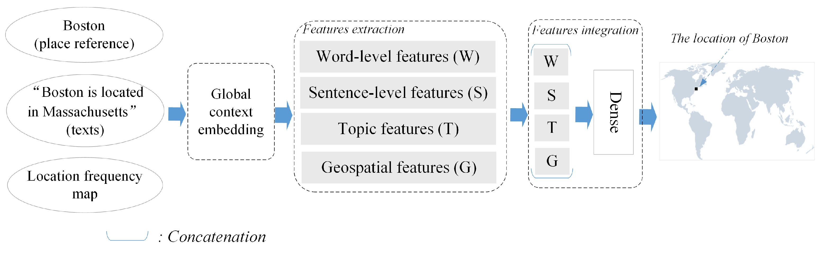
• It employs topic embedding to improve feature representation by enforcing topic modeling to transform words’ topics into low-dimensional vectors. However, traditional geocoding tasks ignore topic information and are limited to the syntax and semantics of text.
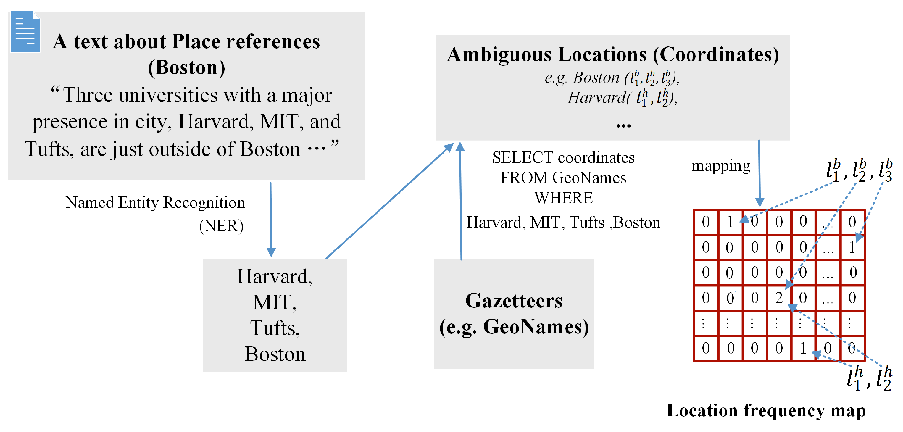
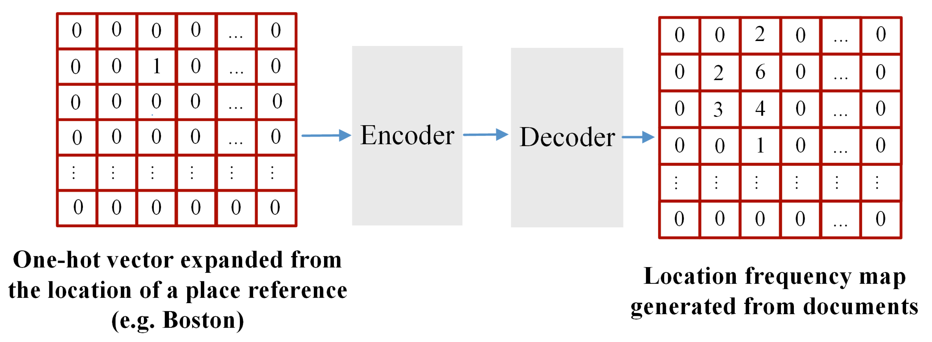
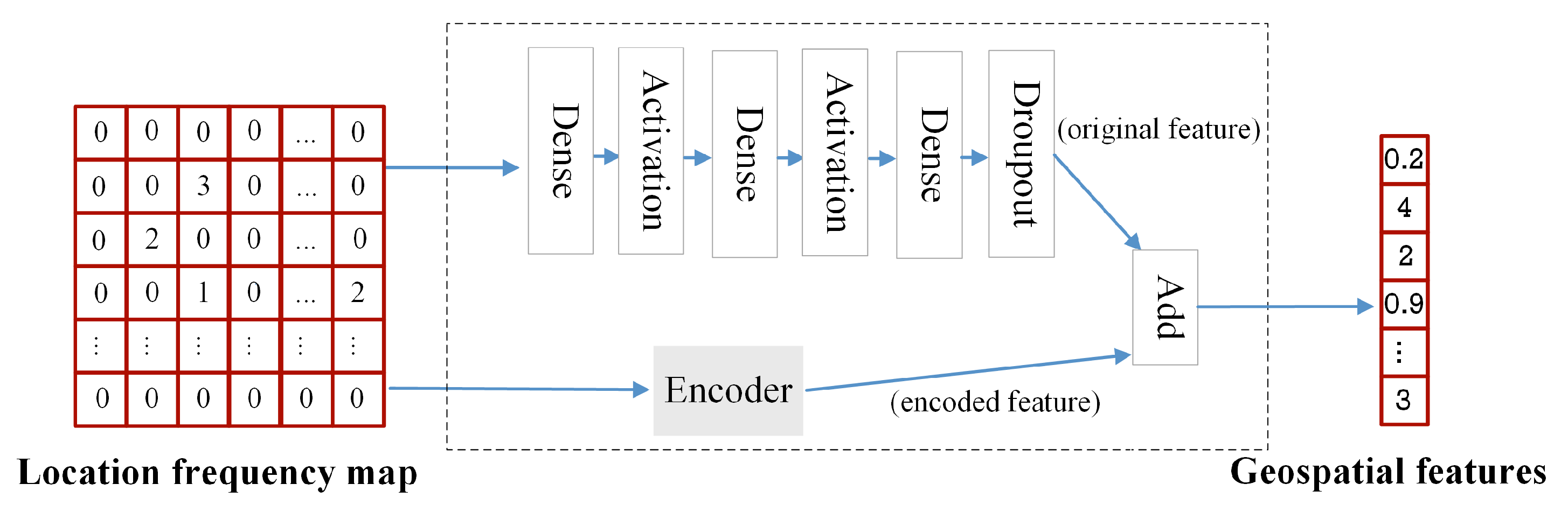
• It employs location embedding from deep learning to transform spatial distribution around the place reference into low-dimensional vectors and enrich the geospatial features vector. Since place mentions in a text are often few, the location embedding works as a priori feature aiding the generation of the geospatial feature vector to alleviate the data scarcity.
• It discovers that fusion with topic information can effectively reduce the geospatial feature vector’s noise.

The remainder of this article is organized as follows. Section 2 introduces related work. Section 3 presents the proposed method in detail. The effectiveness of the proposed method is demonstrated by experiments in Section 4. Finally, Section 5 presents conclusions and future work.

2. Related Work

In traditional GIS, the term geocoding often means address geocoding, which aims to convert a postal address into geographic coordinates [16]. With the emergence of large amounts of text, the term geocoding is enriched with NLP [5,17]. It can be treated as special cases of Named Entity Disambiguation (NED) [5,6,18]. Moreover, it draws extensively on ideas from NED [6].

The methods of geocoding can be divided into two categories, rule-based and data-driven methods. Rule-based methods often use clues of text contexts as rules to eliminate place name ambiguity [19]. These clues could be characteristics of the place names, such as population [17], word frequency [20], types [21], and spatial relations between places [22]. The rule-based methods are often interpretative yet are limited in dealing with unstructured data. For example, social media data often omits administrative characteristics of place names, which may lead to methods unable to use rules in disambiguation. Recent research gradually shifted from rule-based methods to data-driven methods, which use statistical and machine learning approaches to deal with the local context [6]. Statistical methods [23] usually face high computational complexity, and some approximate calculation assumptions are often put forward, which usually loses a lot of information. With the exponential growth of the Internet community and the emergence of a large amount of text, researchers are increasingly inclined to let machines automatically obtain features, leading to research focusing on the use of machine learning methods.

According to the label of the training sample, machine learning can be divided into supervised learning, unsupervised learning and, semi-supervised learning [24]. Supervised learning requires labels to be able to train the model, which can often achieve good results when used in geocoding. For example, geocoding can be improved based on the text using a hierarchy of logistic regression classifiers [25], a Support Vector Machine (SVM) algorithm [26]. In 2015, deep learning methods were also proven to help improve geocoding performance [27]. However, supervised methods heavily rely on the availability of sense-annotated corpora. Because on a corpus with data scarcity supervised methods can lead to overfitting [24], they are unsuitable for processing large corpus. Some research suggests that semi-supervised methods can solve overfitting in geocoding by introducing unsupervised methods [12,28,29,30] to further learn unlabeled data [6,31]. In the field of machine learning, this approach is also called unsupervised pre-training.

In 2013, the word2vec algorithm combined with unsupervised pre-training was proposed to process NLP tasks [32]; it shows better performance and gains extensive attention. The main contribution is the introduction of a word embedding model based on word similarity to encode the feature space of word meaning into a low-dimensional vector space. The rationale of word2vec was quickly applied to the geospatial domain, capturing the similarity of place names by dividing geographic locations into different regions [33] or dividing geographic locations by popular place names [34] to express geographic spatial features. However, these models only consider the local context and do not consider global context. The global context can effectively promote word sense disambiguation [35]. Our work focuses on designing an embedding method for geospatial feature extraction, which can be reasonably introduced into geocoding through unsupervised pre-training to facilitate the dynamic acquisition of global context information.

3. Methodology

In this section, we provide the methodology of the paper. In Section 3.1, we give the mathematical definition of the geocoding and the definition of the location frequency map, which is used to extract geospatial features. The global context embedding and the framework of LGGeoCoder are introduced in Section 3.2 and Section 3.3, respectively.

3.1. Preliminaries

In geocoding, a deep learning algorithm is designed to classify place names as locations on a map. Our algorithm also considers two data sources, including documents and gazetteer, and extract linguistic features and geospatial features separately. Specifically, given some texts (D) in documents and a set of locations (G) derived from gazetteer and related to the text, the task is to resolve to the location of place reference, which is denoted by x. Then, the problem can be expressed as finding a conditional distribution.

$$P\left(x\right|D,G)$$

(1)

Before computing the conditional probability in Equation (1), the rough boundary for the locations of place names is defined. Here the surface of the earth is partitioned into a grid space, and each location x is represented by a grid cell. In the experiment, we used a cell with a resolution of 1 × 1 degree (1 degree on the equator is about 111 km). Frequency information of location references in a sentence is collected and stores in a map, which is called a location frequency map. Specifically, a NER tool developed by Spacy [36], is first used to obtain the place names of texts. Then, the place names are matched with a gazetteer to retrieve the corresponding ambiguous coordinates. At last, a location frequency map is generated by mapping the ambiguous coordinates of a text to the cells, where the value of cells is the frequency of place names. Figure 1 shows how to generate a location frequency map from a text.

3.2. Global Context Embedding for Linguistic Features and Geospatial Features

This section mainly explains how to construct the global context embedding methods. First, local linguistic feature extraction with word embedding is introduced, and then how to employ topic embedding to obtain global linguistic features is explained. Finally, how to employ location embedding to construct a geospatial feature extraction network with global features is described.

3.2.1. Word Embedding for Linguistic Features

The features here are extracted from the local context, which refers to various combinations of words in distinguishing the place references. It addresses both semantics and syntax of texts and is also known as a component-based grammar [37]. For example, consider the following sentences where the word “New York” is a place reference, “New York is a settlement in Nidderdale in the Harrogate district of North Yorkshire, England.” The context of “New York” contains important semantics, such as “Nidderdale”, “Harrogate district of North Yorkshire”, “England” and vocabularies that are related to places, such as “settlement”. The combination of some words such as “in Nidderdale in the Harrogate district of North Yorkshire” implies relevant properties of the place reference. Two modules, including word-level feature extraction and sentence-level feature extraction, are designed to characterize the features. Word-level feature extraction is used to emphasize the characteristics of individual word inside the place reference (e.g., “New” and “York”). Sentence-level features indicate local context.

To extract the word-level and sentence-level features, a word embedding procedure developed by Glove [38] is adopted. It can transform a high dimensional word vector into a low dimensional embedding vector where two similar words are close in the vector space. For instance, “college” and “university” are similar because they have common neighboring words in their context. The similarity of two words is measured by the frequencies of their neighbouring words.

Specifically, the Glove stores the word frequency according to a corpus by constructing a co-occurrence matrix X. The co-occurrence matrix counts the frequency that two words $W_i$ and $W_j$ appear together in a context window, denoted as $X_{i,j}$. For example, when the window size is 1, and $W_{i-1}$ and $W_{i+1}$ are the contextual words of $W_i$. The co-occurrence matrix is to count the number of occurrences of $(W_{i-1},W_i)$ and $(W_i,W_{i+1})$. Then, the Glove captures the importance of the words in different contexts to find similar features of the words by maximizing a cost function, as follows:

$$J\left(D\right)=\sum _{i,j=1}^{V}f\left(X_{i,j}\right)(w_i^T{w}_j+b_i+b_j-log\left(X_{i,j}\right))$$

(2)

where D is a word sequence, V denotes the size of a corpus, f is the weighting function, $w_i,w_j\in R^d$ are word vectors, $b_i$, $b_j\in R$ are bias for $w_i,w_j$ respectively.

3.2.2. Topic Embedding for Global Linguistic Features

The features here are extracted from the global context, which refers to topics of texts in distinguishing the place references. Taking the following sentence as an example, “Boston is considered to be a global pioneer in innovation and entrepreneurship”. The main topic of this sentence is the leading position of Boston’s education in the world. Therefore, “Boston” in this sentence is more likely to link with the coordinate of Boston, Massachusetts. A topic embedding procedure developed by Topical Word Embedding (TWE) [35] is adopted to extract the features.

The main difference from the word embedding is that the TWE considers the correlation among contexts when transforming a high-dimensional word vector into a low-dimensional embedding vector where words are coupled by topics, not isolated. For example, In topic embedding, the word vector of Washington (name) is close to the vector related to the person’s name, and the word vector of Washington, D.C. is close to the vector related to the place name. The generation of TWE consists of two steps. First, Latent Dirichlet Allocation (LDA) [39] is used to get topics of words. In LDA, documents with similar topics are close to each other. Secondly, the topic of each word is generated as a vector using the skip-gram of word2vec [32]. The cost function of TWE, as follows:

$$J\left(D\right)=\sum _{i=1}^V\sum _{-k\le c\le k}logP(w_i,z_i|(w_{i+c},z_{i+c};w_{\Theta }^z))$$

(3)

where V denotes the size of a corpus, k is the context window size of a target word, $w_i$ is the word vector obtained by word embedding, $z_i$ is the topic vector of target word, $w_{\Theta }^z$ is the parameter of the model and the output vector.

3.2.3. Location Embedding for Geospatial Features

The features refer to geospatial relations such as multiple locations containing topological information among themselves and the spatial proximity. The features are implicit in sentences describing place names or carried on explicitly through a coordinate position. Location frequency maps are used as input for the feature extraction. The idea is provided by the CamCoder [14] as an initial investigation, where the assumption to keep multiplicity disregarding grammar and word order is reasonable for multiple place names in sentences. However, the number of place names in a sentence is often limited. Their locations retrieved from a gazetteer are often ambiguous, so that the location frequency maps are very sparse and noisy. As the resolution of the geodetic grid increases, the location frequency maps will become sparser and noisier, which often results in overfitting according to the theory of machine learning (the curse of dimensionality). For this reason, location embedding is used to introduce global context information to overcome these issues.

Since dealing with place names ambiguity is the goal of task, we cannot explicitly use place names to retrieve vectors such as the word embedding. We turned to express locations in the form of probability and redesigned the network structure that introduced the embedding model according to the form of the location frequency maps. The auto-encoder [40,41], a generative network, is used to create an embedding model. The generative network is obtained by solving the prior distribution [24,42], so the location has a rough boundary defined by the prior distribution instead of the previously separated grid boundary. With this advantage, some blank cells in the grid can be adaptively interpolated to obtain an appropriate score to distinguish ambiguity. For example, given a sentence about Washington, “Washington is the county seat of Wilkes County, Georgia, United States.”. When the geocoding is performed, the location embedding can outline the rough boundary of the Georgia state, therefore increasing the prediction probability of the location of Washington in Georgia. Specifically, the method in this paper characterizes geospatial features in the following three steps.

First, the location frequency maps generated from documents are proposed as the global context to enable location embedding. The place names used to generate a location frequency map come from all documents corresponding to place reference.

Next, the auto-encoder is used to create the generation process from the locations of place references to the location frequency maps generated from documents (Figure 2). In essence, it is expected that the deep neural network can facilitate the model learn the cluster boundaries of different locations by capturing the similarity in the corresponding global context. Then an encoder can be generated by embedding geospatial information from documents. The encoder can use low dimensions to represent high-dimensional features to facilitate feature fusion. On the other hand, this feature is a global feature, and introducing it into geocoding can strengthen geospatial features and reduce sparsity.

After obtaining the encoder, the algorithm can use the additional function to fuse encoded features with the original features in location frequency maps (Figure 3). In this way, the encoder facilitates strengthening the information of each location in the location frequency maps. The final network for deriving geospatial features can be formalized in Equation (4).

$$g=\delta (\sum _n{a}_{encoded}^{l-1}\times w_{encoded}^l+b_{encoded}^l)+\delta (\sum _n{a}_{original}^{l-1}\ast w_{original}^l+b_{original}^l)$$

(4)

where $\delta$ represents an activation function, l represents the l-th layer of the network, n represents the number of layers, w denotes the learnable weights, b denotes the learnable bias, $a_{encoded}^{l-1}$ and $a_{original}^{l-1}$ represent dense layers, and both $a_{encoded}^1$ and $a_{original}^1$ are the same, which is a location frequency map. All values of $w_{encoded}^l$ and $b_{encoded}^l$, come from the auto-encoder, which is frozen in the training of geocoding in Figure 3. However, $w_{original}^l$ and $b_{original}^l$ are parameters that are learned from the training of geocoding.

3.2.4. Training of Embedding Model

The embedding model is trained separately. The parameters of the embedding model are fixed when used for the supervised classification. According to the theoretical foundation from [43], word embedding, topic embedding, and location embedding can be seen as regularizers. The loss function is shown in Equation (5). The regularizers can facilitate obtaining a more robust model by modifying the learning algorithm to reduce its generalization error. Furthermore, the model can be much easier to be trained, and geospatial features can play a more effective role in overall features.

$$\begin{array}{cc}\hfill L\left(D\right)=& \sum _{i\in \zeta }l(y_i,f(p_i,s_i))+{\lambda }_1\sum _{i,j}logP\left(w_i\right|w_{i+c})+{\lambda }_2\sum _{i,j}logP\left(t_i\right|t_{i+c})+\hfill \\ \hfill & {\lambda }_3\sum _{i,j}logP\left(g_i\right|g_{i+c})\hfill \end{array}$$

(5)

where $l(y_i,f(p_i,s_i))$ is the object function of the supervised classification model, $s_i$ represents the sample of text, $p_i$ is the place name, $y_i$ is the labelled cell, $\zeta$ represents all geographic cells, ${\lambda }_i$ is a hyperparameter used to adjust the effects of different features, ${\sum }_{i,j}logP\left(w_i\right|w_{i+c})$ is the object function of word embedding, ${\sum }_{i,j}logP\left(t_i\right|t_{i+c})$ is the object function of document embedding, ${\sum }_{i,j}logP\left(g_i\right|g_{i+c})$ is the object function of network embedding, $g_{i+c}$ is the location context of $g_i$.

3.3. LGGeoCoder

The proposed framework consists of input, linguistic features, and geospatial feature extraction and output (Figure 4). For the extraction of linguistic features, each word in the place references and texts are treated as a sequence that uses a padding technology to reconstruct into a fixed-size matrix $x_{1:n}$, respectively. The matrix rows correspond to the word vector of each word, where the word vector for word-level features and sentence-level features is obtained by word embedding, and the word vector for topic features is obtained by topic embedding. For the linguistic feature extraction, there are 4 components, layers for word-level feature extraction to emphasize the place reference, layers for sentence-level feature extraction to represent the local context, and layers for topic feature extraction to represent the global context. For the generation of geospatial features, the specific details have been described in Section 3.2.3.

Next, the integration of linguistic and geospatial features is formalized as a merging layer (Equation (6)), then going through dense to generate the predictive geocoding result. The dense are strategies used in deep learning. The training process here is the supervised learning classification.

$$m=w\oplus s\oplus t\oplus g$$

(6)

where ⊕ is the concatenation operation, w denotes word-level features, s denotes sentence-level features, t denotes topic features, g denotes geospatial features. Finally, the classification model can be trained to predict a geo-located cell. The loss function adopts focal loss, which can effectively alleviate the imbalance problem of multi-class classification [44].

4. Experiments and Result Discussion

4.1. Experimental Settings

Datasets: The sample dataset is generated from geographically annotated Wikipedia pages (dumped February 2017). The title of each page is the place name, including a coordinate, so we directly use it to generate classification labels, which means these place names are used as place references. Then, each page is decomposed into multiple patches. Each patch has 200 words with the place reference as the center of the words, which means that the patch chooses 100 words forward and 99 words backward around the place reference. Patches less than 200 words use a padding completion, and patches with information redundancy higher than 50% are deleted. Some pre-processing steps are used to clean up patches, such as removing stop words and lowercase words. In the experiment, The method of splitting the data is the hold-out method, which is a commonly used method for training machine learning. The purpose of the hold-out method is to ensure the consistency of the data distribution of the training data, the verification data and the test data. Specifically, we first define a sample based on the place name and the corresponding coordinates, then we define the unit of the sample set as the place reference, which means that our model needs to generate unseen locations. The method of solving such issues in the field of machine learning is called inductive learning [45]. Next, we randomize the sample set to split out the training, verification and test data set. For the ratio of splitting the data sets, we define it based on the empirical value of machine learning. The final sample set includes approximately 414,000 training samples, 103,000 validation samples, and 129,000 testing samples. We downloaded these articles and GeoNames directly from the link [14]. Duplicates are removed from GeoNames by detecting locations with the same name and within a distance of 100 km. Since topic embedding and location embedding require their learning processes, two sample datasets are generated, respectively. All texts, about 646,000 samples in total, form a sample dataset for topic embedding. All articles are used to generate a sample dataset for location embedding, which includes approximately 310,000 articles. The ratio of training samples over test samples in both topic embedding and location embedding is 7:3.

Implementation details: Our experiments use a 50-dimensional vector with Glove for the word embedding and a 400-dimensional vector with TWE for the topic embedding. The LDA used to generate topics is implemented by the tool GibbsLDA++ [46], with the following hyperparameters, $\alpha$ as 0.5, $\beta$ as 0.1, topic as 500, and iteration as 1000 times. The auto-encoder for the location embedding consists of two parts, encoder and decoder. The encoder includes three dense layers, with 2500, 1000 and, 500 filters, respectively. Each dense layer is followed by a Rectified Linear Unit (ReLu). The decoder includes two dense layers, with 1000 and 2500 filters, respectively. A ReLu layer also follows each dense layer. The model is optimized by AdaDelta [47]. The loss function uses cross-entropy.

All the linguistic feature extraction modules use a layer of convolutional neural network (CNN) [48] with a ReLu and a layer of global maximum pooling, respectively. The word-level feature extraction uses a one-dimensional convolutional layer, setting “$number\_of\_filters=500$” and “$kernelsize=3$”. The sentence-level and topic feature extraction uses a one-dimensional convolutional layer, setting “$number\_of\_filters=500$” and “$kernelsize=2$”. Then, unlike word-level feature extraction, both sentence-level and topic feature extraction additionally use a dense layer with a 250 filter to change the feature dimension. Finally, all modules use a dropout layer with the setting “$p=0.5$” to avoid the model from overfitting. In the geospatial features extraction, the part that removes the encoder included three dense layers with an ReLu, which are set to 2500, 1000, and 500 filters.

Finally, the merging layer is followed by a dense layer with softmax for output. The output of the model has 23,002 classes, which are cells with a resolution of 1 × 1 degrees covering the world’s surface, excluding the ocean. The model is optimized by Adam, the gradient-based optimization [49], with a batch size at 410 for training data, a batch size at 410 for validation data, and a learning rate at 0.001. The batch size for testing data is 410. The entire deep network is implemented on the publicly available platform Keras 2.4.3 and is trained on a single NVIDIA Titan P40 GPU card with 12 GB memory. It takes about 4 hours to train our deep network.

4.2. Performance Comparison

The proposed model LGGeoCoder is compared with the baseline model and state-of-the-art models, including

• GeoCoder: GeoCoder is a deep learning approach for geocoding based on CNN, which is use to represent word-level and sentence-level features, respectively. Glove is used in the GeoCoder to represent word vectors.
• CamCoder: CamCoder is a deep learning approach that integrates linguistic and geospatial features for geocoding based on CNN, which is used to represent word-level features, sentence-level features and geospatial features, respectively. Glove is also used in the CamCoder to represent word vectors. The main difference between the CamCoder and our method is that CamCoder does not extract topic features and uses one-hot encoding to represent location vectors. As far as we know, this is the only deep learning network that combines geospatial features and linguistic features for geocoding.

In these models, the parameters of the feature extraction of the same category are the same, and the same random seed is used in the training process.

Four standard metrics are used for later performance comparison with baselines, i.e., mean error, median error, accuracy, and Area Under the Curve (AUC). The mean error indicates the total error and is sensitive to outliers. The median error indicates the distribution skewness. The accuracy measures the percentage of predictions that are within 161 km of the true location. The 161 km is about 100 miles that is a frequently used metric in city- and GPS-reporting methods [50]. The AUC measures the area enclosed by a cumulative distribution function (CDF) $F\left(x\right)=P(distance\le x)$, where x is the distance from the center coordinate of the predicted location to the real coordinate [51]. The CDF is the accuracy under x, so a lower score of AUC means a better geocoding result. AUC provides a statistic for quantifying a system’s overall performance.

The evaluation results are listed in

Table 1. The prediction performance compared with the baseline models.

	Accuracy	Median Error (km)	Mean Error (km)	AUC
GeoCoder	64.5%	107.7	798.5	0.5180
CamCoder	68.0%	102.6	882.0	0.5142
LGGeoCoder	72.5%	96.9	651.4	0.4987

, using the four standard metrics. It can be observed that first CamCoder outperforms baseline, demonstrating the effectiveness of integrating linguistic features and geospatial features in geocoding. Secondly The mean error of CamCoder is 882.0 higher than GeoCoder 798.5. This means that the integration of geospatial and linguistic features in CamCoder cannot promise better results in all aspects. It implies that advanced technologies are still needed to improve the robustness of integration. Thirdly LGGeoCoder achieves the best performance with the highest accuracy (72.5%), median error (km) (96.9), mean error (km) (651.4), and AUC (0.4987). In terms of LGGeoCoder, all metrics turn out well, which demonstrates that embedding technologies perform well on obtaining better linguistic and geospatial features. Remarkably, compared with CamCoder, LGGeoCoder improves accuracy by 4.5%, reduces median error (km) from 102.6 to 96.9, reduces mean error(km) from 882.0 to 651.4, and reduces AUC from 0.5142 to 0.4987.

It should be noted that the model simply uses the cells as the classification targets to achieve inductive learning, which has disadvantages. On the one hand, the model loses the geometric relationship information inside the cells. On the other hand, the number of classification objects will increase exponentially as the resolution of the grid increases, which means that the training data is sparse and noisy and more model parameters need to be trained. According to the machine learning theory, these disadvantages can exacerbate the curse of dimensionality and cause the model to be unstable [24,42]. Our experiments find that the global context embedding can alleviate these disadvantages for geocoding. The specific details are discussed in Section 4.3.

Here we first illustrate the impact of using the grid as classification targets by introducing a post-processing step of proximity search. Specifically, the proximity search can be divided into two steps. First, the place reference is matched from an existing gazetteer such as GeoNames to obtain a candidate set of locations. Then, the result of the model is inferred as the nearest location in the candidate set to the center point of the prediction cell.

Table 2. The prediction performance of LGGeoCoder with proximity search.

	Accuracy	AUC
LGGeoCoder	72.5%	0.4987
LGGeoCoder + proximity search	89.6%	0.176

shows that compared with the LGGeoCoder, LGGeoCoder with proximity search improves accuracy from 72.5% to 89.6%, which means that LGGeoCoder finds the location corresponding to all place references in the gazetteer with an accuracy of 89.6%, and due to the impact, the accuracy is reduced by 17.4%; LGGeoCoder with proximity search reduces AUC from 0.4987 to 0.176, which means that the influence caused by the grid factor is huge, especially in the pursuit of high-precision location matching.

4.3. Ablation Study

An ablation study is performed, which refers to removing certain “features” of the model and seeing how it affects performance. In this way, the performance of different improvement strategies can be compared. Because word embedding models are discussed more in NLP, we focus on the impact of topic embedding and location embedding. The following models are compared.

• FEATURE-G: Compared with CamCoder, it enrich geospatial features using location embedding.
• FEATURE-D: Compared with CamCoder, it adds topic features through topic embedding.

Table 3. The prediction performance of ablation study.

	Accuracy	Median Error (km)	Mean Error (km)	AUC
CamCoder	68.0%	102.6	882.0	0.5142
FEATURE-G	69.5%	100.6	835.0	0.5100
FEATURE-D	70.2%	99.95	661.4	0.5032
LGGeoCoder	72.5%	96.9	651.4	0.4987

shows the results of the ablation study. It can be observed that both FEATURE-G and FEATURE-D perform better than CamCoder. These show that the introduction of location embedding and topic features improves geocoding. On the other hand, FEATURE-G improves CamCoder by about 1% on accuracy, FEATURE-D improves CamCoder by about 2% on accuracy, and LGGeoCoder improves CamCoder by 4.5% on accuracy. The results show that when performing textual geographic analysis, it may not be sufficient to explain place names only from language. It is also essential to explain place names from the perspective of geometric relations. The multi-angle explanation can better explain place names.

From an algorithmic point of view, introducing the topic embedding and location embedding assumes that some clustering properties in the global context need to be emphasized to avoid being lost in supervised learning. Here our training target is the gridded cells, and the training scene is that the values of most cells are unknown. Supervised learning automatically extracts features by identifying the similarity of sample features, which enables the value of the unknown cell to be interpolated by the values of the known cells. However, many unknown cells will increase the difficulty of interpolation, and it may also cause weak features to be replaced by wrong features. The global embedding model can strengthen these weak features and ensure that a large number of interpolations will not produce wrong values to improve geocoding performance. For example, considering a sentence about Dubai zoo,

Dubai zoo housed approximately 230 animal species. Endangered species include Socotra shag or cormorant, Bengal tiger, gorilla, subspecies of grey wolf and Arabian wolf, Siberian tiger, and the indigenous Gordon’s wildcat.

[52]

The NER tools often tend to treat the words “Socotra”, “Bengal” and “Gordon” as place names instead of names of species. Thus, these words as place mentions affect the value of the location frequency map. It is then found that CamCoder cannot predict the location of the Dubai zoo correctly. However, the FEATURE-D can work correctly in that the sample features of the embedded model extracted by LDA, a clustering algorithm. These clustering features are fused in the high-level feature layer, enhancing the supervised model’s expression of these clustering structures so that the model can be noise reduced. Similarly, FEATURE-G performs better than CamCoder, which means that place names articles from Wikipedia can provide global geometric area to enrich geospatial features. In addition, the combination of multiple features provides a richer expression ability, so it is reasonable to integrate topic features and geospatial features, which makes the model have better performance and more robust.

5. Conclusions and Future Work

This paper proposed a novel global context embedding approach, including topic embedding and location embedding, to introduce global information for linguistics and geospatial features. The topic embedding is based on the clustering of the documents to construct words’ topics to enrich the linguistic features. The location embedding uses the inherent spatial clustering or influence of place names to construct the rough boundary of the place name to enrich geospatial features. Subsequently, a deep learning-based framework LGGeoCoder is designed for text geocoding by combining local and global features. It demonstrates how the global context embedding can be used in pre-training for geocoding to alleviate the curse of dimensionality caused by ambiguity and scarcity. Compared to the baseline model CamCoder, it improves the performance by a delicate design of more comprehensive integration between geospatial and linguistic features.

It should be noted that the approach can be further improved in the future. The current approach only considers texts from Wikipedia, which contains relatively standardized textual documents. Processing place names in social media data such as Twitter could be more complicated, where future work is planned.

References

1. Purves, R.; Jones, C. Geographic information retrieval. SIGSPATIAL Spec. 2011, 3, 2–4. [Google Scholar] [CrossRef] [Green Version]
2. Tsou, M.H.; Yang, J.A.; Lusher, D.; Han, S.; Spitzberg, B.; Gawron, J.M.; Gupta, D.; An, L. Mapping social activities and concepts with social media (Twitter) and web search engines (Yahoo and Bing): A case study in 2012 US Presidential Election. Cartogr. Geogr. Inf. Sci. 2013, 40, 337–348. [Google Scholar] [CrossRef]
3. Hu, L.; Li, Z.; Ye, X. Delineating and modeling activity space using geotagged social media data. Cartogr. Geogr. Inf. Sci. 2020, 47, 277–288. [Google Scholar] [CrossRef]
4. Campelo, C.E. Geographically-Aware Information Retrieval on the Web. In Encyclopedia of Information Science and Technology, 3rd ed.; IGI Global: Hershey, PA, USA, 2015; pp. 3893–3900. [Google Scholar]
5. Gritta, M.; Pilehvar, M.; Limsopatham, N.; Collier, N. What’s missing in geographical parsing? Lang. Resour. Eval. 2018, 52, 603–623. [Google Scholar] [CrossRef] [Green Version]
6. Melo, F.; Martins, B. Automated geocoding of textual documents: A survey of current approaches. Trans. GIS 2017, 21, 3–38. [Google Scholar] [CrossRef]
7. Hervey, T.; Kuhn, W. Using provenance to disambiguate locational references in social network posts. Int. J. Geogr. Inf. Sci. 2019, 33, 1594–1611. [Google Scholar] [CrossRef]
8. Sui, D.; Goodchild, M. The convergence of GIS and social media: Challenges for GIScience. Int. J. Geogr. Inf. Sci. 2011, 25, 1737–1748. [Google Scholar] [CrossRef]
9. Wick, M. Geonames. 2011. Available online: https://www.geonames.org/ (accessed on 3 July 2018).
10. DeLozier, G.; Baldridge, J.; London, L. Gazetteer-independent toponym resolution using geographic word profiles. In Proceedings of the Twenty-Ninth AAAI Conference on Artificial Intelligence, Austin, TX, USA, 25–30 January 2015. [Google Scholar]
11. Santos, J.; Anastácio, I.; Martins, B. Using machine learning methods for disambiguating place references in textual documents. GeoJournal 2015, 80, 375–392. [Google Scholar] [CrossRef]
12. Speriosu, M.; Baldridge, J. Text-driven toponym resolution using indirect supervision. In Proceedings of the Annual Metting of the Association for Computational Linguistics, Sofia, Bulgaria, 4–9 August 2013. [Google Scholar]
13. Navigli, R. Word sense disambiguation: A survey. ACM Comput. Surv. (CSUR) 2009, 41, 1–69. [Google Scholar] [CrossRef]
14. Gritta, M.; Pilehvar, M.; Collier, N. Which melbourne? Augmenting geocoding with maps. In Proceedings of the 56th Annual Meeting of the Association for Computational Linguistics, Melbourne, Australia, 15–20 July 2018; pp. 1285–1296. [Google Scholar]
15. Devlin, J.; Chang, M.W.; Lee, K.; Toutanova, K. BERT: Pre-training of Deep Bidirectional Transformers for Language Understanding. In Proceedings of the 2019 Conference of the North American Chapter of the Association for Computational Linguistics: Human Language Technologies, Minneapolis, MN, USA, 2–7 June 2019; pp. 4171–4186. [Google Scholar]
16. Goldberg, D.; Wilson, J.; Knoblock, C. From text to geographic coordinates: The current state of geocoding. URISA J. 2007, 19, 33–46. [Google Scholar]
17. Zhang, W.; Gelernter, J. Geocoding location expressions in Twitter messages: A preference learning method. J. Spat. Inf. Sci. 2014, 9, 37–70. [Google Scholar]
18. Grover, C.; Tobin, R.; Byrne, K.; Woollard, M.; Reid, J.; Dunn, S.; Ball, J. Use of the Edinburgh geoparser for georeferencing digitized historical collections. Philos. Trans. R. Soc. A Math. Phys. Eng. Sci. 2010, 368, 3875–3889. [Google Scholar] [CrossRef] [PubMed] [Green Version]
19. Wang, X.; Zhang, Y.; Chen, M.; Lin, X.; Yu, H.; Liu, Y. An evidence-based approach for toponym disambiguation. In Proceedings of the 18th International Conference on Geoinformatics, Beijing, China, 18–20 June 2010; pp. 1–7. [Google Scholar]
20. Li, H.; Srihari, R.; Niu, C.; Li, W. Location normalization for information extraction. In Proceedings of the 19th International Conference on Computational Linguistics, Taipei, Taiwan, 24 August–1 September 2002; pp. 1–7. [Google Scholar]
21. Speriosu, M.; Brown, T.; Moon, T.; Baldridge, J.; Erk, K. Connecting language and geography with region-topic models. In Proceedings of the Workshop on Computational Models of Spatial Language Interpretation (COSLI), Portland, OR, USA, 15 August 2010. [Google Scholar]
22. Liu, Y.; Wang, F.; Kang, C.; Gao, Y.; Lu, Y. Analyzing Relatedness by Toponym Co-O ccurrences on Web Pages. Trans. GIS 2014, 18, 89–107. [Google Scholar] [CrossRef]
23. Overell, S.; Rüger, S. Using co-occurrence models for placename disambiguation. Int. J. Geogr. Inf. Sci. 2008, 22, 265–287. [Google Scholar] [CrossRef]
24. Bishop, C. Pattern Recognition and Machine Learning; Springer: Berlin/Heidelberg, Germany, 2006. [Google Scholar]
25. Wing, B.; Baldridge, J. Hierarchical discriminative classification for text-based geolocation. In Proceedings of the 2014 Conference on Empirical Methods in Natural Language Processing (EMNLP), Doha, Qatar, 25–29 October 2014; pp. 336–348. [Google Scholar]
26. Melo, F.; Martins, B. Geocoding textual documents through the usage of hierarchical classifiers. In Proceedings of the 9th Workshop on Geographic Information Retrieval, Paris, France, 26–27 November 2015; pp. 1–9. [Google Scholar]
27. Liu, J.; Inkpen, D. Estimating user location in social media with stacked denoising auto-encoders. In Proceedings of the 1st Workshop on Vector Space Modeling for Natural Language Processing, Denver, CO, USA, 31 May–5 June 2015; pp. 201–210. [Google Scholar]
28. Murdock, V. Dynamic location models. In Proceedings of the Thirty-Seventh International ACM SIGIR Conference on Research and Development in Information Retrieval, Queensland, Australia, 11 July 2014. [Google Scholar]
29. Hulden, M.; Silfverberg, M.; Francom, J. Kernel density estimation for text-based geolocation. In Proceedings of the Twenty-Ninth AAAI Conference on Artificial Intelligence, Austin, TX, USA, 25–30 January 2015. [Google Scholar]
30. Rahimi, A.; Baldwin, T.; Cohn, T. Continuous Representation of Location for Geolocation and Lexical Dialectology Using Mixture Density Networks. In Proceedings of the 2017 Conference on Empirical Methods in Natural Language Processing, Copenhagen, Denmark, 9–11 September 2017. [Google Scholar]
31. Wang, S.; Manning, C. Baselines and bigrams: Simple, good sentiment and topic classification. In Proceedings of the 50th Annual Meeting of the Association for Computational Linguistics: Short Papers-Volume 2, Jeju Island, Korea, 8–14 July 2012; pp. 90–94. [Google Scholar]
32. Mikolov, T.; Sutskever, I.; Chen, K.; Corrado, G.S.; Dean, J. Distributed Representations of Words and Phrases and their Compositionality. Adv. Neural Inf. Process. Syst. 2013, 26, 3111–3119. [Google Scholar]
33. Bamman, D.; Dyer, C.; Smith, N.A. Distributed representations of geographically situated language. In Proceedings of the 52nd Annual Meeting of the Association for Computational Linguistics (Volume 2: Short Papers), Baltimore, MD, USA, 22–27 June 2014; pp. 828–834. [Google Scholar]
34. Kejriwal, M.; Szekely, P. Neural Embeddings for Populated Geonames Locations. In Proceedings of the International Semantic Web Conference, Vienna, Austria, 21–25 October 2017; pp. 139–146. [Google Scholar]
35. Liu, Y.; Liu, Z.; Chua, T.; Sun, M. Topical word embeddings. In Proceedings of the Twenty-Ninth AAAI Conference on Artificial Intelligence, Austin, TX, USA, 25 January 2015. [Google Scholar]
36. Honnibal, M.; Montani, I. spacy 2: Natural language understanding with bloom embeddings. Convolut. Neural Netw. Increm. Parsing 2017, 7, 411–420. [Google Scholar]
37. Chomsky, N. Systems of syntactic analysis. J. Symb. Log. 1953, 18, 242–256. [Google Scholar] [CrossRef]
38. Pennington, J.; Socher, R.; Manning, C. Glove: Global vectors for word representation. In Proceedings of the 2014 Conference on Empirical Methods in Natural Language Processing (EMNLP), Doha, Qatar, 25–29 October 2014; pp. 1532–1543. [Google Scholar]
39. Blei, D.M.; Ng, A.Y.; Jordan, M.I. Latent dirichlet allocation. J. Mach. Learn. Res. 2003, 3, 993–1022. [Google Scholar]
40. Vu, T.; Yang, H.; Nguyen, V.; Oh, A.; Kim, M. Multimodal learning using convolution neural network and Sparse Autoencoder. In Proceedings of the IEEE International Conference on Big Data and Smart Computing (BigComp), Jeju Island, Korea, 13–16 February 2017; pp. 309–312. [Google Scholar]
41. Mao, X.J.; Shen, C.; Yang, Y.B. Image restoration using very deep convolutional encoder-decoder networks with symmetric skip connections. In Proceedings of the 30th International Conference on Neural Information Processing Systems, Barcelona, Spain, 5–10 December 2016; pp. 2810–2818. [Google Scholar]
42. NG, A. On discriminative vs. generative classifiers: A comparison of logistic regression and naive Bayes. Adv. Neural Inf. Process. Syst. 2002, 14, 841–848. [Google Scholar]
43. Weston, J.; Ratle, F.; Mobahi, H.; Collobert, R. Deep learning via semi-supervised embedding. In Neural Networks: Tricks of the Trade; Springer: Berlin/Heidelberg, Germany, 2012; pp. 639–655. [Google Scholar]
44. Lin, T.; Goyal, P.; Girshick, R.; He, K.; Dollár, P. Focal loss for dense object detection. In Proceedings of the IEEE International Conference on Computer Vision, Venice, Italy, 22–29 October 2017; pp. 2980–2988. [Google Scholar]
45. Michalski, R.S. A theory and methodology of inductive learning. In Machine Learning; Elsevier: Amsterdam, The Netherlands, 1983; pp. 83–134. [Google Scholar]
46. Phan, X.; Nguyen, C. GibbsLDA++: AC/C++ Implementation of Latent Dirichlet Allocation, 2018. Git Code. Available online: https://github.com/mrquincle/gibbs-lda (accessed on 3 July 2018).
47. Zeiler, M.D. ADADELTA: An Adaptive Learning Rate Method. arXiv 2012, arXiv:1212.5701. [Google Scholar]
48. Kim, Y. Convolutional Neural Networks for Sentence Classification. In Proceedings of the 2014 Conference on Empirical Methods in Natural Language Processing (EMNLP), Doha, Qatar, 25–29 October 2014; pp. 1746–1751. [Google Scholar]
49. Kingma, D.P.; Ba, J. Adam: A Method for Stochastic Optimization. arXiv 2015, arXiv:1412.6980. [Google Scholar]
50. Li, R.; Wang, S.; Deng, H.; Wang, R.; Chang, K.C.C. Towards social user profiling: Unified and discriminative influence model for inferring home locations. In Proceedings of the 18th ACM SIGKDD International Conference on Knowledge Discovery and Data Mining, Beijing, China, 12–16 August 2012; pp. 1023–1031. [Google Scholar]
51. Jurgens, D.; Finethy, T.; McCorriston, J.; Xu, Y.; Ruths, D. Geolocation prediction in twitter using social networks: A critical analysis and review of current practice. In Proceedings of the International AAAI Conference on Web and Social Media, Oxford, UK, 26–29 May 2015. [Google Scholar]
52. Wikipedia Contributors. ‘Plagiarism’, Wikipedia, The Free Encyclopedia. 2004. Available online: https://en.wikipedia.org/wiki/Dubai_Zoo (accessed on 5 July 2021).
Figure 1. The generation of location frequency map.
Ijgi 10 00572 g001
Figure 2. The auto-encoder networks for location embedding.
Ijgi 10 00572 g002
Figure 3. The network module for generation of geospatial features.
Ijgi 10 00572 g003
Figure 4. The framework of LGGeoCoder.
Ijgi 10 00572 g004