
A Comparative Study of Frequency Ratio, Shannon’s Entropy and Analytic Hierarchy Process (AHP) Models for Landslide Susceptibility Assessment


Abstract
:1. Introduction
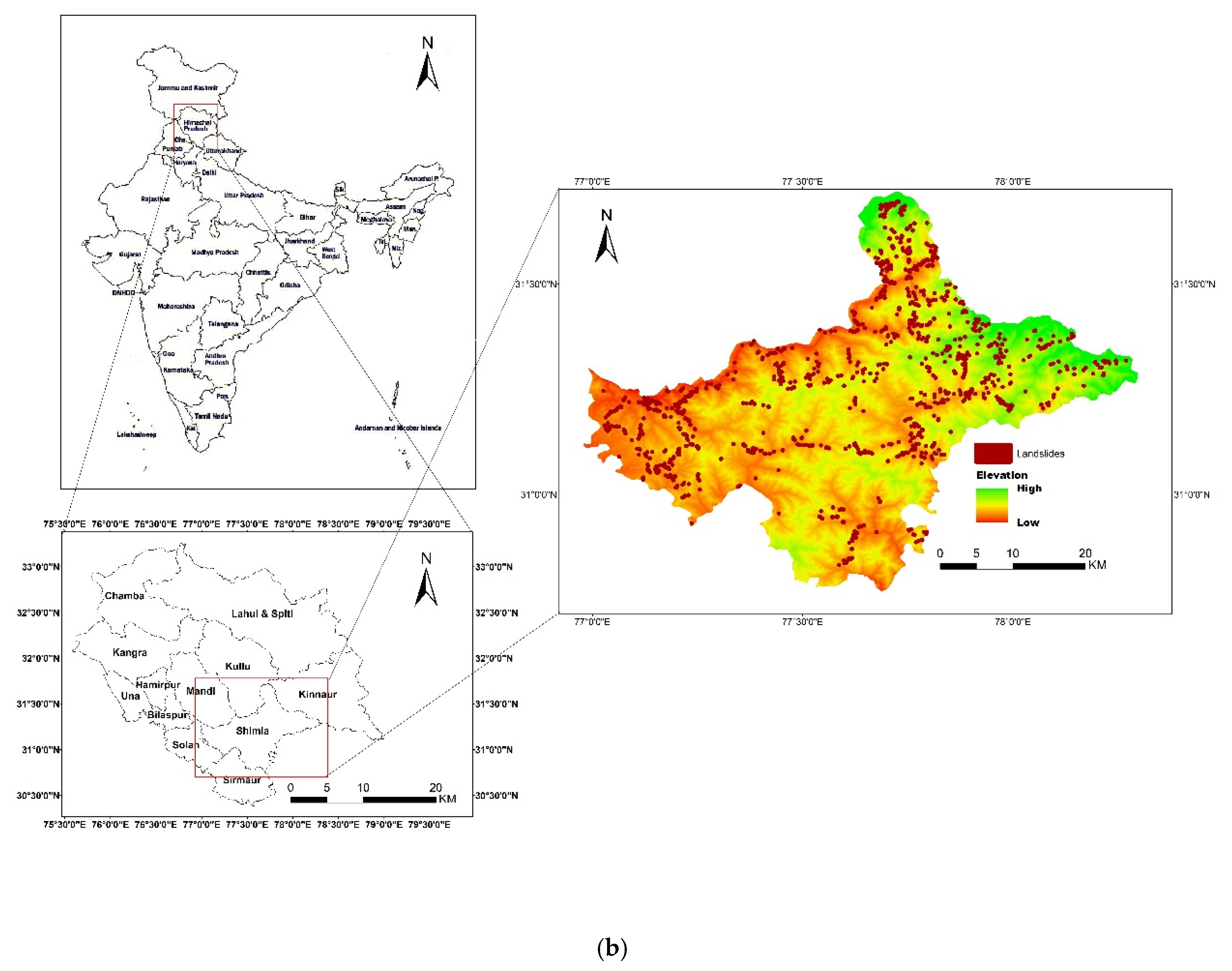
2. Study Area
2.1. Landslide Inventory
2.2. Landslide Conditioning Factors
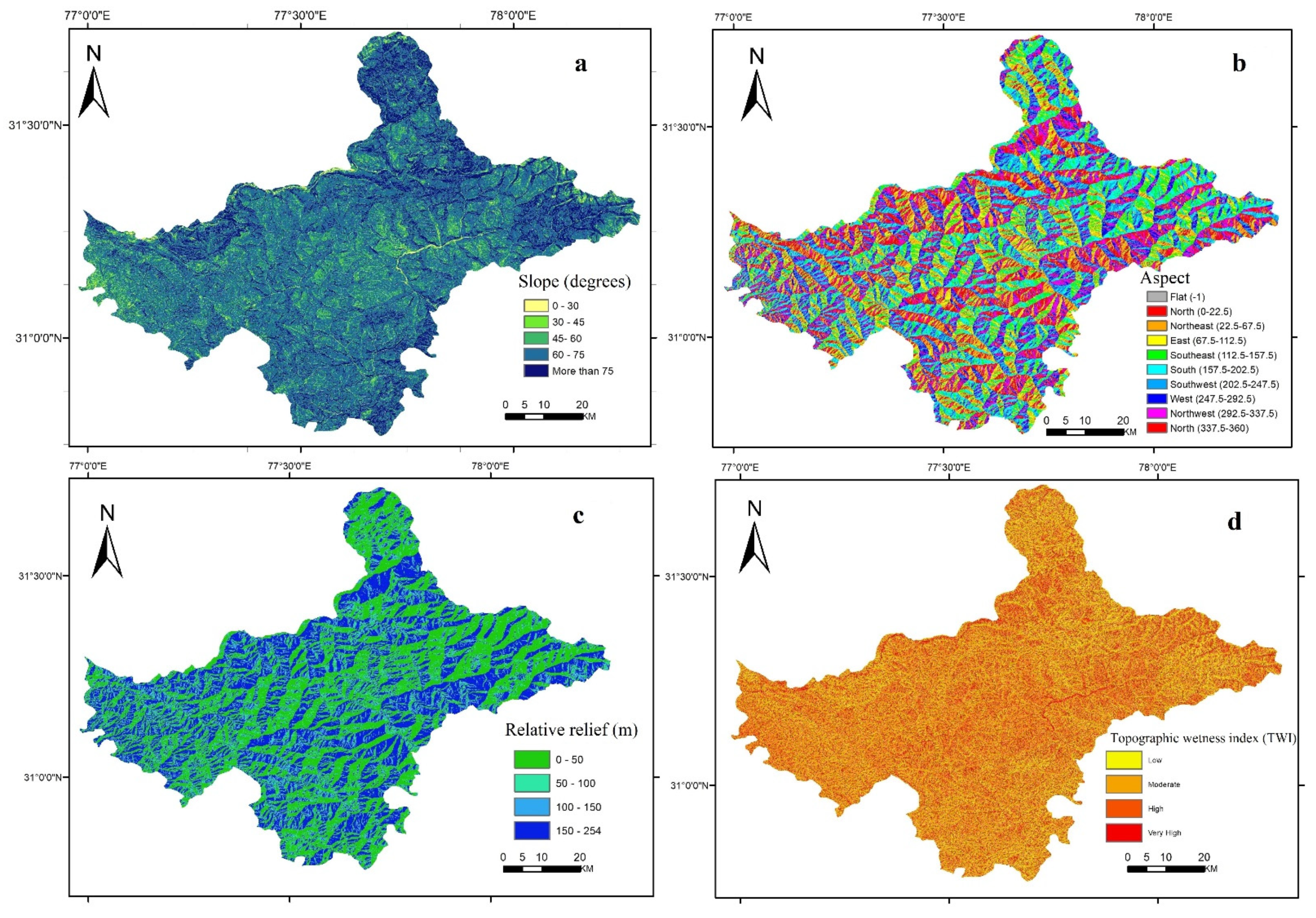
2.2.1. Slope Gradient
2.2.2. Slope Aspect
2.2.3. Relative Relief
2.2.4. Topographic Wetness Index (TWI)
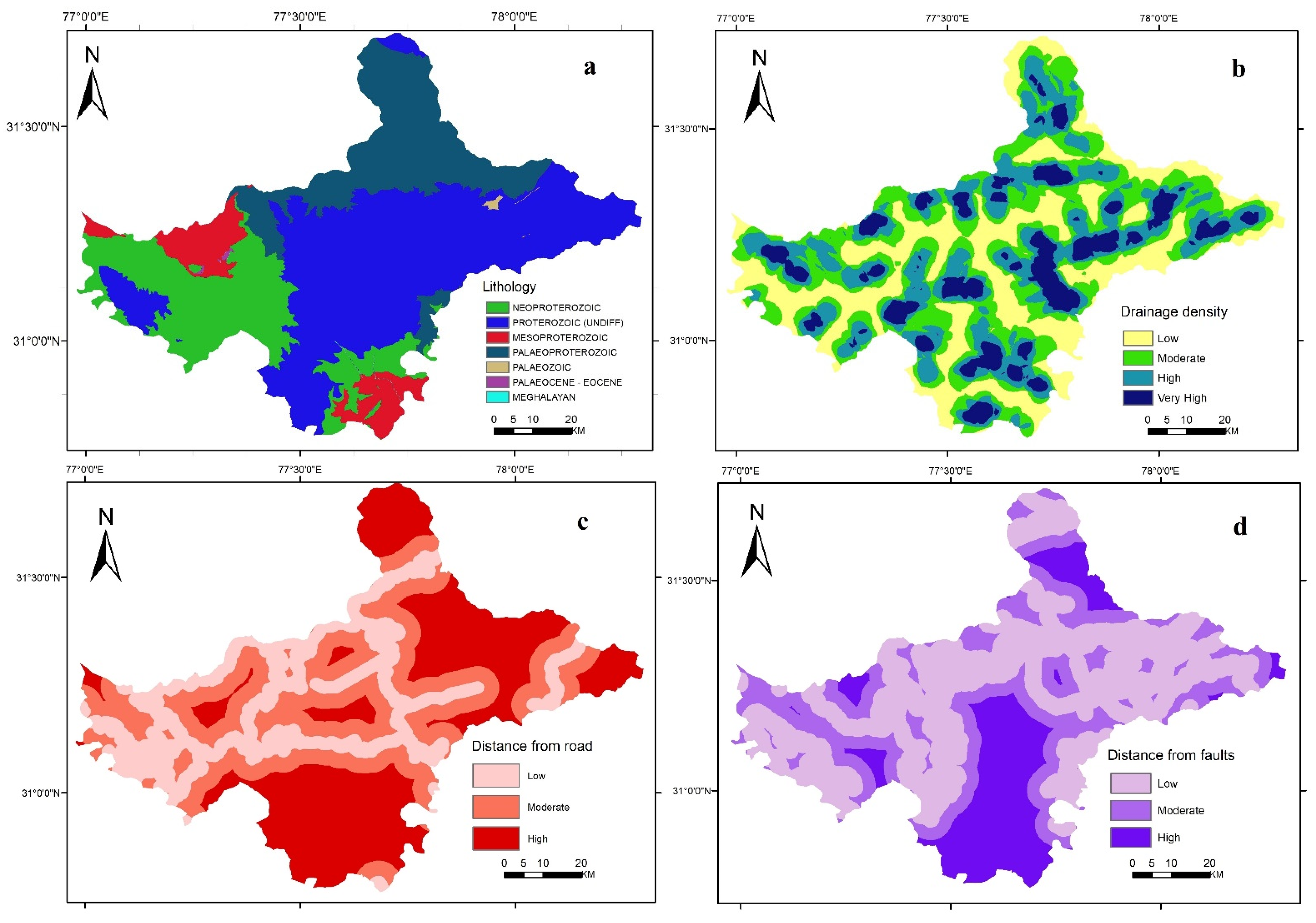
2.2.5. Lithology
2.2.6. Drainage Density
2.2.7. Distance from Roads
2.2.8. Distance from Faults
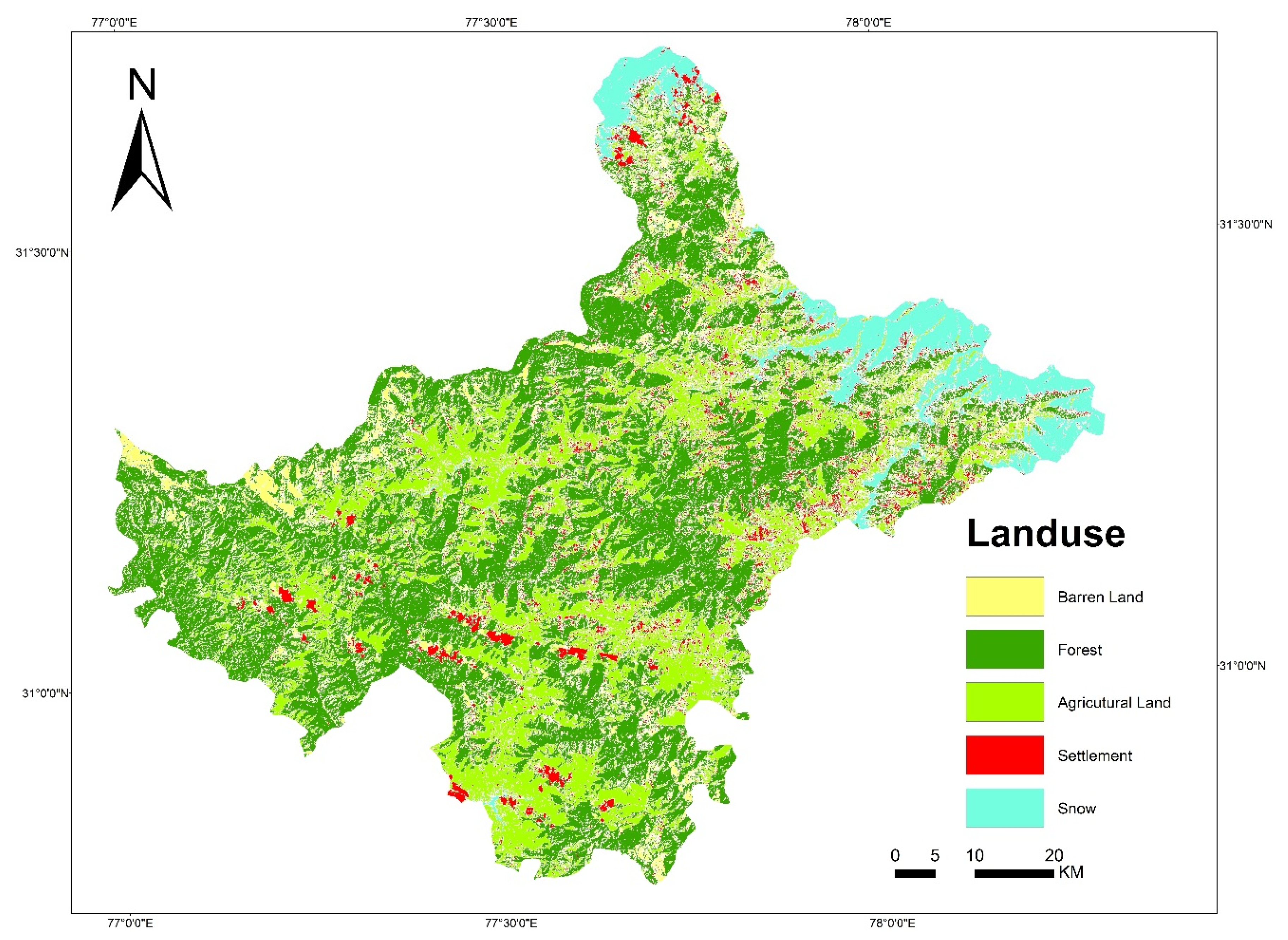
2.2.9. Land Cover
3. Modelling Approach
3.1. Frequency Ratio
3.1.1. Shannon’s Entropy
3.1.2. Analytic Hierarchy Process (AHP)
4. Results and Discussion
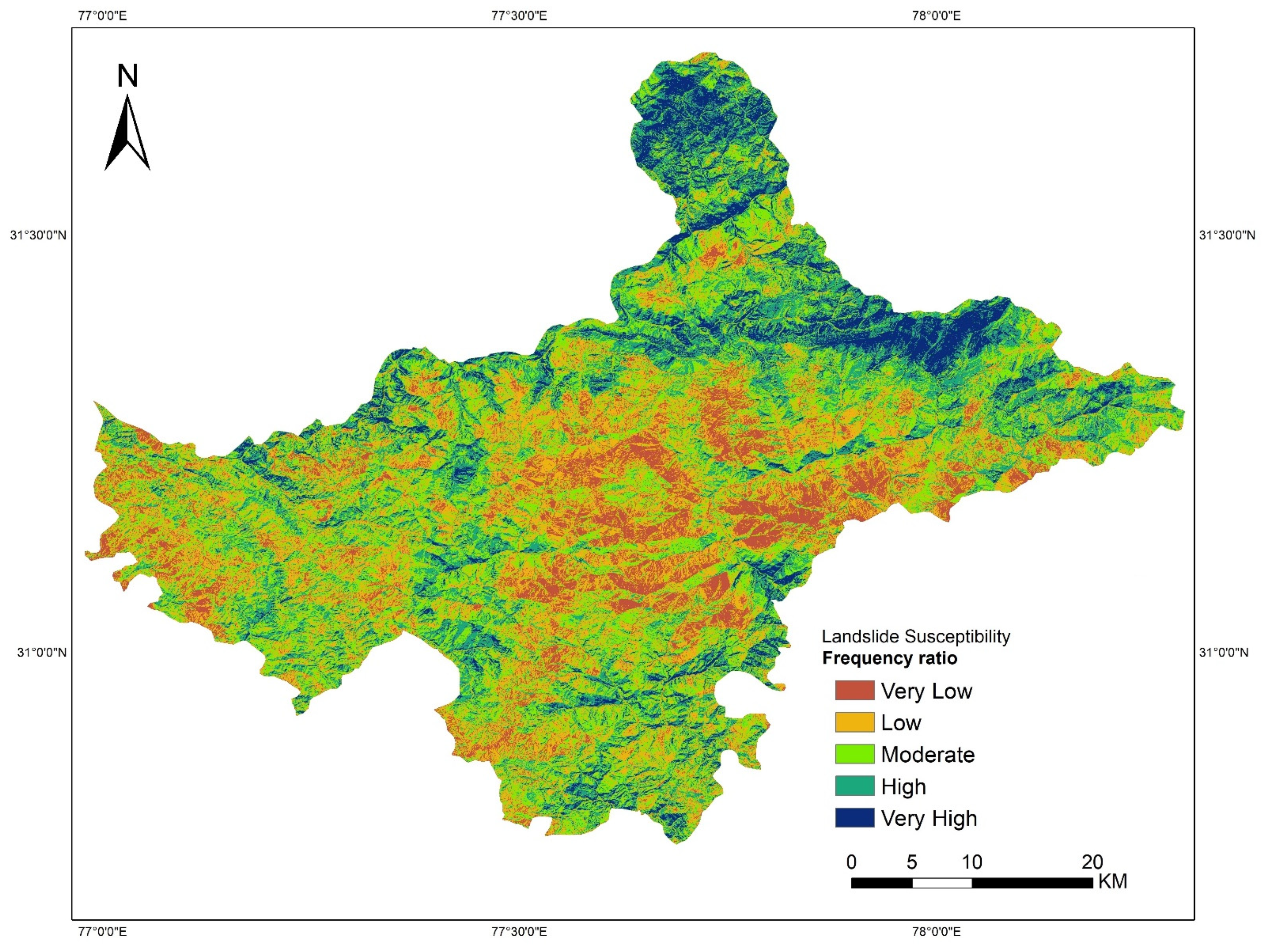
4.1. Frequency Ratio
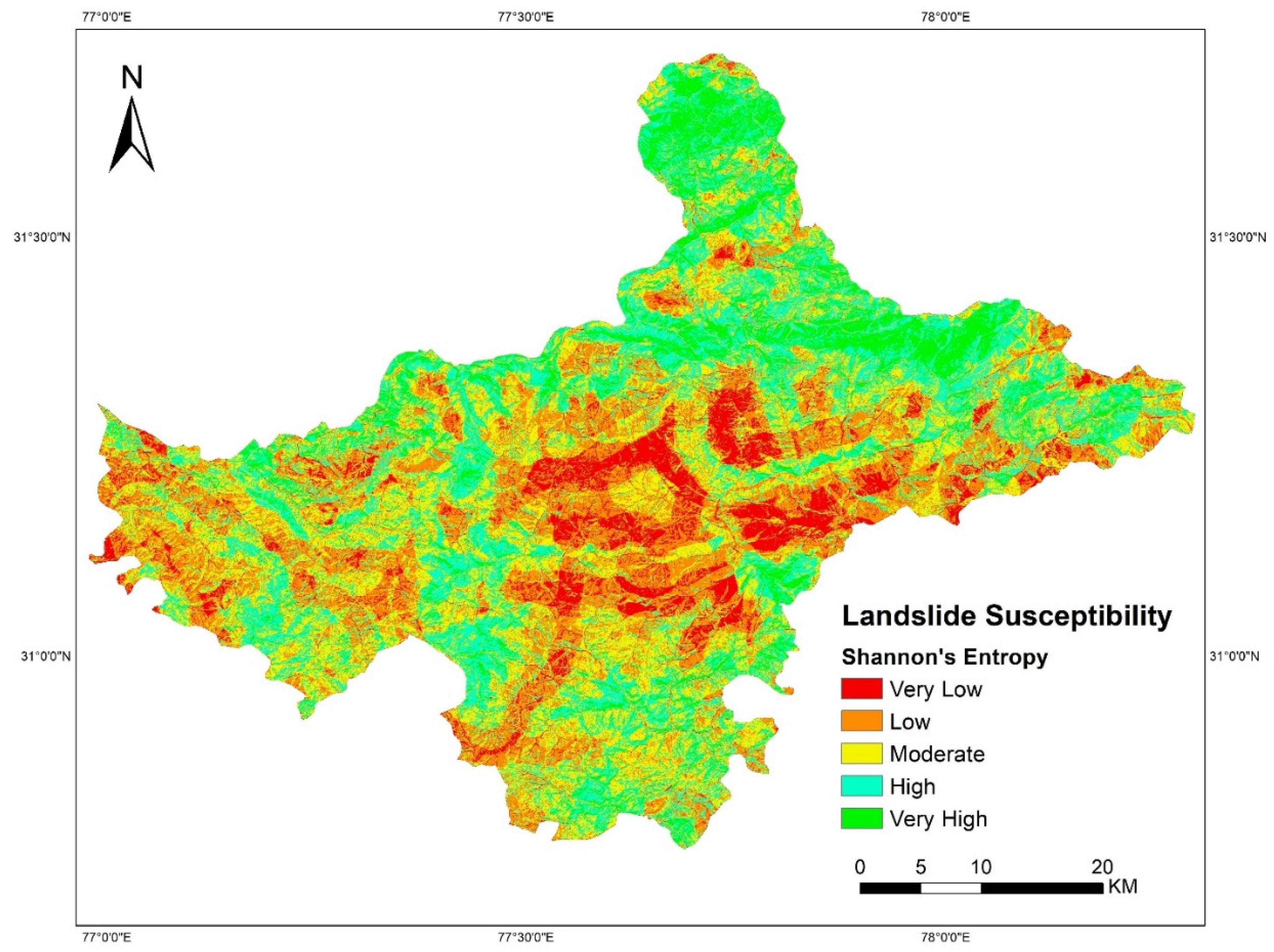
4.2. Shannon’s Entropy Model
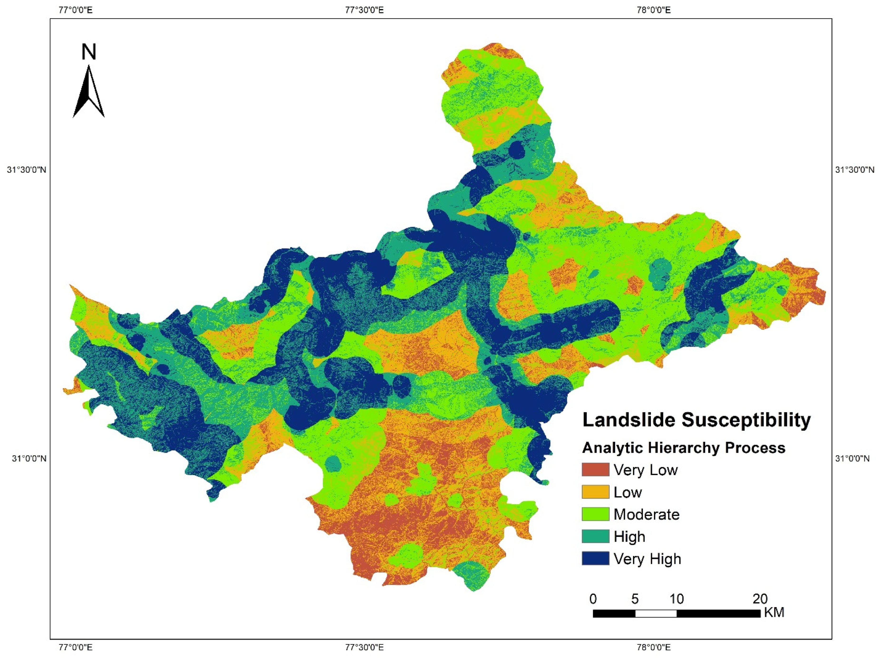
4.3. Analytic Hierarchy Process (AHP) Approach
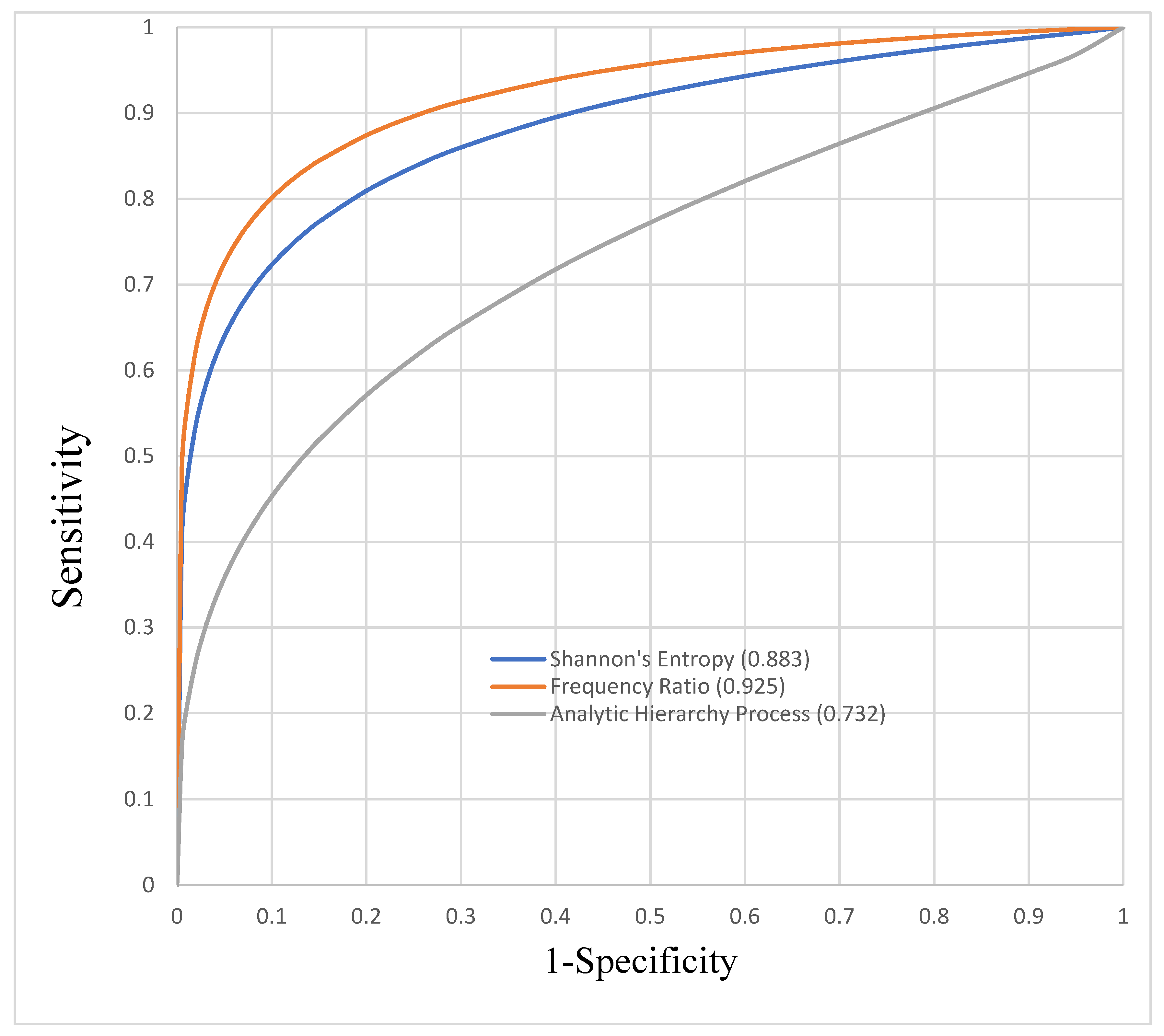
4.4. Validation of Results
5. Conclusions and Future Scope
Author Contributions
Funding
Data Availability Statement
Conflicts of Interest
References
- Aleotti, P.; Chowdhury, R. Landslide hazard assessment: Summary review and new perspectives. Bull. Int. Assoc. Eng. Geol. 1999, 58, 21–44. [Google Scholar] [CrossRef]
- Lee, S. Application and verification of fuzzy algebraic operators to landslide susceptibility mapping. Environ. Earth Sci. 2006, 52, 615–623. [Google Scholar] [CrossRef]
- Xu, C.; Xu, X.; Yu, G. Landslides triggered by slipping-fault-generated earthquake on a plateau: An example of the 14 April 2010, Ms 7.1, Yushu, China earthquake. Landslides 2012, 10, 421–431. [Google Scholar] [CrossRef]
- Mersha, T.; Meten, M. GIS-based landslide susceptibility mapping and assessment using bivariate statistical methods in Simada area, northwestern Ethiopia. Geoenviron. Disasters 2020, 7, 20. [Google Scholar] [CrossRef]
- Khan, H.; Shafique, M.; Khan, M.A.; Bacha, M.A.; Shah, S.U.; Calligaris, C. Landslide susceptibility assessment using Frequency Ratio, a case study of northern Pakistan. Egypt. J. Remote Sens. Space Sci. 2018, 22, 11–24. [Google Scholar] [CrossRef]
- Meten, M.; Bhandary, N.P.; Yatabe, R. GIS-based frequency ratio and logistic regression modelling for landslide susceptibility mapping of Debre Sina area in central Ethiopia. J. Mt. Sci. 2015, 12, 1355–1372. [Google Scholar] [CrossRef]
- Van Westen, C.J.; Rengers, N.; Soeters, R. Use of Geomorphological Information in Indirect Landslide Susceptibility Assessment. Nat. Hazards 2003, 30, 399–419. [Google Scholar] [CrossRef]
- Prasad, A.S.; Pandey, B.W.; Leimgruber, W.; Kunwar, R.M. Mountain hazard susceptibility and livelihood security in the upper catchment area of the river Beas, Kullu Valley, Himachal Pradesh, India. Geoenviron. Disasters 2016, 3, 1. [Google Scholar] [CrossRef] [Green Version]
- Gokceoglu, C.; Aksoy, H. Landslide susceptibility mapping of the slopes in the residual soils of the Mengen region (Turkey) by deterministic stability analyses and image processing techniques. Eng. Geol. 1996, 44, 147–161. [Google Scholar] [CrossRef]
- Lee, S.; Ryu, J.-H.; Won, J.-S.; Park, H.-J. Determination and application of the weights for landslide susceptibility mapping using an artificial neural network. Eng. Geol. 2003, 71, 289–302. [Google Scholar] [CrossRef]
- Yeon, Y.-K.; Han, J.-G.; Ryu, K.H. Landslide susceptibility mapping in Injae, Korea, using a decision tree. Eng. Geol. 2010, 116, 274–283. [Google Scholar] [CrossRef]
- Pourghasemi, H.R.; Mohammady, M.; Pradhan, B. Landslide susceptibility mapping using index of entropy and conditional probability models in GIS: Safarood Basin, Iran. Catena 2012, 97, 71–84. [Google Scholar] [CrossRef]
- Singh, K.; Kumar, V. Hazard assessment of landslide disaster using information value method and analytical hierarchy process in highly tectonic Chamba region in bosom of Himalaya. J. Mt. Sci. 2018, 15, 808–824. [Google Scholar] [CrossRef]
- Gautam, P.; Kubota, T.; Sapkota, L.M.; Shinohara, Y. Landslide susceptibility mapping with GIS in high mountain area of Nepal: A comparison of four methods. Environ. Earth Sci. 2021, 80, 359. [Google Scholar] [CrossRef]
- Hasekioğulları, G.D.; Ercanoglu, M. A new approach to use AHP in landslide susceptibility mapping: A case study at Yenice (Karabuk, NW Turkey). Nat. Hazards 2012, 63, 1157–1179. [Google Scholar] [CrossRef]
- Kayastha, P.; Dhital, M.; De Smedt, F. Application of the analytical hierarchy process (AHP) for landslide susceptibility mapping: A case study from the Tinau watershed, west Nepal. Comput. Geosci. 2013, 52, 398–408. [Google Scholar] [CrossRef]
- El Jazouli, A.; Barakat, A.; Khellouk, R. GIS-multicriteria evaluation using AHP for landslide susceptibility mapping in Oum Er Rbia high basin (Morocco). Geoenviron. Disasters 2019, 6, 3. [Google Scholar] [CrossRef]
- Sujatha, E.R.; Sridhar, V. Mapping debris flow susceptibility using analytical network process in Kodaikkanal Hills, Tamil Nadu (India). J. Earth Syst. Sci. 2017, 126, 116. [Google Scholar] [CrossRef] [Green Version]
- Shahabi, H.; Ahmad, B.B.; Khezri, S. Evaluation and comparison of bivariate and multivariate statistical methods for landslide susceptibility mapping (case study: Zab basin). Arab. J. Geosci. 2012, 6, 3885–3907. [Google Scholar] [CrossRef]
- Kavzoglu, T.; Sahin, E.K.; Colkesen, I. An assessment of multivariate and bivariate approaches in landslide susceptibility mapping: A case study of Duzkoy district. Nat. Hazards 2014, 76, 471–496. [Google Scholar] [CrossRef]
- Ram, P.; Gupta, V.; Devi, M.; Vishwakarma, N. Landslide susceptibility mapping using bivariate statistical method for the hilly township of Mussoorie and its surrounding areas, Uttarakhand Himalaya. J. Earth Syst. Sci. 2020, 129, 167. [Google Scholar] [CrossRef]
- Pradhan, B. Landslide susceptibility mapping of a catchment area using frequency ratio, fuzzy logic and multivariate logistic regression approaches. J. Indian Soc. Remote Sens. 2010, 38, 301–320. [Google Scholar] [CrossRef]
- Sarkar, S.; Roy, A.; Martha, T.R. Landslide susceptibility assessment using Information Value Method in parts of the Darjeeling Himalayas. J. Geol. Soc. India 2013, 82, 351–362. [Google Scholar] [CrossRef]
- Akgun, A.; Erkan, O. Landslide susceptibility mapping by geographical information system-based multivariate statistical and deterministic models: In an artificial reservoir area at Northern Turkey. Arab. J. Geosci. 2016, 9, 165. [Google Scholar] [CrossRef]
- Pradhan, B.; Oh, H.-J.; Buchroithner, M. Weights-of-evidence model applied to landslide susceptibility mapping in a tropical hilly area. Geomat. Nat. Hazards Risk 2010, 1, 199–223. [Google Scholar] [CrossRef]
- Polykretis, C.; Chalkias, C. Comparison and evaluation of landslide susceptibility maps obtained from weight of evidence, logistic regression, and artificial neural network models. Nat. Hazards 2018, 93, 249–274. [Google Scholar] [CrossRef]
- Shano, L.; Raghuvanshi, T.K.; Meten, M. Landslide susceptibility evaluation and hazard zonation techniques—A review. Geoenviron. Disasters 2020, 7, 1–19. [Google Scholar] [CrossRef]
- Mathews, R.P. Ground Information Water Booklet Shimla District, Himachal Pradesh, Ministry of Water Resources, Central Ground Water Board, Government of India. 2013. Available online: http://cgwb.gov.in/District_Profile/HP/Shimla.pdf (accessed on 1 April 2021).
- District Survey Document Shimla. Available online: https://emerginghimachal.hp.gov.in/miningstone/survay_docs/shimla.pdf (accessed on 3 May 2021).
- Guzzetti, F.; Mondini, A.C.; Cardinali, M.; Fiorucci, F.; Santangelo, M.; Chang, K.-T. Landslide inventory maps: New tools for an old problem. Earth Sci. Rev. 2012, 112, 42–66. [Google Scholar] [CrossRef] [Green Version]
- Regmi, A.D.; Yoshida, K.; Pourghasemi, H.R.; DhitaL, M.R.; Pradhan, B. Landslide susceptibility mapping along Bhalubang—Shiwapur area of mid-Western Nepal using frequency ratio and conditional probability models. J. Mt. Sci. 2014, 11, 1266–1285. [Google Scholar] [CrossRef]
- Saleem, N.; Huq, E.; Twumasi, N.Y.D.; Javed, A.; Sajjad, A. Parameters Derived from and/or Used with Digital Elevation Models (DEMs) for Landslide Susceptibility Mapping and Landslide Risk Assessment: A Review. ISPRS Int. J. Geo-Inf. 2019, 8, 545. [Google Scholar] [CrossRef] [Green Version]
- Bahrami, S.; Rahimzadeh, B.; Khaleghi, S. Analyzing the effects of tectonic and lithology on the occurrence of landslide along Zagros ophiolitic suture: A case study of Sarv-Abad, Kurdistan, Iran. Bull. Int. Assoc. Eng. Geol. 2019, 79, 1619–1637. [Google Scholar] [CrossRef]
- Nebeokike, U.C.; Igwe, O.; Egbueri, J.C.; Ifediegwu, S.I. Erodibility characteristics and slope stability analysis of geological units prone to erosion in Udi area, southeast Nigeria. Model. Earth Syst. Environ. 2020, 6, 1061–1074. [Google Scholar] [CrossRef]
- Nepal, N.; Chen, J.; Chen, H.; Wang, X.; Sharma, T.P.P. Assessment of landslide susceptibility along the Araniko Highway in Poiqu/Bhote Koshi/Sun Koshi Watershed, Nepal Himalaya. Prog. Disaster Sci. 2019, 3, 100037. [Google Scholar] [CrossRef]
- Sen, S.; Mitra, S.; Debbarma, C.; De, S.K. Impact of faults on landslide in the Atharamura Hill (along the NH 44), Tripura. Environ. Earth Sci. 2014, 73, 5289–5298. [Google Scholar] [CrossRef]
- Yang, L.; Liu, E. Numerical Analysis of the Effects of Crack Characteristics on the Stress and Deformation of Unsaturated Soil Slopes. Water 2020, 12, 194. [Google Scholar] [CrossRef] [Green Version]
- Demir, G.; Aytekin, M.; Akgun, A. Landslide susceptibility mapping by frequency ratio and logistic regression methods: An example from Niksar–Resadiye (Tokat, Turkey). Arab. J. Geosci. 2014, 8, 1801–1812. [Google Scholar] [CrossRef]
- Park, S.; Choi, C.; Kim, B.; Kim, J. Landslide susceptibility mapping using frequency ratio, analytic hierarchy process, logistic regression, and artificial neural network methods at the Inje area, Korea. Environ. Earth Sci. 2012, 68, 1443–1464. [Google Scholar] [CrossRef]
- Silalahi, F.E.S.; Arifianti, Y.; Hidayat, F. Landslide susceptibility assessment using frequency ratio model in Bogor, West Java, Indonesia. Geosci. Lett. 2019, 6, 10. [Google Scholar] [CrossRef] [Green Version]
- Roodposhti, M.S.; Aryal, J.; Shahabi, H.; Safarrad, T. Fuzzy Shannon Entropy: A Hybrid GIS-Based Landslide Susceptibility Mapping Method. Entropy 2016, 18, 343. [Google Scholar] [CrossRef]
- Sharma, L.P.; Patel, N.; Ghose, M.K.; Debnath, P. Development and application of Shannon’s entropy integrated information value model for landslide susceptibility assessment and zonation in Sikkim Himalayas in India. Nat. Hazards 2014, 75, 1555–1576. [Google Scholar] [CrossRef]
- Saaty, R.W. The analytic hierarchy process—what it is and how it is used. Math. Model. 1987, 9, 161–176. [Google Scholar] [CrossRef] [Green Version]
- Zhu, L.; Huang, J.-F. GIS-based logistic regression method for landslide susceptibility mapping in regional scale. J. Zhejiang Univ. A 2006, 7, 2007–2017. [Google Scholar] [CrossRef]
- Map of India. Available online: https://d-maps.com/ (accessed on 2 January 2021).


| Age | Group Name | Geological Formation | Lithology |
|---|---|---|---|
| Mesoproterozoic | Shali | Tatapani | Pink and grey dolomite, phyllite, shale |
| Neoproterozoic | Shali | Sorgharwari | Pink and grey limestone, sporadic shale |
| Palaeocene-Eocene | Sirmur Dharmshala Group | Subathu | Green carbonaceous shale, limestone, quartzite |
| Palaeoproterozoic | Kulu | Khokhan | Schist and quartzite |
| Palaeozoic | Not available | Not available | Medium to coarse biotite granite |
| Proterozoic (Undiff) | Jutogh | Manal, chor, pabar | White grey quartzite, schist, carbonaceous dolomite, granite, gneiss |
| Conditioning Factor | Classes | No. of Pixels in Class | Percentage in Class (a) | No. of Landslide Pixel in Class | Percentage of Landslide Pixel (b) | FR (b/a) | Pij | Eij | Hij = 1 − Eij | Wj |
|---|---|---|---|---|---|---|---|---|---|---|
| Slope | ||||||||||
| <30 | 107,718.000 | 1.710 | 13.000 | 0.800 | 0.468 | 0.115 | −0.108 | 0.442 | 0.120 | |
| 30–45 | 246,772.000 | 3.900 | 13.000 | 0.800 | 0.205 | 0.050 | −0.065 | |||
| 45–60 | 1,001,205.000 | 15.910 | 91.000 | 5.950 | 0.374 | 0.092 | −0.095 | |||
| 60–75 | 3,779,957.000 | 60.050 | 803.000 | 52.510 | 0.874 | 0.214 | −0.143 | |||
| More than 75 | 1,158,974.000 | 18.410 | 609.000 | 39.830 | 2.163 | 0.530 | −0.146 | |||
| 6,294,626.000 | 1529.000 | 4.085 | −0.558 | |||||||
| Aspect | ||||||||||
| Flat | 105.000 | 0.002 | 0.000 | 0.000 | 0.000 | 0.000 | 0.000 | 0.124 | 0.033 | |
| North | 916,307.000 | 14.560 | 210.000 | 13.730 | 0.943 | 0.116 | −0.108 | |||
| Northeast | 792,179.000 | 12.590 | 156.000 | 10.200 | 0.810 | 0.100 | −0.100 | |||
| East | 627,294.000 | 9.970 | 255.000 | 16.680 | 1.673 | 0.206 | −0.141 | |||
| South East | 804,073.000 | 12.770 | 290.000 | 18.970 | 1.486 | 0.183 | −0.135 | |||
| South | 900,237.000 | 14.310 | 230.000 | 15.040 | 1.051 | 0.129 | −0.115 | |||
| South West | 809,177.000 | 12.860 | 135.000 | 8.830 | 0.687 | 0.084 | −0.091 | |||
| West | 643,538.000 | 10.220 | 150.000 | 9.810 | 0.960 | 0.118 | −0.109 | |||
| North West | 801,716.000 | 12.730 | 103.000 | 6.740 | 0.529 | 0.065 | −0.077 | |||
| 6,294,626.000 | 1529.000 | 100.000 | 8.139 | −0.876 | ||||||
| Relative relief | ||||||||||
| 0−50 | 2,612,642.000 | 41.660 | 804.000 | 52.580 | 1.262 | 0.323 | −0.159 | 0.408 | 0.110 | |
| 50−100 | 691,263.000 | 11.023 | 145.000 | 9.480 | 0.860 | 0.220 | −0.145 | |||
| 100−150 | 710,948.000 | 11.337 | 186.000 | 12.160 | 1.073 | 0.274 | −0.154 | |||
| More than 150 | 2,256,417.000 | 35.980 | 394.000 | 25.770 | 0.716 | 0.183 | −0.135 | |||
| 6,271,270.000 | 1529.000 | 3.911 | −0.592 | |||||||
| TWI | ||||||||||
| Low | 2,810,725.000 | 44.650 | 712.000 | 46.560 | 1.043 | 0.340 | −0.159 | 0.500 | 0.135 | |
| Moderate | 2,473,126.000 | 39.290 | 596.000 | 38.980 | 0.992 | 0.323 | −0.159 | |||
| High | 855,581.000 | 13.590 | 207.000 | 13.540 | 0.996 | 0.325 | −0.159 | |||
| Very High | 155,194.000 | 24.650 | 14.000 | 0.910 | 0.037 | 0.012 | −0.023 | |||
| 6,294,626.000 | 1529.000 | 3.068 | −0.500 | |||||||
| Lithology | ||||||||||
| Neoproterozoic | 1,364,515.000 | 21.680 | 415.000 | 27.150 | 1.252 | 0.408 | −0.159 | 0.401 | 0.109 | |
| Proterozoic (Undiff) | 3,023,399.000 | 48.030 | 415.000 | 27.140 | 0.565 | 0.184 | −0.135 | |||
| Mesoproterozoic | 502,058.000 | 7.970 | 143.000 | 9.350 | 1.173 | 0.382 | −0.160 | |||
| Plaeoproterozoic | 1,384,339.000 | 22.000 | 556.000 | 36.360 | 1.653 | 0.539 | −0.145 | |||
| Palaeozoic | 10,282.000 | 0.160 | 0.000 | 0.000 | 0.000 | 0.000 | ||||
| Palaleocene-eocene | 7564.000 | 0.130 | 0.000 | 0.000 | 0.000 | 0.000 | ||||
| Meghalayan | 2469.000 | 0.030 | 0.000 | 0.000 | 0.000 | 0.000 | ||||
| 6,294,626.000 | 1529.000 | 4.643 | −0.599 | |||||||
| Drainage density | ||||||||||
| 0–15 | 2,309,122.000 | 36.680 | 320.000 | 20.930 | 0.571 | 0.186 | −0.136 | 0.403 | 0.109 | |
| 15–30 | 2,194,591.000 | 34.860 | 628.000 | 41.070 | 1.178 | 0.384 | −0.160 | |||
| 30–45 | 1,441,690.000 | 22.900 | 438.000 | 28.640 | 1.251 | 0.408 | −0.159 | |||
| More than 45 (up to 66) | 349,223.000 | 5.550 | 143.000 | 9.350 | 1.685 | 0.549 | −0.143 | |||
| 6,294,626.000 | 1529.000 | −0.597 | ||||||||
| Distance from road | ||||||||||
| 0–1.5 KM | 1,743,800.000 | 27.700 | 531.000 | 34.720 | 1.253 | 0.409 | −0.159 | 0.547 | 0.148 | |
| 1.5–5.5 km | 2,114,630.000 | 33.590 | 286.000 | 18.700 | 0.557 | 0.181 | −0.134 | |||
| More than 5.5 | 2,436,196.000 | 38.700 | 712.000 | 46.560 | 1.203 | 0.392 | −0.159 | |||
| 6,294,626.000 | 1529.000 | −0.453 | ||||||||
| Distance from faults | ||||||||||
| 0–1.5KM | 2,790,363.000 | 44.330 | 674.000 | 44.080 | 0.994 | 0.324 | −0.159 | 0.587 | 0.159 | |
| 1.5 km–3.0 km | 1,295,638.000 | 58.660 | 298.000 | 19.490 | 0.332 | 0.108 | −0.105 | |||
| more than 3 km | 2,208,625.000 | 35.090 | 557.000 | 26.420 | 0.753 | 0.245 | −0.150 | |||
| 6,294,626.000 | 1529.000 | −0.413 | ||||||||
| Landuse/landcover | ||||||||||
| Snow | 440,046.000 | 6.990 | 220.000 | 14.390 | 2.059 | 0.671 | −0.116 | 0.287 | 0.078 | |
| Settlement | 604,702.000 | 9.610 | 104.000 | 6.800 | 0.708 | 0.231 | −0.147 | |||
| Agricultural Land | 1,800,554.000 | 28.600 | 246.000 | 16.080 | 0.562 | 0.183 | −0.135 | |||
| Forest | 3,148,252.000 | 50.010 | 855.000 | 55.910 | 1.118 | 0.364 | −0.160 | |||
| Barren Land | 301,072.000 | 4.790 | 104.000 | 6.800 | 1.420 | 0.463 | −0.155 | |||
| 6,294,626.000 | 1529.000 | −0.713 | 3.700 |
| Causative Factors | 1 | 2 | 3 | 4 | 5 | 6 | 7 | 8 | 9 | Weightage |
|---|---|---|---|---|---|---|---|---|---|---|
| Slope | 1 | 0.105 | ||||||||
| Aspect | 0.14 | 1 | 0.016 | |||||||
| Relative relief | 0.33 | 4 | 1 | 0.036 | ||||||
| TWI | 2 | 5 | 3 | 1 | 0.081 | |||||
| Lithology | 0.33 | 6 | 3 | 3 | 1 | 0.096 | ||||
| Drainage density | 3 | 7 | 5 | 3 | 3 | 1 | 0.205 | |||
| Distance from road | 2 | 9 | 7 | 5 | 3 | 3 | 1 | 0.28 | ||
| Distance from faults | 3 | 8 | 6 | 4 | 2 | 0.33 | 0.33 | 1 | 0.161 | |
| Landuse | 0.14 | 2 | 0.33 | 0.14 | 0.14 | 0.14 | 0.14 | 0.17 | 1 | 0.02 |
| CR = 0.09 | ||||||||||
| Conditioning Factor | Classes | 1 | 2 | 3 | 4 | 5 | 6 | 7 | 8 | 9 | Weightage (Wi) |
|---|---|---|---|---|---|---|---|---|---|---|---|
| Slope | 0.04 | ||||||||||
| >30 | 1 | 0.054 | |||||||||
| 30–45 | 2 | 1 | 0.102 | ||||||||
| 45–60 | 3 | 3 | 1 | 0.209 | |||||||
| 60–75 | 5 | 5 | 3 | 1 | 0.596 | ||||||
| More than 75 | 9 | 8 | 7 | 5 | 1 | ||||||
| CR = 0.059 | |||||||||||
| Aspect | |||||||||||
| Flat | 1 | 0.023 | |||||||||
| North | 2 | 1 | 0.047 | ||||||||
| Northeast | 7 | 4 | 1 | 0.204 | |||||||
| East | 4 | 2 | 0.33 | 1 | 0.082 | ||||||
| South East | 9 | 8 | 3 | 4 | 1 | 0.362 | |||||
| South | 5 | 3 | 0.5 | 2 | 0.25 | 1 | 0.125 | ||||
| South West | 4 | 2 | 0.25 | 1 | 0.2 | 0.5 | 1 | 0.078 | |||
| West | 3 | 0.5 | 0.25 | 0.5 | 0.14 | 0.33 | 0.5 | 1 | 0.046 | ||
| North West | 2 | 1 | 0.14 | 0.33 | 0.12 | 0.25 | 0.33 | 0.5 | 1 | 0.033 | |
| CR = 0.025 | |||||||||||
| Relative relief | |||||||||||
| 0–50 | 1 | 0.581 | |||||||||
| 50–100 | 0.33 | 1 | 0.255 | ||||||||
| 100–150 | 0.2 | 0.33 | 1 | 0.114 | |||||||
| More than 150 | 0.11 | 0.2 | 0.33 | 1 | 0.05 | ||||||
| CR = 0.028 | |||||||||||
| TWI | |||||||||||
| Low | 1 | 0.565 | |||||||||
| Moderate | 0.33 | 1 | 0.262 | ||||||||
| High | 0.2 | 0.33 | 1 | 0.118 | |||||||
| Very high | 0.14 | 0.2 | 0.33 | 1 | 0.055 | ||||||
| CR = 0.043 | |||||||||||
| Lithology | |||||||||||
| Neoproterozoic | 1 | 0.194 | |||||||||
| Proterozoic (Undiff.) | 0.33 | 1 | 0.098 | ||||||||
| Mesoproterozoic | 0.5 | 4 | 1 | 0.168 | |||||||
| Palaeoproterozoic | 5 | 7 | 3 | 1 | 0.43 | ||||||
| Palaeozoic | 0.2 | 0.33 | 0.33 | 0.2 | 1 | 0.053 | |||||
| Paleocene-eocene | 0.17 | 0.2 | 0.2 | 0.14 | 0.5 | 1 | 0.033 | ||||
| Meghalayan | 0.2 | 0.14 | 0.14 | 0.11 | 0.33 | 0.5 | 1 | 0.024 | |||
| CR = 0.085 | |||||||||||
| Drainage density | |||||||||||
| Low | 1 | 0.046 | |||||||||
| Moderate | 3 | 1 | 0.094 | ||||||||
| High | 5 | 5 | 1 | 0.203 | |||||||
| Very high | 9 | 7 | 5 | 1 | 0.657 | ||||||
| CR = 0.063 | |||||||||||
| Distance from road | |||||||||||
| Low | 1 | 0.751 | |||||||||
| Moderate | 0.2 | 1 | 0.178 | ||||||||
| High | 0.11 | 0.33 | 1 | 0.07 | |||||||
| CR = 0.03 | |||||||||||
| Distance from faults | |||||||||||
| Low | 1 | 0.751 | |||||||||
| Moderate | 0.2 | 1 | 0.178 | ||||||||
| High | 0.11 | 0.33 | 1 | 0.07 | |||||||
| CR = 0.03 | |||||||||||
| Landuse/Landcover | |||||||||||
| Snow | 1 | 0.5 | |||||||||
| Settlement | 0.14 | 1 | 0.046 | ||||||||
| Agricultural land | 0.11 | 0.5 | 1 | 0.034 | |||||||
| Forest | 0.2 | 5 | 5 | 1 | 0.137 | ||||||
| Barren land | 0.33 | 9 | 7 | 3 | 1 | 0.284 | |||||
| CR = 0.072 | |||||||||||
Publisher’s Note: MDPI stays neutral with regard to jurisdictional claims in published maps and institutional affiliations. |
© 2021 by the authors. Licensee MDPI, Basel, Switzerland. This article is an open access article distributed under the terms and conditions of the Creative Commons Attribution (CC BY) license (https://creativecommons.org/licenses/by/4.0/).
Share and Cite
Panchal, S.; Shrivastava, A.K. A Comparative Study of Frequency Ratio, Shannon’s Entropy and Analytic Hierarchy Process (AHP) Models for Landslide Susceptibility Assessment. ISPRS Int. J. Geo-Inf. 2021, 10, 603. https://0-doi-org.brum.beds.ac.uk/10.3390/ijgi10090603
Panchal S, Shrivastava AK. A Comparative Study of Frequency Ratio, Shannon’s Entropy and Analytic Hierarchy Process (AHP) Models for Landslide Susceptibility Assessment. ISPRS International Journal of Geo-Information. 2021; 10(9):603. https://0-doi-org.brum.beds.ac.uk/10.3390/ijgi10090603
Chicago/Turabian StylePanchal, Sandeep, and Amit K. Shrivastava. 2021. "A Comparative Study of Frequency Ratio, Shannon’s Entropy and Analytic Hierarchy Process (AHP) Models for Landslide Susceptibility Assessment" ISPRS International Journal of Geo-Information 10, no. 9: 603. https://0-doi-org.brum.beds.ac.uk/10.3390/ijgi10090603