Autonomous Obstacle Avoidance Algorithm for Unmanned Surface Vehicles Based on an Improved Velocity Obstacle Method

Abstract

Focusing on the collision avoidance problem for Unmanned Surface Vehicles (USVs) in the scenario of multi-vessel encounters, a USV autonomous obstacle avoidance algorithm based on the improved velocity obstacle method is proposed. The algorithm is composed of two parts: a multi-vessel encounter collision detection model and a path re-planning algorithm. The multi-vessel encounter collision detection model draws on the idea of the velocity obstacle method through the integration of characteristics such as the USV dynamic model in the marine environment, the encountering vessel motion model, and the International Regulations for Preventing Collisions at Sea (COLREGS) to obtain the velocity obstacle region in the scenario of USV and multi-vessel encounters. On this basis, two constraint conditions for the motion state space of USV obstacle avoidance behavior and the velocity obstacle region are added to the dynamic window algorithm to complete a USV collision risk assessment and generate a collision avoidance strategy set. The path re-planning algorithm is based on the premise of the minimum resource cost and uses an improved particle swarm algorithm to obtain the optimal USV control strategy in the collision avoidance strategy set and complete USV path re-planning. Simulation results show that the algorithm can enable USVs to safely evade multiple short-range dynamic targets under COLREGS.

1. Introduction

Unmanned Surface Vehicles (USVs) have broad application prospects in marine environmental monitoring, marine rights and interests maintenance, and military fields and have become a research hotspot in the field of marine intelligent equipment [1,2,3,4]. A safe and reliable path planning method is a prerequisite and allows a USV to perform various complex water surface tasks [5,6,7,8]. However, USVs are affected by many factors, such as the complex marine environment, the dynamic characteristics of USVs, and the performance of the ship-borne detection equipment, which all increase the risk of collisions with other vessels during USV high-speed navigation [9,10,11,12]. Therefore, it is difficult for USV path planning technology to complete collision detection and path re-planning quickly and accurately with less control cost in the complex marine environment.

At present, the algorithms applied for USV autonomous obstacle avoidance include the artificial potential field method, the vector field histogram method, the Set-Based Guidance (SBG) method, the dynamic window method, and the velocity obstacle (VO) method [13,14,15]. Among them, VO has the characteristics of fast response; high real-time performance; strong robustness; and simple and easy realization in the obstacle avoidance problem of intelligent agents, which is widely used for the autonomous obstacle avoidance of agents [16,17]. Fiorini et al. first proposed a VO theoretical model based on the concept of a collision cone. The idea is to construct the velocity obstacle region according to the position information and motion characteristics of the agent and the obstacle and select the feasible velocity vector according to the region involved to complete the avoidance of static or dynamic threats [18]. Based on this, scholars have improved the VO algorithm for different application scenarios. Improved algorithms include the Reciprocal Velocity Obstacle (RVO) [19], Hybrid Reciprocal Velocity Obstacle (HRVO) [20], Probabilistic Reciprocal Velocity Obstacle (PVO) [21], and Generalized Velocity Obstacle (GVO) methods, which consider the rigid motion characteristics of the controlled object [22]. The authors of [23] obtain the collision avoidance priority by calculating the collision threat level of multiple obstacle targets, which improves the accuracy of the collision avoidance strategy of the VO algorithm when avoiding multiple obstacle targets. The authors of [24] introduce the International Regulations for Preventing Collisions at Sea (COLREGS) based on the VO algorithm to ensure that the path of dynamic planning complies with the relevant regulations of COLREGS, but the algorithm does not discuss the generation of a collision avoidance strategy in the scenario of multi-vessel encounters. The authors of [25] use the Monte Carlo method to set ship navigation safety rules in a distributed form based on constructing the probabilistic velocity obstacle region; USV can determine the timing and priority of triggering a collision avoidance strategy according to this rule. However, this method does not consider COLREGS constraint conditions and the dynamic characteristics of USVs in the marine environment, and it is difficult to apply it in actual scenarios. The authors of [26] added the two constraints of agent velocity state space and velocity obstacle region to the dynamic window algorithm to ensure the enforceability of the collision avoidance strategy. The authors of [27] analyze and evaluates the influence of marine environmental disturbances on static obstacles and dynamic ships, and constructs a safe distance constraint model to generate the USV trajectory to improve the safety of path planning. The authors of [28] draw on the idea of the velocity obstacle method and integrate the characteristics of the USV dynamics model, the encountering vessel motion model, COLREGS, etc, construct a USV local trajectory planner to generate real-time trajectories that meet the physical motion characteristics of USV for the USV control system. However, this method does not consider the minimum resource cost between the collision avoidance strategy and the return original path. In summary, in the process of model construction the improved VO method ignores or simplifies COLREGS, the dynamic characteristics of USV in the marine environment, and the motion characteristics of the encountering vessel. Additionally, the minimum resource cost of the USV collision avoidance strategy is not fully considered, which makes it difficult for USVs to complete the autonomous obstacle avoidance task at the minimum cost during high-speed navigation.

Focusing on the above problems, this paper proposes a USV autonomous obstacle avoidance algorithm based on the improved VO method. The algorithm constructs a multi-vessel encounter collision detection model based on constraint models such as USV dynamic characteristics, the encountering vessel motion characteristics, and COLREGS, thereby generating the velocity obstacle region and the USV executable collision avoidance strategy set. On this basis, the degree of collision threat of the encountering vessel is calculated, which provides a basis for the USV to choose the time at which to start the collision avoidance strategy. At the same time, the path re-planning cost function is established on the premise of the minimum resource cost, and the improved particle swarm algorithm is used to speed up the solving speed of the model and, finally, generate a re-planning path conforming to the characteristics of the USV dynamics.

The rest of the paper is organized as follows. Section 2 introduces the problem description and summarizes three sub-problems that need to be solved in the autonomous obstacle avoidance of USVs. Section 3 establishes the USV autonomous obstacle avoidance model based on the improved VO algorithm. Section 4 solves the autonomous obstacle avoidance model of USV based on the improved particle swarm optimization algorithm. Simulation results are shown and analyzed in Section 5. Section 6 concludes this work.

2. Problem Description

USV must have the ability of autonomous obstacle avoidance during multi-vessel encounters when performing channel mapping, ship supervision, and forensics tasks on the sea surface. The USV autonomous obstacle avoidance process can be described as follows: First of all, the USV uses shipborne detection sensors to perceive surrounding vessels—that is, to obtain the position, velocity, water surface contour, and other information of the encountering vessel in real time through its Automatic Identification System (AIS), visual system, laser, or millimeter-wave radar platform shipborne sensing equipment. Secondly, under the constraints of its dynamic characteristics and COLREGS, the USV completes collision detection and a collision threat level assessment according to the physical characteristics of the marine environment, its motion state, and the encountering vessel motion state, generating a collision avoidance strategy set. Then, according to the minimization principle of specific cost (such as control cost, energy consumption cost, etc.), the optimal collision avoidance strategy is obtained and control commands are generated to complete the autonomous obstacle avoidance in the scenario of multi-vessel encounters. Figure 1 shows the autonomous obstacle avoidance process of USV in the scenario of multi-vessel encounters.

USV is an underdrive, large-inertia, and strong time-delay system, and its motion state will be limited by its structure and characteristic parameters. This requires the planned path to satisfy the physical motion characteristics of USV. At the same time, affected by the physical environment characteristics of the ocean and its detection load performance, it is difficult for the USV to complete the detection of multiple vessels remotely, which requires the USV to re-plan efficiently. In addition, to ensure the safety of operations and navigation at sea, this requires the obstacle avoidance measures taken to comply with the provisions of COLREGS when the USV encounters other vessels. Based on this, this paper fully considers the above-mentioned influencing factors; constructs a multi-vessel encounter autonomous obstacle avoidance model of USV under the constraints of the USV dynamic characteristics, the encountering vessel motion characteristics, and COLREGS; and realizes the autonomous and efficient obstacle avoidance of USV. Combined with the principle block diagram of USV autonomous obstacle avoidance shown in Figure 1, this paper decomposes the process of USV autonomous obstacle avoidance into the following three sub-problems:

• Construction of a USV motion model.

The USV mathematical model is the core of the ship motion and control. Establishing an accurate motion model is the prerequisite and basic guarantee for studying the autonomous obstacle avoidance of USVs. As a USV is sailing, its motion performance is greatly affected by the disturbance of the complex external environment, which is mainly reflected in the sea breeze, ocean waves, and ocean currents. Therefore, the construction of the USV motion model needs to fully consider the influence of wind, wave, current, and other external marine environmental disturbances on its motion. Under this constraint, an accurate USV motion model is constructed to determine its system state to ensure the effectiveness of the USV obstacle avoidance behavior.

2.

Efficient characterization of velocity obstacle region.

The operating environment of the USV is highly dynamic and uncertain. When its shipborne sensing equipment detects vessels that pose a threat to USV, timely and effective obstacle avoidance measures need to be taken to ensure the safety of USV navigation. The USV needs to strictly abide by the relevant regulations of COLREGS when operating at sea, and its obstacle avoidance behavior is affected by its motion model and the encountering vessel motion characteristics. Therefore, the construction of the multi-vessel encounter collision detection model needs to comprehensively consider the constraints of the above factors. The model must draw on the idea of VO through the integration of characteristics such as the USV dynamic model in the marine environment, the encountering vessel motion model, and COLREGS to obtain the velocity obstacle region in the scenario of USV and multi-vessel encounters. Based on this, two constraint conditions for the motion state space of USV obstacle avoidance behavior and the velocity obstacle region are added to the dynamic window algorithm to provide a guarantee for USV to generate a collision avoidance strategy set that is executable by the control system; on this basis, the collision threat degree of the encountering vessel is calculated, which provides a decision basis for the USV to choose the time at which to start the collision avoidance strategy.

3.

Construction of an autonomous obstacle avoidance model.

In the process of performing autonomous obstacle avoidance tasks, the USV needs to consider the minimum resource cost between a collision avoidance strategy and returning to the original path while re-planning the path so that USV can efficiently complete the autonomous obstacle avoidance task with the minimum resource cost. Therefore, the construction of the autonomous obstacle avoidance model needs to fully consider the adaptability of the model to the application environment and the application object; establish the path re-planning cost function on the premise of obtaining the minimum resource cost; and use the improved particle swarm algorithm to speed up the solving speed of the model, produce the optimal collision avoidance navigation strategy, and complete USV path re-planning.

3. Autonomous Obstacle Avoidance Model of USV Based on Improved VO

3.1. USV Motion Model in Marine Environment

To fully consider the influence of the marine environment on USV movement, the modeling idea of the mathematical model group of ships (MMG model) is adopted to convert the influence of external disturbances such as wind, wave, and current into the force and torque acting on the USV to construct a motion model of the USV. Assuming that the mass distribution of the USV is uniform, the center of buoyancy coincides with the center of gravity and only the horizontal plane motion of USV is considered—that is, only the surge, sway, and yaw motion. The motion equation of USV can be expressed as:

$$\{\begin{array}{l}\dot{\mathit{\eta }}=J(\mathit{\eta })\mathit{\nu }\\ \left[\begin{array}{cc}\begin{array}{l}I\\ 0\end{array}& \begin{array}{l}0\\ M\end{array}\end{array}\right]\dot{\mathit{X}}=\left[\begin{array}{c}J(\mathit{\eta })\mathit{\nu }\\ -\mathit{C}(\mathit{\nu })\mathit{\nu }-\mathit{D}(\mathit{\nu })\mathit{\nu }\end{array}\right]+\mathit{Q}\left({\tau }_{RB}+{\tau }_{ED}\right)\end{array}$$

(1)

where $\mathit{\eta }={[x,y,\mathit{\psi }]}^{\mathrm{T}}$, respectively, represent the longitudinal displacement, transverse displacement, and yaw angle of the USV in the inertial coordinate system; $\mathit{\nu }={[u,v,r]}^{\mathrm{T}}$, respectively, represent the longitudinal velocity, transverse velocity, and yaw angular velocity of USV in the hull coordinate system; $M$, $C(\mathit{\nu })$, and $D(\mathit{\nu })$ are the inertia matrix, Coriolis-centripetal matrix, damping matrix, and rotation matrix, respectively; $X={[{\mathit{\eta }}^{\mathrm{T}},{\mathit{\nu }}^{\mathrm{T}}]}^{\mathrm{T}}$ represents the system state of USV; ${\tau }_{RB}$ and ${\tau }_{ED}$ represent the force generated by the USV propulsion system and the marine environmental disturbance, respectively; and $Q=\left[\begin{array}{ccc}\begin{array}{cc}\begin{array}{l}0\\ 0\\ 0\end{array}& \begin{array}{cc}\begin{array}{cc}\begin{array}{l}0\\ 0\\ 0\end{array}& \begin{array}{l}0\\ 0\\ 0\end{array}\end{array}& \begin{array}{l}1\\ 1\\ 1\end{array}\end{array}\end{array}& \begin{array}{l}1\\ 1\\ 1\end{array}& \begin{array}{l}1\\ 1\\ 1\end{array}\end{array}\right]$ represents the coefficient matrix used to calculate the thrust and disturbing force in the MMG model.

If the PD controller is used, ${\tau }_{RB}$ expression is shown in Equation (2):

$${\tau }_{RB}=k_p\left(\mathit{u}-\mathit{V}\mathit{X}\right)-k_d\mathit{V}\dot{\mathit{X}}$$

(2)

where $V=\left[\begin{array}{ccc}\begin{array}{cc}\begin{array}{l}0\\ 0\\ 0\end{array}& \begin{array}{cc}\begin{array}{cc}\begin{array}{l}0\\ 0\\ 0\end{array}& \begin{array}{l}0\\ 0\\ 1\end{array}\end{array}& \begin{array}{l}1\\ 0\\ 0\end{array}\end{array}\end{array}& \begin{array}{l}0\\ 1\\ 0\end{array}& \begin{array}{l}0\\ 0\\ 0\end{array}\end{array}\right]$ is the observation matrix and $u$ represents the control input of USV. This paper uses a VO model to avoid obstacles, and for the VO model, $u=\mathit{\nu }={[u,v,r]}^{\mathrm{T}}$.

${\mathit{\tau }}_{ED}$ represents the disturbance effect of the marine environment on USV, and its expression is shown in Equation (3):

$${\tau }_{ED}={\tau }_{wind}+{\tau }_{wave}+{\tau }_{current}$$

(3)

where ${\tau }_{wind}$, ${\tau }_{wave}$, and ${\tau }_{current}$ represent the interference force generated by the wind, waves, and ocean current, respectively. Expressions for these are shown in Equations (4)–(6).

$${\mathit{\tau }}_{wind}=\frac{1}{2}{\rho }_a{V}_w^2\left[\begin{array}{c}{C}_X(\gamma )A_{Fw}\\ C_Y(\gamma )A_{Lw}\\ C_N(\gamma )A_{Lw}L\end{array}\right]$$

(4)

where ${\rho }_a$ represents air density; $V_w$ represents the sea wind speed acting on the USV; $A_{Fw}$ and $A_{Lw}$ represent the area of the USV affected by the sea breeze in the positive and side directions, respectively; $L$ represents the total length of the USV hull; $C_X(\gamma )$, $C_Y(\gamma )$, and $C_N(\gamma )$ are the coefficients of air resistance, which are generally obtained by a ship model test; and $\gamma$ represents the wind direction angle encountered by the USV—namely, the angle between the wind direction and the head and tail connection of the hull.

$${\mathit{\tau }}_{wave}=\left[\begin{array}{l}{\displaystyle \sum _{i=1}^N\rho gBLT\cos (\phi )s_i}(t)\\ {\displaystyle \sum _{i=1}^N-\rho gBLT\sin (\phi )s_i}(t)\\ {\displaystyle \sum _{i=1}^N\frac{1}{24}\rho gBL(L^2-B^2)\sin (2\phi )s_i^2}(t)\end{array}\right]$$

(5)

where $\rho$ represents the density of seawater; $g$ is gravity acceleration; $B$ represents the hull width of the USV; $L$ represents the total length of the USV hull; $T$ means eating water; $\phi$ represents the encounter angle between waves and boats; and $s_i(t)$ represents the spectrum of waves.

$${\tau }_{current}=\frac{1}{2}\rho V_c^2\left[\begin{array}{c}{A}_{FC}{c}_X(\alpha )\\ A_{LC}{c}_Y(\alpha )\\ A_{LC}{c}_N(\alpha )L\end{array}\right]$$

(6)

where $\rho$ represents the density of seawater; $V_c$ represents the speed of the ocean current, $A_{FC}$ and $A_{LC}$ represent the area to the front and sides of the underwater part that are affected by the waves; $c_X(\alpha )$, $c_Y(\alpha )$, and $c_N(\alpha )$ represent the calculation coefficients of the force and moment of the ocean current, which are generally obtained by ship model experiments; and $\alpha$ is the angle of encounter between the ocean current and the hull; $L$ represents the total length of the USV hull.

By substituting Equations (2) and (3) into Equation (1), we can obtain the nonlinear ordinary differential equation of the system state, as shown in Equation (7).

$$\begin{array}{cc}\dot{\mathit{X}}& ={\left[\left[\begin{array}{cc}\begin{array}{l}I\\ 0\end{array}& \begin{array}{l}0\\ M\end{array}\end{array}\right]+Q{k}_{d}V\right]}^{-1}\left[\begin{array}{c}J(\mathit{\eta })u\\ -C(u)u-D(u)u\end{array}\right]+{\left[\left[\begin{array}{cc}\begin{array}{l}I\\ 0\end{array}& \begin{array}{l}0\\ M\end{array}\end{array}\right]+Q{k}_{d}V\right]}^{-1}Q{k}_p\left(u-VX\right)\\ & +{\left[\left[\begin{array}{cc}\begin{array}{l}I\\ 0\end{array}& \begin{array}{l}0\\ M\end{array}\end{array}\right]+Q{k}_{d}V\right]}^{-1}Q{\mathit{\tau }}_{ED}\hfill \\ & =f\left(X,u\right)\hfill \end{array}$$

(7)

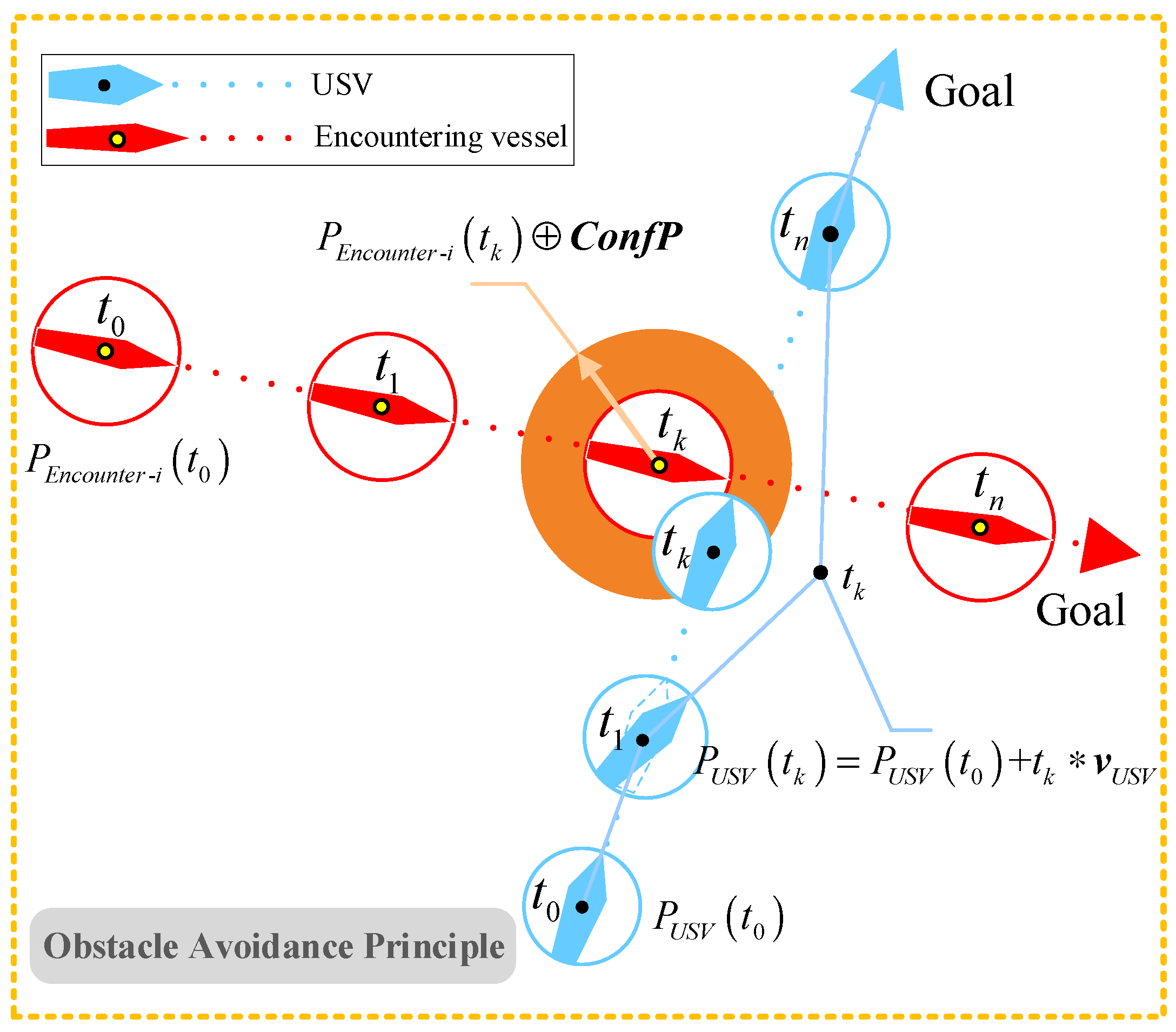
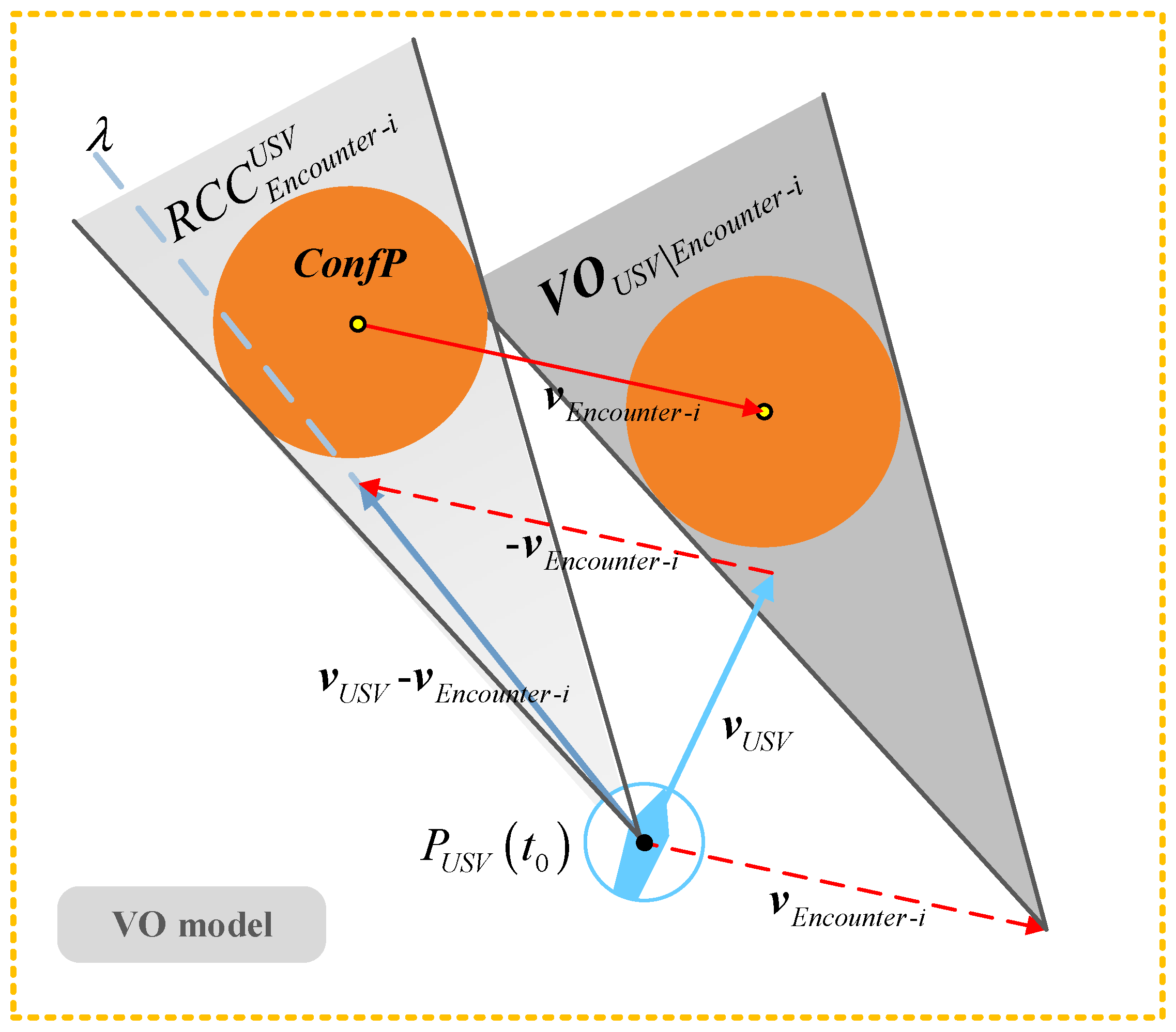
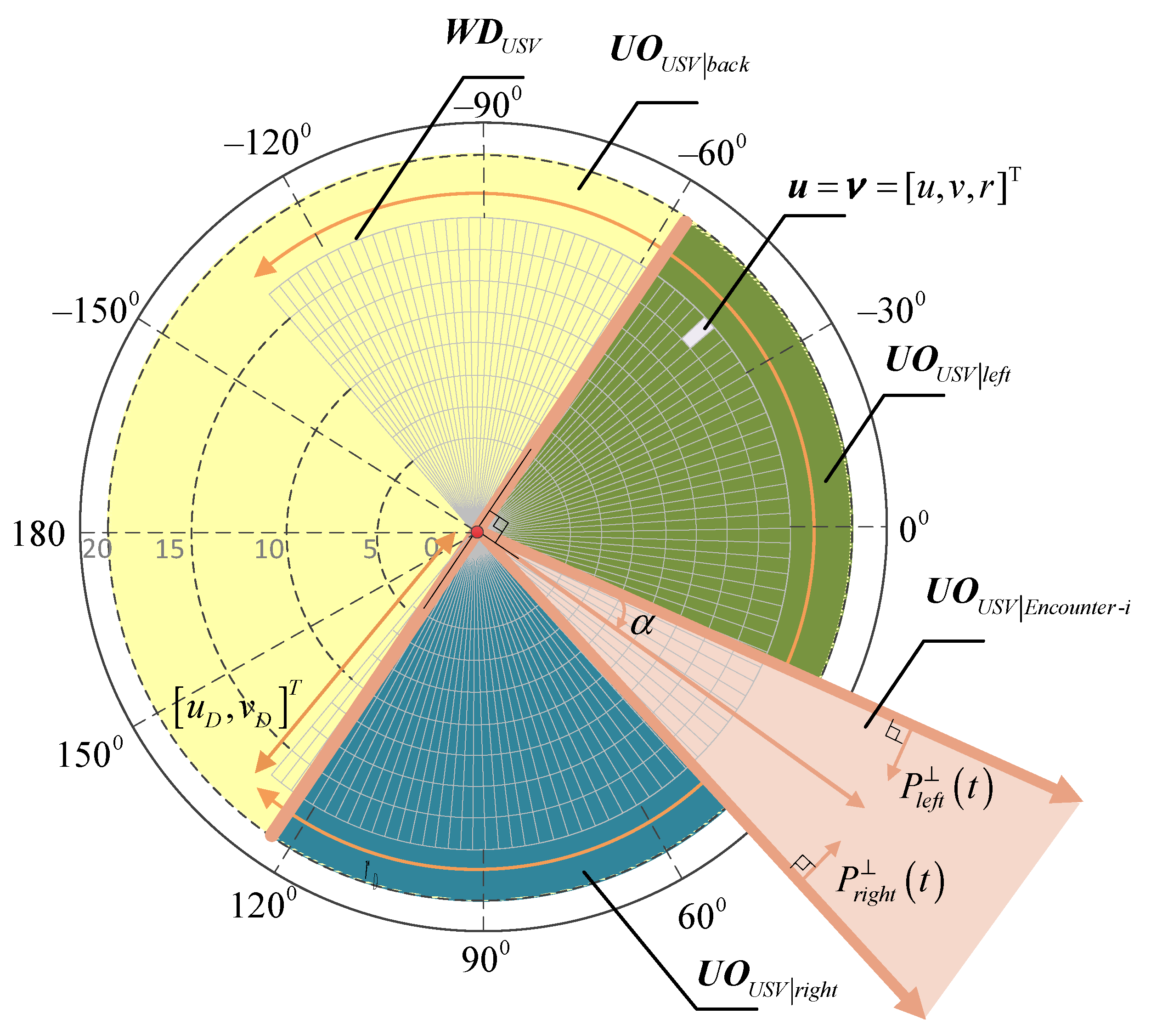
3.2. Efficient Characterization of Velocity Obstacle Region

A scenario of a USV encounter with other vessels during the voyage is shown in Figure 2. In Figure 2, the blue ship represents the USV and the red ship represents the encountering vessel. It can be seen from Figure 2 that when the position of the USV is within the safe distance of the encountering vessel, the two ships will collide. The condition for the USV to collide with the encountering vessels can be expressed as:

$$\{\begin{array}{l}{P}_{USV}(t_k)\in P_{Encounter-i}(t_k)\oplus ConfP\\ ConfP=\left\{\Vert P_{USV}(t_k)-P_{Encounter-i}\left(t_k\right)\Vert \le R\right\}\hspace{0.17em}\hspace{0.17em},R=R_{USV}+R_{Encounter-i}\end{array}$$

(8)

where $P_{USV}(t_k)=[x_{USV}(t_k),y_{USV}(t_k)]$ and $P_{Encounter-i}(t_k)=[x_{Encounter-i}(t_k),y_{Encounter-i}(t_k)]$ are the positions of the USV and the encountering vessel at the time $t_k$, respectively; $\oplus$ is the Minkowski vector sum operation; and $\Vert \cdot \Vert$ represents the Euclidean distance; $ConfP$ represents a group of positions leading to conflicts between two ships, whose size and shape depend on the ship domain characteristics of the USV and the encountering vessel. For the convenience of expression and calculation, this paper expresses the ship domain characteristics of the USV and the encountering vessel as a circle with the length of the ship as its diameter, where the radius of the circle for each is $R_{USV}$ and $R_{Encounter-i}$, respectively. The sum of the radius $R$ is the radius of $ConfP$; the center of $ConfP$ is the center of the encountering vessel; and $P_{Encounter-i}(\cdot )\oplus ConfP$ represents all possible location areas where two ships can collide at a certain time.

Assuming that, from time $t_{k-1}$ to time $t_k$, the USV and the encountering vessel move in a straight line at a uniform speed, then the positions of the USV and the encountering vessel at the time $t_k$ are shown in Equation (9):

$$\{\begin{array}{l}{P}_{USV}(t_k)=P_{USV}(t_{k-1})+(t_k-t_{k-1})\cdot v_{USV}(t_k,t_{k-1})\\ P_{Encounter-i}(t_k)=P_{Encounter-i}(t_{k-1})+(t_k-t_{k-1})\cdot v_{Encounter-i}(t_k,t_{k-1})\end{array}$$

(9)

where $P_{USV}(t_{k-1})$ and $P_{Encounter-i}(t_{k-1})$ represent the positions of the USV and the encountering vessel at the time $t_{k-1}$, respectively. $v_{USV}(t_k,t_{k-1})$ and $v_{Encounter-i}(t_k,t_{k-1})$ represent the velocity vectors of the USV and the encountering vessel in the period $[t_k,t_{k-1})$, respectively. According to Equation (8), if $P_{USV}(t_k)$ includes $P_{Encounter-i}\left(t_k\right)\oplus ConfP$, USV will collide with the encountering vessel at the time $t_k$. Therefore, to achieve the purpose of avoiding vessels, the USV can adjust $v_{USV}(t_k,t_{k-1})$ to make $t_k$ time $P_{USV}(t_k)$ outside $P_{Encounter-i}\left(t_k\right)\oplus ConfP$.

Characterize of Velocity Obstacle Region Based on VO

The VO algorithm is a widely used USV autonomous dynamic obstacle avoidance algorithm. It uses the position information and motion characteristics of the USV and the encountering vessel to construct the velocity obstacle region; on this basis, it selects a feasible velocity vector to complete the rapid avoidance of static or dynamic threats and has the characteristics of fast response and simple realization. The corresponding geometric model is shown in Figure 3.

Figure 3 shows that the velocity obstacle region characterized by the VO model is the conical area surrounded by taking $P_{USV}(t_{k-1})$ as the starting point to make two tangents $ConfP$. This area is the velocity obstacle region between the encountering vessel and the USV, denoted as $RC{C}_{Encounter-i}^{USV}$.

Let $\lambda =\left\{P_{USV}(t_{k-1})+(t_k-t_{k-1})\cdot \left(v_{USV}(t_k,t_{k-1})-v_{Encounter-i}(t_k,t_{k-1})\right)|(t_k-t_{k-1})>0\right\}$, where $\lambda$ represents a ray emitted from $P_{USV}(t_{k-1})$ along $v_{USV}(t_k,t_{k-1})-v_{Encounter-i}(t_k,t_{k-1})$ directions. According to the VO model construction principle, if ray $\lambda$ is located in $RC{C}_{Encounter-i}^{USV}$, the USV will collide with the encountering vessel at a certain time in the future; otherwise, it means that it is safe for the USV to navigate at the current velocity and yaw angle. $RC{C}_{Encounter-i}^{USV}$ is the relative velocity space. When the USV conflicts with multiple encountering vessels, $RC{C}_{Encounter-i}^{USV}$ needs to be converted into the absolute velocity space based on the USV for a unified description. We translate $RC{C}_{Encounter-i}^{USV}$ along the $v_{Encounter-i}(t_k,t_{k-1})$ direction so that its vertex is at $v_{Encounter-i}(t_k,t_{k-1})$; then, the geometric model of the velocity vector set $V{O}_{USV|Encounter-i}$, which relates to the likelihood that the USV will collide with the encountering vessel at a certain time in the future, can be obtained. Thus, $V{O}_{USV|Encounter-i}$ can be expressed as:

$$V{O}_{USV|Encounter-i}=\left\{v_{USV}|\exists (t_k-t_{k-1})>0::P_{USV}(t_{k-1})+(t_k-t_{k-1})\cdot \left(v_{USV}(t_k,t_{k-1})-v_{Encounter-i}(t_k,t_{k-1})\right)\in ConfP\right\}$$

(10)

where $\exists$ is the presence symbol and $::$ is the reasoning symbol. If $(t_k-t_{k-1})>0$ exists, then the following formula holds. $V{O}_{USV|Encounter-i}$ represents the velocity vector set that causes the USV to collide with the encountering vessel at a certain time in the future.

In the scenario of multi-vessel encounters, the USV establishes an $V{O}_{USV|Encounter-i}$ obstacle cone for each encountering vessel and then finds the union to obtain the total $VO$ set:

$$VO={\displaystyle \bigcup _{i=1}^{n}V{O}_{USV|Encounter-i}}$$

(11)

Therefore, the USV can select an appropriate velocity vector from the non-VO set to avoid the encountering vessel. The USV autonomous obstacle avoidance process based on the VO method in the scenario of multi-vessel encounters is shown in Figure 4. In Figure 4, the yellow area is the obstacle cone constructed by the USV for each encountering vessel. The two large red hollow circles with a transverse line in the middle are two encountering vessels. The smaller blue hollow circle is the position of the current moment of the USV. The graph above the blue circle represents the velocity vector of the USV, where the vertical length represents the velocity of the USV and the solid circle represents the heading of the USV.

Figure 4 shows that adjusting the velocity vector outside the $VO$ set can cause the USV to have the ability to deal with sudden threats. However, this algorithm can only guide the USV to avoid vessels, and cannot guide the USV in navigating to safe waypoints or targets under the premise of complying with COLREGS. The algorithm regards the USV as a particle, and the planned path does not comply with the physical motion characteristics of USV, which will cause the USV system to be unstable or unable to respond. The algorithm does not assess the degree of threat posed by the encountering vessel to the USV; thus, it is impossible to determine the time at which to start the collision avoidance strategy, which will lead to the USV being unable to avoid the encountering vessel effectively and in a timely manner. This algorithm does not consider the minimum resource cost between the USV collision avoidance strategy and the return original path, which will make it difficult for the USV to efficiently complete the autonomous obstacle avoidance task with the minimum resource cost.

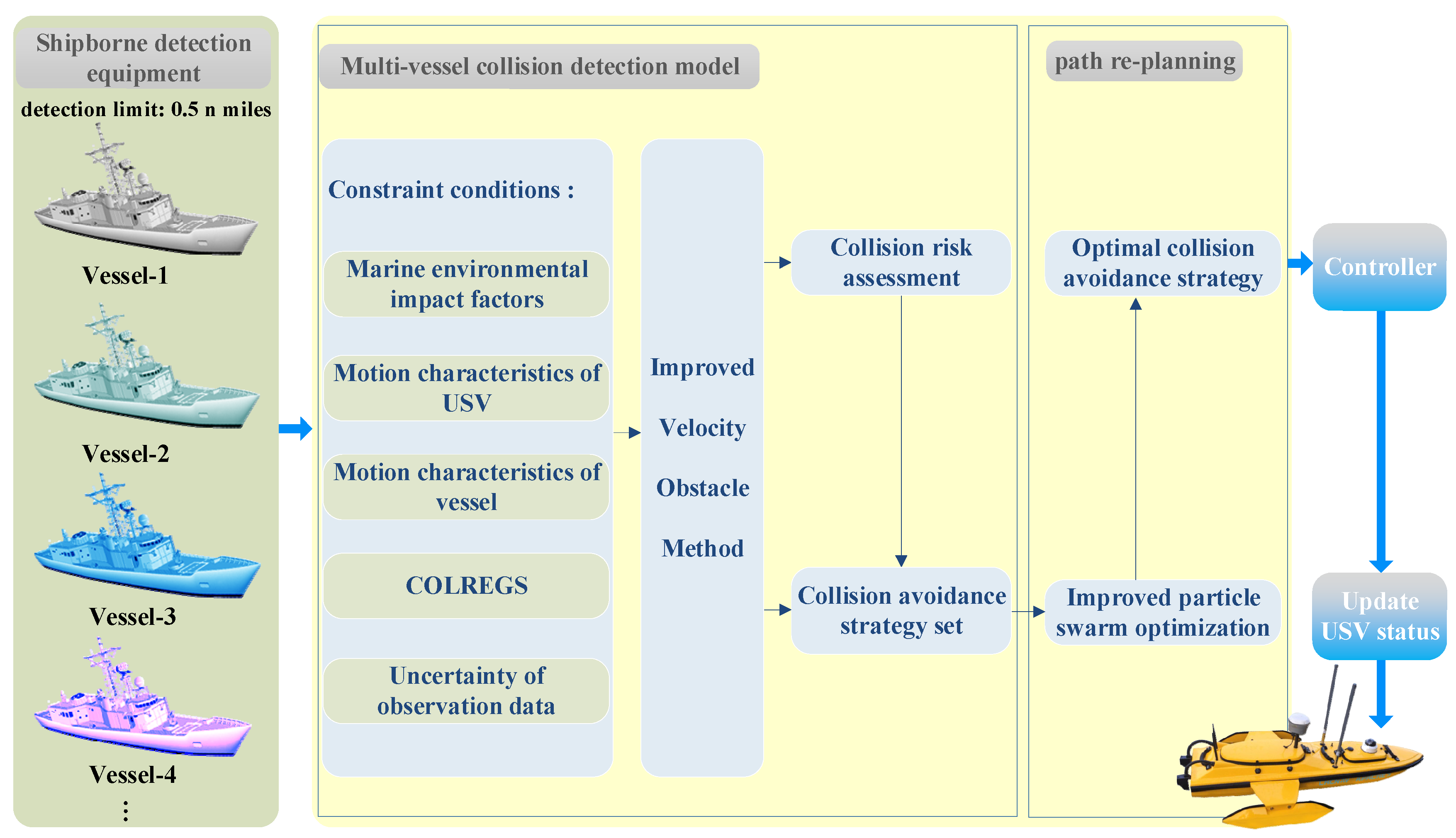
3.3. Multi-Vessel Encounters Collision Detection Model

The above model construction process is completed in an ideal state, ignoring COLREGS, the USV dynamic characteristics in the marine environment, and the encountering vessel motion characteristics; thus, this paper comprehensively considers the constraints of the above factors to construct the multi-vessel encounter collision detection model.

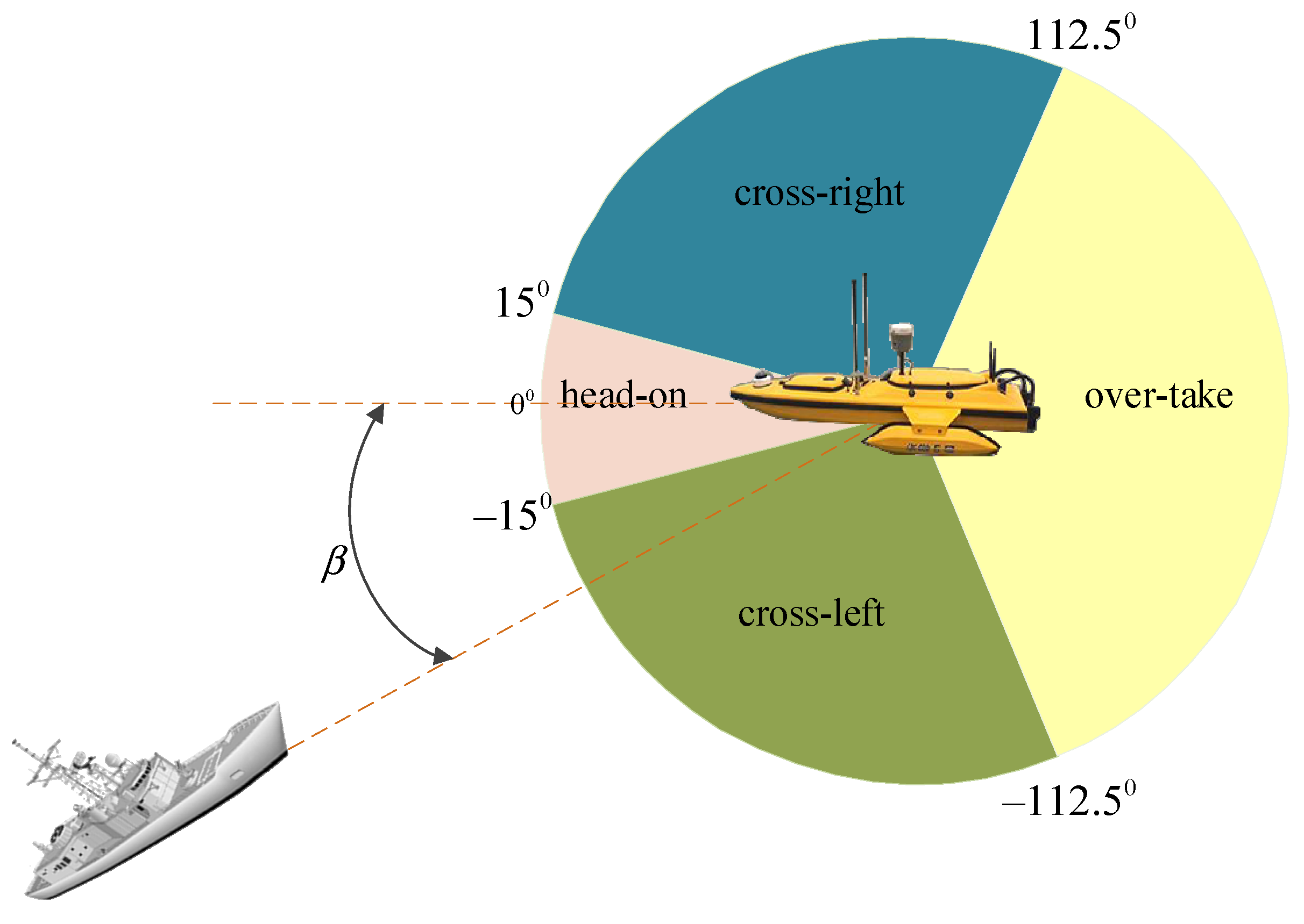
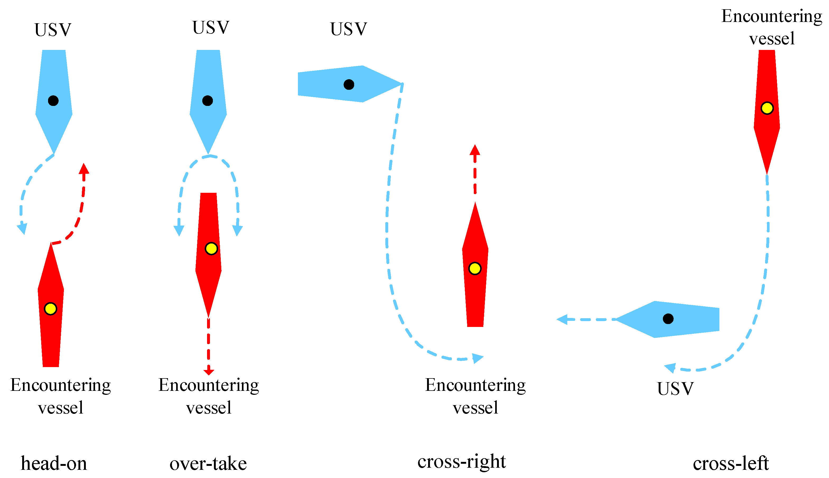
3.3.1. COLREGS and Model Definition of Multi-Vessel Encounters Scenario

There are usually three types of conflicts between USVs and encountering vessels: head-on scenarios, over-take scenarios, and cross scenarios. To ensure the safety of maritime navigation, USVs need to comply with COLREGS. COLREGS mainly distinguishes and defines encounter situations between ships according to the relative azimuth angle. The calculation formula for the relative azimuth angle is shown in Equation (12).

$$\beta =\mathrm{atan}\left(\frac{2\left(y_{USV}(t_k)-y_{Encounter-i}(t_k)\right)}{x_{USV}(t_k)-x_{Encounter-i}(t_k)}-{\psi }_{Encounter-i}(t_k)\right)$$

(12)

where $x_{USV}(t_k)$, $y_{USV}(t_k)$, $x_{Encounter-i}(t_k)$, and $y_{Encounter-i}(t_k)$ are the point coordinates of the USV and the encountering vessel at the time $t_k$. ${\psi }_{Encounter-i}(t_k)$ is the yaw angle of the encountering vessel.

After obtaining the relative azimuth $\beta$ between USV and the encountering vessel according to Equation (12), COLREGS defines the encountering scenario of the vessel as head-on, over-take, cross-right, and cross-left according to the relative azimuth $\beta$ of the encountering vessel. The partition expression and schematic diagram are shown in Equation (13) and Figure 5, respectively.

$$\{\begin{array}{ll}\beta \in \left[-{15}^{\circ },{15}^{\circ }\right)\hfill & \mathrm{USV} \mathrm{and} \mathrm{the} \mathrm{vessel} \mathrm{encountering} \mathrm{constitute} \mathrm{a} \text{head-on} \mathrm{scenario}\hfill \\ \beta \in \left[{112.5}^{\circ },{180}^{\circ }\right)\bigcup \left[-{180}^{\circ },-{112.5}^{\circ }\right)\hfill & \mathrm{USV} \mathrm{and} \mathrm{the} \mathrm{vessel} \mathrm{encountering} \mathrm{constitute} \mathrm{an} \text{over-take} \mathrm{scenario}\hfill \\ \beta \in \left[{15}^{\circ },{112.5}^{\circ }\right)\hfill & \mathrm{USV} \mathrm{and} \mathrm{the} \mathrm{vessel} \mathrm{encountering} \mathrm{constitute} \mathrm{a} \text{cross-right} \mathrm{scenario}\hfill \\ \beta \in \left[-{112.5}^{\circ },-{15}^{\circ }\right)\hfill & \mathrm{USV} \mathrm{and} \mathrm{the} \mathrm{vessel} \mathrm{encountering} \mathrm{constitute} \mathrm{a} \text{cross-left} \mathrm{scenario}\hfill \end{array}$$

(13)

The constraints of the COLREGS rules on the obstacle avoidance behavior of USVs are shown in

Table 1. COLREGS that USV should abide by in different multi-vessel encounters scenarios.

Encounters Scenario	COLREGS That USV Should Abide By	COLREGS That the Encountering Vessel Should Abide By
Head-on	USV is the avoiding party: Steering right past the starboard side of the encountering vessel.	The encountering vessel is the avoiding party: Steering right past the starboard side of USV.
Over-take	USV is the avoiding party: Steering right past the starboard side of the encountering vessel or steering left past the port side of the encountering vessel.	The encountering vessel will keep its current sailing status until the threat is lifted.
Cross-right	USV is the avoiding party; Slow down and steer right past the starboard side of the encountering vessel.	The encountering vessel will keep its current sailing status until the threat is lifted.
Cross-left	USV will keep its current sailing status until the threat is lifted.	The encountering vessel is the avoiding party:
		Take corresponding obstacle avoidance measures based on the encounter scenarios formed by USV and the encountering vessel.

, while the obstacle avoidance model is shown in Figure 6.

3.3.2. Collision Detection Model Construction

By the description given in Section 3.2, it can be seen that by changing the control input $\mathit{u}$ to change the motion state of USVs under the consideration of the USV dynamic characteristics and marine environmental factors, the waypoint of the USV is changed so that $P_{USV}(t_k)$ is far from $P_{Encounter-i}(t_k)\oplus ConfP$ and the USV can avoid vessels.

Equation (7) is nonlinear and it needs to use Runge–Kutta integration and the Taylor expansion law to approximate the state of the USV. The relationship between the system state and control input at time $t_k$ can be obtained:

$$\begin{array}{cc}X(t_k)& \approx {\displaystyle {\int }_{t_{k-1}}^{t_k}f\left(X(t_{k-1}),u(t_{k-1})\right)d{\tau }_{RB}}+{\displaystyle {\int }_{t_{k-1}}^{t_k}\left(\dot{X}(t_k)-\dot{\mathit{X}}(t_{k-1})\right)d{\tau }_{RB}}+{\displaystyle {\int }_{t_{k-1}}^{t_k}{\left[\left[\begin{array}{cc}\begin{array}{l}I\\ 0\end{array}& \begin{array}{l}0\\ M\end{array}\end{array}\right]+Q{k}_{d}V\right]}^{-1}Q{\tau }_{ED}d{\tau }_{ED}}\hfill \\ & =\tilde{\mathit{X}}(t_k)+G(t_k)\cdot \Delta u+B\hfill \end{array}$$

(14)

where $X(t_{k-1})$ and $u(t_{k-1})$ represent the system state of the USV and the control input at time $t_{k-1}$, respectively, and $\tilde{X}(t_k)$ represents the estimated system state of the USV at time $t_k$. $G\left(t\right)={\displaystyle {\int }_{t_{k-1}}^{t_k}{e}^{A\left(t-\tau \right)}Dd\tau }$, $A=\frac{\partial f}{\partial X}|{}_{X(t_{k-1}),u(t_{k-1})}$, $D=\frac{\partial f}{\partial u}|{}_{X(t_{k-1}),u(t_{k-1})}$, $\Delta u=u(t_k)-u(t_{k-1})$, $B={\displaystyle {\int }_{t_{k-1}}^{t_k}{\left[\left[\begin{array}{cc}\begin{array}{l}I\\ 0\end{array}& \begin{array}{l}0\\ M\end{array}\end{array}\right]+Q{k}_{d}V\right]}^{-1}Q{\tau }_{ED}d{\tau }_{ED}}$.

The relationship between the USV system state and its position at the time $t_k$ can be expressed as:

$$P_{USV}(t_k)=CX(t_k)$$

(15)

where $C=\left[\begin{array}{cc}\begin{array}{cc}\begin{array}{l}1\\ 1\end{array}& \begin{array}{l}1\\ 1\end{array}\end{array}& \begin{array}{cc}\begin{array}{l}0\\ 0\end{array}& \begin{array}{l}0\\ 0\end{array}\end{array}\end{array}\right]$. Substituting Equation (14) into Equation (15):

$$P_{USV}(t_k)=C\tilde{\mathit{X}}(t_k)+CG(t_k)\Delta u={\tilde{\mathit{P}}}_{USV}(t_k)+CG(t_k)\Delta u+CB$$

(16)

where ${\tilde{\mathit{P}}}_{USV}(t_k)$ represents the estimated position of USV at the time $t_k$.

According to Equations (8) and (16), the control input set that causes the USV to collide with the encountering vessel at a certain time in the future can be expressed as:

$$U{O}_{USV|Encounter-i}=\left\{\Delta u|\exists (t_k-t_{k-1})>0::\Delta u\in {\left(CG(t_k)\right)}^{-1}\left[\left(P_{Encounter-i}(t_k)-{\tilde{P}}_{USV}(t_k)-CB\right)\oplus ConfP\right]\right\}$$

(17)

To ensure that the obstacle avoidance behavior adopted by the USV satisfies the COLREGS rules, this paper divides the control input set $U{O}_{USV|Encounter-i}$ of the collision region based on the improved VO algorithm into four regions—namely, $U{O}_{USV|Encounter-i}$, $U{O}_{USV|left}$, $U{O}_{USV|right}$, and $U{O}_{USV|back}$. The expression is shown in Equation (18).

$$\{\begin{array}{l}U{O}_{USV|Encounter-i}=\left\{\Delta u|\exists (t_k-t_{k-1})>0::\Delta u\cdot P_{left}^{\perp }(t_k)\ge 0\bigcap \Delta u\cdot P_{right}^{\perp }(t_k)\ge 0\right\}\\ U{O}_{USV|left}=\left\{\Delta u|\exists (t_k-t_{k-1})>0::\Delta u\notin U{O}_{USV|Encounter-i}\bigcup U{O}_{USV|back}\bigcap \left[\Delta u\cdot \left(P_{USV}(t_k)-P_{Encounter-i}(t_k)\right)\right]<0\right\}\\ U{O}_{USV|right}=\left\{\Delta u|\exists (t_k-t_{k-1})>0::\Delta u\notin U{O}_{USV|left}\bigcup U{O}_{USV|back}\bigcup U{O}_{USV|Encounter-i}\right\}\\ U{O}_{USV|back}=\left\{\Delta u|\exists (t_k-t_{k-1})>0::\Delta u\cdot \left(P_{USV}(t_k)-P_{Encounter-i}(t_k)\right)<0\right\}\end{array}$$

(18)

where $P_{left}^{\perp }(t_k)$ and $P_{right}^{\perp }(t_k)$ are inward perpendicular to the left boundary and the right boundary of the geometric model of $U{O}_{USV|Encounter-i}$, respectively. The expressions are shown in Equation (19).

$$\{\begin{array}{l}{P}_{USV|left}^{\perp }(t_k)=\left[\begin{array}{l}\begin{array}{cc}\cos \left(-\mathit{\alpha }+\frac{\mathit{\pi }}{2}\right)& -\sin \left(-\mathit{\alpha }+\frac{\mathit{\pi }}{2}\right)\end{array}\\ \begin{array}{cc}\sin \left(-\mathit{\alpha }+\frac{\mathit{\pi }}{2}\right)& \cos \left(-\mathit{\alpha }+\frac{\mathit{\pi }}{2}\right)\end{array}\end{array}\right]\cdot \frac{P_{USV}(t_k)-P_{Encounter-i}(t_k)}{\Vert P_{USV}(t_k)-P_{Encounter-i}(t_k)\Vert }\\ P_{USV|right}^{\perp }(t_k)=J\left(\mathit{\alpha }-\frac{\mathit{\pi }}{2}\right)\left[\begin{array}{l}\begin{array}{cc}\cos \left(\mathit{\alpha }-\frac{\mathit{\pi }}{2}\right)& -\sin \left(\mathit{\alpha }-\frac{\mathit{\pi }}{2}\right)\end{array}\\ \begin{array}{cc}\sin \left(\mathit{\alpha }-\frac{\mathit{\pi }}{2}\right)& \cos \left(\mathit{\alpha }-\frac{\mathit{\pi }}{2}\right)\end{array}\end{array}\right]\cdot \frac{P_{USV}(t_k)-P_{Encounter-i}(t_k)}{\Vert P_{USV}(t_k)-P_{Encounter-i}(t_k)\Vert }\end{array}$$

(19)

where

$$\mathit{\alpha }=\arcsin \left(\frac{R}{\Vert P_{USV}(t_k)-P_{Encounter-i}(t_k)\Vert }\right)$$

(20)

where $U{O}_{USV|left}$ shows that the USV turning to the left side can enable it to avoid the solution set of the encountering vessel, $U{O}_{USV|right}$ shows that the USV turning to the right side can enable it to avoid the solution set of the encountering vessel, and $U{O}_{USV|back}$ shows the solution set of the USV backward avoidance of the encountering vessel.

To ensure the effectiveness of USV obstacle avoidance behavior, the motion state space of the USV obstacle avoidance behavior is obtained using the dynamic window method. The state space that the USV can reach from the current motion state through the time window:

$$W{D}_{USV}={\mathit{\nu }}_D=u_D={[u_D,v_D,r_D]}^{\mathrm{T}}$$

(21)

where

$$\begin{array}{c}{u}_D\in \left[u(t_k)-\dot{u}(t_k)\Delta t,u(t_k)+\dot{u}(t_k)\Delta t\right]\\ v_D\in \left[v(t_k)-\dot{v}(t_k)\Delta t,v(t_k)+\dot{v}(t_k)\Delta t\right]\\ r_D\in \left[r(t_k)\Delta t-\frac{1}{2}\dot{r}(t_k)\Delta t^2,r(t_k)\Delta t+\frac{1}{2}\dot{r}(t_k)\Delta t^2\right]\end{array}$$

(22)

where $u_D$, $v_D$, and $r_D$ represent the longitudinal velocity, transverse displacement velocity, and yaw angular velocity that the USV can reach within the time window $\Delta t$, respectively. $u(t_k)$, $v(t_k)$, and $r(t_k)$ represent the longitudinal velocity, transverse displacement velocity, and yaw angular velocity of the USV at the current moment, respectively. $\dot{u}(t_k)$, $\dot{v}(t_k)$, and $\dot{r}(t_k)$ represent the longitudinal acceleration, transverse acceleration, and yaw angle acceleration of the USV at the current time, respectively. Since the elements $W{D}_{USV}$ are continuous, they do not enable calculation in practical engineering. Therefore, the $W{D}_{USV}$ is discretized based on the principle of equal distance discretization, and the width of the discretization is M.

To ensure the enforceability of the collision avoidance strategy, two constraint conditions of the motion state space of the USV obstacle avoidance behavior and the velocity obstacle region are added to the dynamic window algorithm. The multi-vessel encounter collision detection model is shown in Figure 7. According to Equations (18) and (21), the obstacle avoidance strategy set ${\Omega }_{USV}$ for the USV that is achievable, safe, and compliant with COLREGS in the time window $\Delta t$ is shown in Equation (23):

$${\Omega }_{USV}=\{\begin{array}{ll}{S}_{right}& \beta \in \left[-{15}^{\circ },{15}^{\circ }\right)\\ S_{left}\bigcup S_{right}& \beta \in \left[{112.5}^{\circ },{180}^{\circ }\right)\bigcup \left[-{180}^{\circ },-{112.5}^{\circ }\right)\\ S_{right}& \beta \in \left[{15}^{\circ },{112.5}^{\circ }\right)\\ \Delta u=0& \beta \in \left[-{112.5}^{\circ },-{15}^{\circ }\right)\end{array}$$

(23)

where

$$\{\begin{array}{l}{S}_{left}=\left\{u|\left(u\in W{D}_{USV}\right)\bigcap \left(u\in U{O}_{USV|left}\right)\right\}\\ S_{rihht}=\left\{u|\left(u\in W{D}_{USV}\right)\bigcap \left(u\in U{O}_{USV|right}\right)\right\}\end{array}$$

(24)

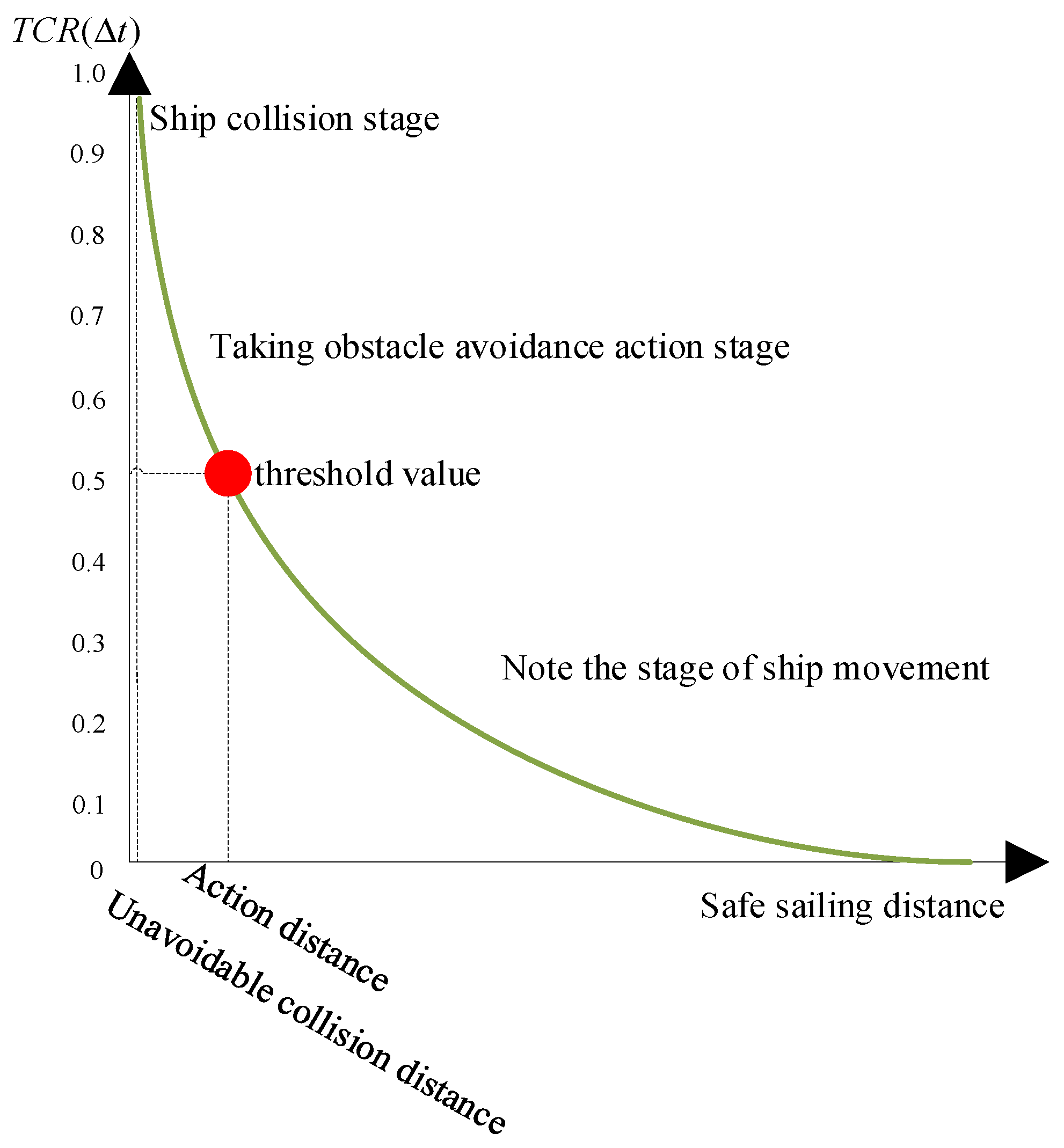
3.3.3. Construction of Collision Risk Assessment Model

For the timely and effective obstacle avoidance of the vessel, it is necessary to accurately assess the degree of collision threat of the vessel in the USV monitoring area. The collision risk assessment method proposed in reference [17] not only reflects the degree of danger when approaching the vessel but also reflects the difficulty of avoiding collision, as shown in Equation (25):

$$TCR\left(\Delta t\right)=\frac{N\left(S_c\right)}{N\left(S_c+{\Omega }_{USV}\right)}$$

(25)

where

$$S_c=\left\{u|\left(u\in W{D}_{USV}\right)\bigcap \left(u\in U{O}_{USV|Encounter-i}\right)\right\}$$

(26)

where $N(\cdot )$ represents the size of the collection area, which is obtained by Boolean operation. $TCR(\Delta t)$ represents the degree of threat to the USV caused by the encountering vessel, which is a measure of the possibility of collision between ships. The larger the evaluation value is, the fewer solutions are needed to avoid conflicts and the higher the collision risk, and vice versa. The corresponding threat level classification is shown in Figure 8.

It can be seen from Figure 8 that $TCR(\Delta t)$ is an important parameter for the USV to take obstacle avoidance action. This parameter uses the threshold to divide the action of USV in the scenario of multi-vessel encounters into two stages: paying attention to the encountering vessel movement trend and taking obstacle avoidance action. The threshold selected in this paper is 0.5; that is, when $TCR(\Delta t)\ge 0.5$, the USV needs to take obstacle avoidance action. In the scenario of multi-vessel encounters, the USV needs to sort the priority of the encountering vessel according to the size of the $TCR(\Delta t)$ value, and on this basis, obtain the opportunity to start the collision avoidance strategy according to the evaluation function introduced later, which provides an objective basis for the decision-making of the USV’s avoidance timing and avoidance priority.

4. Online Solution of USV Autonomous Obstacle Avoidance Model Based on Improved Particle Swarm Optimization

4.1. Optimal Collision Avoidance Strategy

The multi-vessel encounters collision detection model should quickly and accurately re-planning a safe and least resource cost-optimal path for the USV when USV shipborne detection equipment perceives the encountering vessel. In this paper, particle swarm optimization (PSO) is used to find the optimal collision avoidance strategy $u^{\ast }$ in the collision avoidance strategy set ${\Omega }_{USV}$.

The USV avoids obstacles by changing the control input $u$—that is, it changes longitudinal velocity $u$, transverse displacement velocity $v$, and yaw angular velocity $r$, so that the search space of the PSO algorithm has the dimension $d=3$. The updated formula for the particle velocity and position is shown in (27):

$$\{\begin{array}{l}{v}_i^{k+1}=\omega v_i^k+c_1{r}_1\left(pBes{t}_i^k-x_i^k\right)+c_2{r}_2\left(gBes{t}_i^k-x_i^k\right)\\ x_i^{k+1}=v_i^k+x_i^k\end{array}$$

(27)

where $v_i^k$ and $x_i^k$ represent the velocity and position of the particle $i\left(i=1,2,\dots ,m\right)$ in the kth iteration, respectively; $pBes{t}_i^k$ and $gBes{t}_i^k$ represent the individual optimal position and population optimal position searched for by particle $i$ and the whole particle population until the kth iteration, respectively; and $r_1$ and $r_2$ represent random numbers uniformly distributed in the interval $[0,1]$. $c_1$ and $c_2$ are normal numbers called learning factors. The larger $c_1$ is, the stronger the ability of particles to learn from their own historical experience is. The larger $c_2$ is, the stronger the degree of information sharing and collaboration between particles is. $\omega$ represents inertia weight. The larger this value is, the stronger the global search ability is; the smaller this value is, the stronger the local search ability is. These three parameters determine the ability of the particle to search for the optimal solution. The three parameters are improved below, and their expressions are shown in Equations (28) and (29).

$${\omega }_k=\left({\omega }_s-{\omega }_e\right)\ast \tan \left(\alpha \ast {\left(\frac{k_{\max }-k}{k_{\max }}\right)}^m\right)+{\omega }_e$$

(28)

$$\{\begin{array}{l}{c}_1=c_{1s}+\left(c_{1e}-c_{1s}\right)\ast k/k_{\max }\\ c_2=c_{2s}+\left(c_{2e}-c_{2s}\right)\ast k/k_{\max }\end{array}$$

(29)

In the early iteration of the PSO algorithm, the global search ability of particles is strong in order to detect the global space. In the late iteration of the PSO algorithm, particles need to strengthen their local search ability to search for the global optimal solution. Therefore, as the number of iterations increases, $\omega$ and $c_1$ should gradually decrease and $c_2$ should gradually increase. Here, $k$ is the current iteration number, $k_{\max }$ is the maximum iteration number, $\alpha =\pi /4$, ${\omega }_s=0.9$, and ${\omega }_e=0.4$. $m$ is the control factor, and its value is $0.5$. ${\omega }_k$ decreases linearly from $0.9$ to $0.4$ with the increase in the iteration number. $c_{1s}=2.5$, $c_{2s}=1.0$, $c_{1e}=1.0$, and $c_{2e}=2.5$. $c_1$ decreases nonlinearly from $2.5$ to $1.0$ with the increase in the iteration number, while $c_2$ increases nonlinearly from $1.0$ to $2.5$ with the increase in the iteration number.

The PSO algorithm evaluates the solution using the value of the fitness function. The fitness function is established on the premise of the minimum resource cost, as shown in Equation (30):

$$\min f\left({\Omega }_{USV}\right)={\epsilon }_1\cdot f_{dist}\left({\Omega }_{USV}\right)+{\epsilon }_2\cdot f_{heading}\left({\Omega }_{USV}\right)+{\epsilon }_3\cdot f_{velocity}\left({\Omega }_{USV}\right)$$

(30)

where $f_{dist}\left({\Omega }_{USV}\right)$, $f_{heading}\left({\Omega }_{USV}\right)$, and $f_{velocity}\left({\Omega }_{USV}\right)$ represent the path that is re-planned by USV during obstacle avoidance, the change in the yaw angle, and the change in the velocity, respectively. ${\epsilon }_1$, ${\epsilon }_2$, and ${\epsilon }_3$ are the corresponding weighting coefficients, and ${\epsilon }_1+{\epsilon }_2+{\epsilon }_3=1$. The shorter the re-planning path is, the smaller the USV energy consumption is. Meanwhile, a smaller amplitude of yaw angle and a smaller velocity change mean that the re-planning path will be smoother. The fewer times the yaw angle and velocity change, the lower the control cost will be. Therefore, the fitness function is selected in order to find the particle solution that can best minimize the fitness value in the PSO algorithm.

4.2. Realization of USV Autonomous Obstacle Avoidance Algorithm Based on Improved Velocity Obstacle Method

According to the algorithm description given above, the USV autonomous obstacle avoidance algorithm based on the improved velocity obstacle method is mainly realized through the following 11 steps, and the flow chart is shown in Figure 9.

• Step 1: The USV maintains the current state of motion and advances along the preset path. In real time, it senses the position, velocity, and water surface contours of the encountering vessel through the onboard detection sensors.
• Step 2: The velocity obstacle region $U{O}_{USV|Encounter-i}$ of the encountering vessel is constructed according to Equation (17). The solution set $U{O}_{USV|left}$ of the USV turning to the left to avoid the encountering vessel and the solution set $U{O}_{USV|right}$ of the USV turning to the right to avoid the encountering vessel are obtained so that USV can deal with emergent threats according to Equation (18).
• Step 3: The motion state-space $W{D}_{USV}$ of the USV is determined according to Equation (21) to ensure the effectiveness of the USV obstacle avoidance behavior.
• Step 4: Coupling steps 2 and 3 with COLREGS, the multi-vessel encounter collision detection model is constructed according to Equation (23), while the collision risk assessment model is constructed according to Equation (25).
• Step 5: If the collision threat degree of one or multiple vessels in the USV monitoring area is greater than the threshold $\left(TCR\left(\Delta t\right)\ge 0.5\right)$, then these vessels are determined to pose a threat to the USV. According to the $TCR(\Delta t)$ value, the obstacle avoidance priority of multiple vessels will be determined, and the obstacle avoidance strategy set ${\Omega }_{USV}$ with the highest priority will be generated. If the degree of collision threat to the vessel is less than the threshold $\left(TCR\left(\Delta t\right)<0.5\right)$, it is safe for the USV to continue sailing in its current state of motion.
• Step 6: The optimal collision avoidance strategy and the best starting time in the collision avoidance strategy set ${\Omega }_{USV}$ are found.
  • ① Initialize the parameters in the PSO algorithm: ${\omega }_s$, ${\omega }_e$, $c_{1s}$, $c_{1e}$, $c_{2s}$, and $c_{2e}$. The population size is $N$. The maximum number of iterations is $k_{\max }$; let $k=0$. Initialize the particle population—namely, the velocity and position of the particle. The historical optimal value of the individual particle is set to $pBest$, while the optimal value of the particle group is set to $gBest$.
  • ② In contemporary evolution, the fitness function $\min f\left({\Omega }_{USV}\right)$ for each particle is calculated according to Equation (30).
  • ③ Particles $pBest$ and $gBest$ are updated.
  • ④ The particles’ velocity and position are updated according to Equation (27).
  • ⑤ If the termination condition is satisfied, the output $gBest$ is the optimal collision avoidance strategy $u^{\ast }$; otherwise, return to ③.
• Step 7: Obstacle avoidance measures start to be taken. The optimal collision avoidance strategy $u^{\ast }$ needs to be input to the controller. the motion state of the USV is changed to ensure that the USV avoids the encountering vessel with the highest priority and the minimum control and energy consumption cost.
• Step 8: First, the highest priority vessel is avoided until the threat is lifted and then the sub-priority vessel is avoided. In turn, all encountering vessels are avoided in an orderly fashion.
• Step 9: If the collision threat of vessels in the USV monitoring area is less than the threshold $\left(TCR(\Delta t)<0.5\right)$, then the obstacle avoidance action ends.
• Step 10: Steps 2 to 9 are repeated at every interval $\Delta t$.
• Step 11: If USV arrives at the destination, the voyage ends; otherwise, it returns to the original path and continues to sail.

5. Simulation Analysis

5.1. Experimental Environment and Condition Assumptions

Using the MATLAB R2019a software, the performance of the proposed USV autonomous obstacle avoidance algorithm based on improved VO was tested to verify whether the re-planned obstacle avoidance path complies with COLREGS, meets the constraints of USV dynamics, and achieves the minimum control and energy consumption cost when avoiding vessels and returning to the original path. On this basis, through an experimental comparison with the USV autonomous obstacle avoidance algorithm based on VO and the USV autonomous obstacle avoidance algorithm based on SBG, the performance of the proposed USV autonomous obstacle avoidance algorithm based on improved VO was further analyzed to verify the security, timeliness, and economy of the algorithm. The experimental environment and assumptions were as follows:

• Preset global path waypoints. USV and the vessel move in a straight line at a uniform speed.
• The influence of the marine environment on the USV and the USV dynamic model are known. The parameter settings are shown in

  Table 2. USV performance parameters settings.

  Property	Value	Property	Value	Property	Value	Property	Value
  L [m]	8	$X_{\left|u\right|u}$	−1.327	$Y_{\left|v\right|r}$	−0.845	$N_{\dot{v}}$	0.000
  $m$	23.8	$X_{uuu}$	−5.866	$Y_{\left|v\right|v}$	−36.47	$N_{\dot{r}}$	−1.000
  $I_z$	1.760	$Y_v$	−0.889	$Y_{\left|r\right|v}$	−0.805	$N_{\left|v\right|r}$	0.0800
  $X_g$	0.046	$Y_{\dot{v}}$	−10.00	$Y_{\left|r\right|r}$	−3.450	$N_{\left|r\right|r}$	−0.750
  $X_u$	−0.723	$Y_r$	−7.250	$N_v$	0.0313	$N_{\left|r\right|v}$	0.130
  $X_{\dot{u}}$	−2.000	$Y_{\dot{r}}$	−0.030	$N_r$	−1.900	$N_{\left|v\right|v}$	3.9564

  and

  Table 3. Marine environment parameter settings.

  Property	Value
  The direction of the disturbances	240°
  Relative wind speed [m/s]	7.5
  Wave height [m]	2.5
  Relative ocean current [m/s]	2
  Area of frontal projection above the waterline [${\mathrm{m}}^2$]	330.9
  Area of lateral projection above the waterline [${\mathrm{m}}^2$]	874.8
  Area of frontal projection below the waterline [${\mathrm{m}}^2$]	91.0
  Area of lateral projection below the waterline [${\mathrm{m}}^2$]	323.4

  .
• This method uses the PD controller, $k_p=\left[200,200,10\right]$, $k_d=\left[5,5,5\right]$.
• The improved PSO algorithm is used to fins the optimal solution of the model, the number of particle populations $N=20$, and the maximum number of iterations $k_{\max }=180$.

5.2. Analysis of Simulation Results

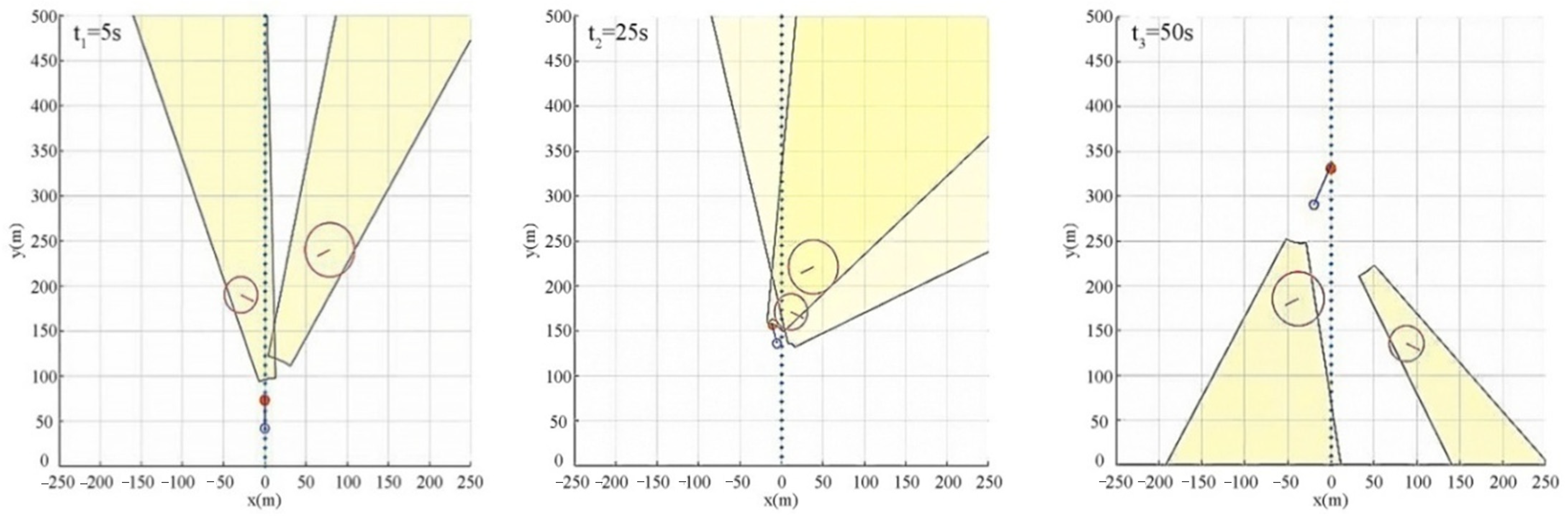
5.2.1. Algorithm Function Verification

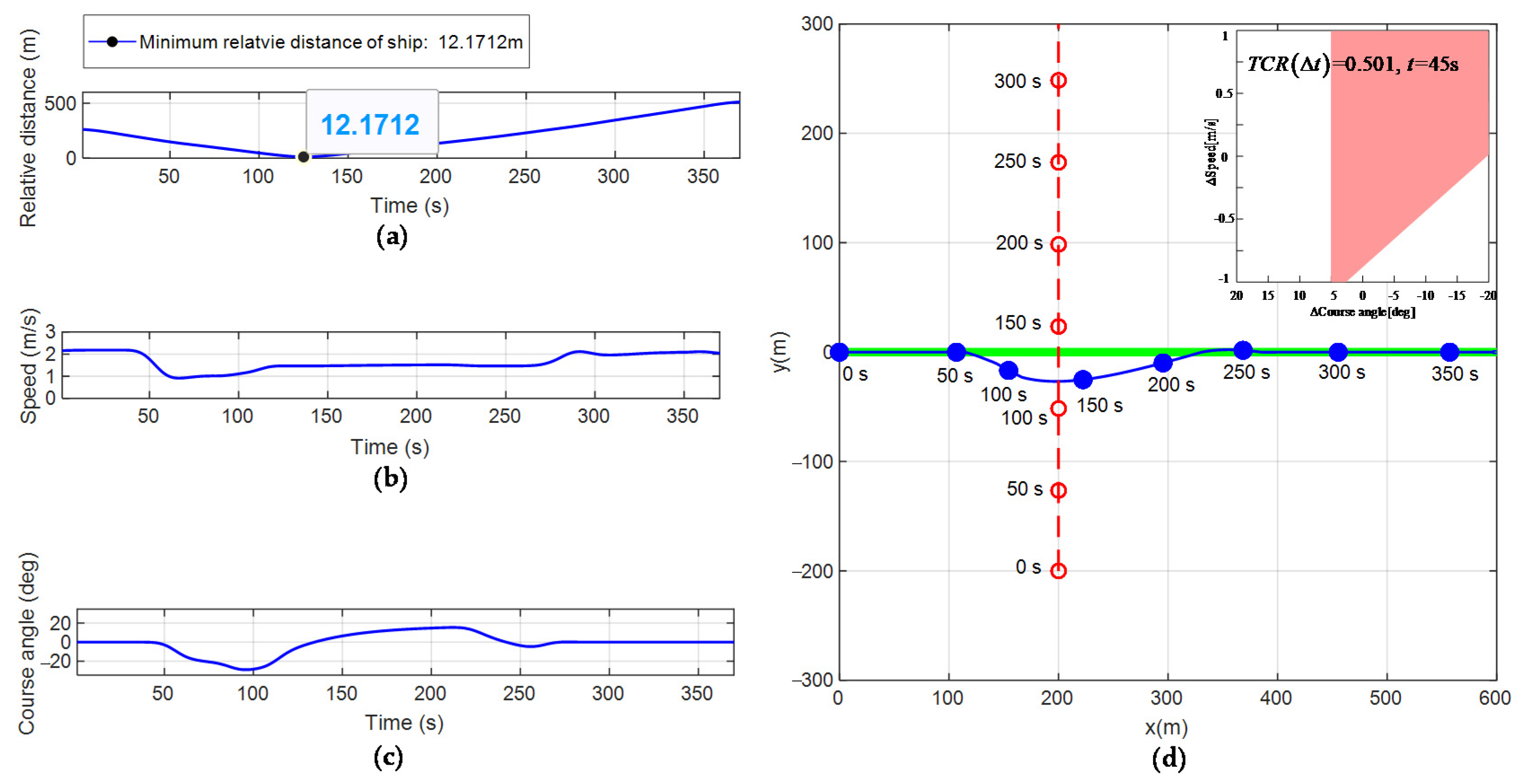
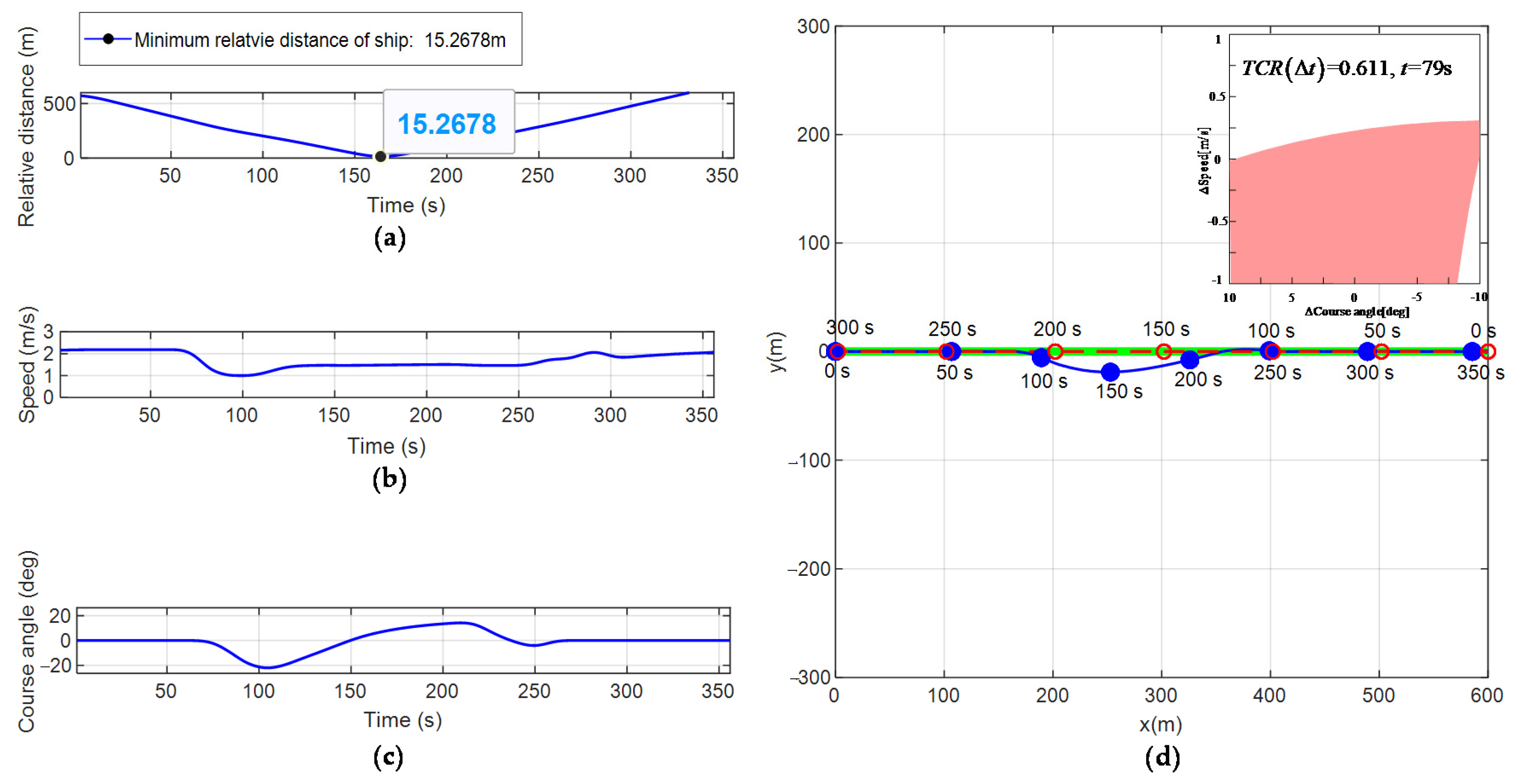
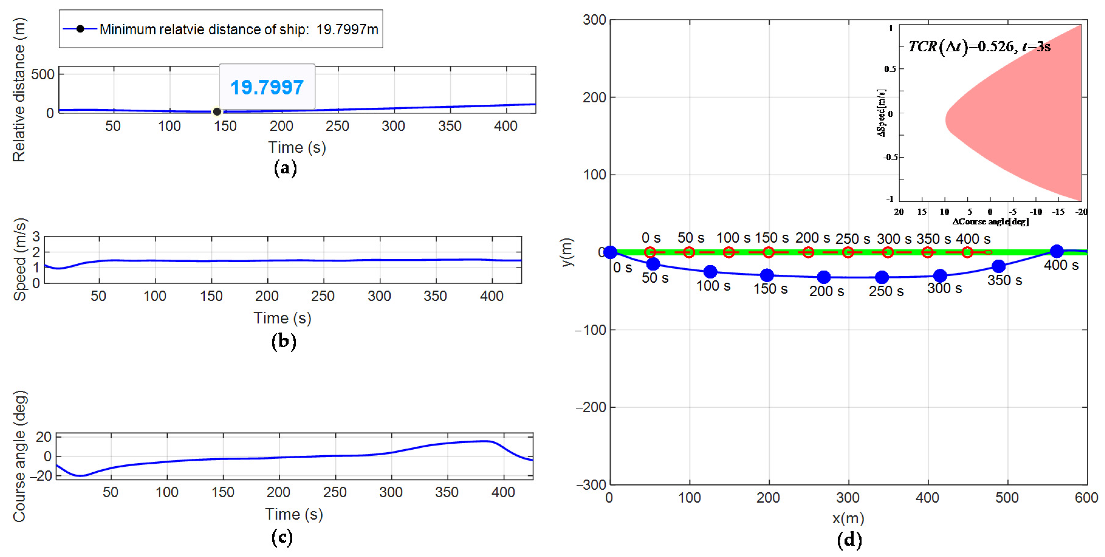
• In the scenario of a single-vessel encounter.

Firstly, the simulation simulates three scenarios of conflict between the USV and the encountering vessel: a cross-right scenario, a head-on scenario, and an over-take scenario. Whether the USV can abide by the COLREGS obstacle avoidance guidelines is verified by re-planning the path. The security, efficiency, and economy of the algorithm are analyzed through the collision threat degree, relative distance, velocity change, and yaw angle change. In the initial state, the parameter settings of the USV and the encountering vessel are shown in

Table 4. Settings of encounter scenario parameters.

Ship	Encounters Scenario	Initial Position [m]	Initial Velocity [m/s]	Initial Direction	Relative Azimuth Angle
USV	-	(0,0)	2	0°
Encountering vessel	Cross-right	(200, −200)	1.5	90°	90°
Encountering vessel	Head-on	(500, 0)	2	0°	0°
Encountering vessel	Over-take	(350, 0)	1	180°	180°

, and the simulation results are shown in

Table 5. Critical moment collision threat degree assessment results.

Collision Threat Degree	Timing of Obstacle Avoidance $\left(\mathit{t}=45 \mathbf{s}\right)$	Highest Collision Risk Moment $\left(\mathit{t}=135 \mathbf{s}\right)$
$TCR(\Delta t)$	$0.501$	$0.89$

,

Table 6. Critical moment collision threat degree assessment results.

Collision Threat Degree	Timing of Obstacle Avoidance $\left(\mathit{t}=79 \mathbf{s}\right)$	Highest Collision Risk Moment $\left(\mathit{t}=165 \mathbf{s}\right)$
$TCR(\Delta t)$	$0.611$	$0.86$

and

Table 7. Critical moment collision threat degree assessment results.

Collision Threat Degree	Timing of Obstacle Avoidance $\left(\mathit{t}=3 \mathbf{s}\right)$	Highest Collision Risk Moment $\left(\mathit{t}=148 \mathbf{s}\right)$
$TCR(\Delta t)$	$0.526$	$0.82$

and Figure 10, Figure 11 and Figure 12. In Figure 10, Figure 11 and Figure 12, the red hollow circle and the red dotted line track represent the running time and navigation path of the encountering vessel, respectively. The blue solid circle and the blue solid line track represent the running time and navigation path of the USV, respectively. The green solid line represents the global path of the USV.

Figure 10d simulates the obstacle avoidance process of the USV and the encountering vessel in the right-crossing encounter scenario. Figure 10a–c show the changes in the relative distance, velocity, and yaw angle of the USV over time during obstacle avoidance. Table 5 shows the real-time evaluation results of the collision threat of the encountering vessel in the USV monitoring area. The initial relative azimuth $\beta =90°$ of the two ships is within $[15°,112.5°)$. The two ships move forward in the initial direction linearly and the USV will enter a right-cross encounter situation with the vessel. According to the COLREGS rule, in the right-crossing encounter scenario, USV should slow down and steer right past the starboard side of the encountering vessel.

It can be seen from Table 5 that the USV runs to the 45th s and $TCR(\Delta t)=0.501$. Thus, the vessel will pose a threat to USV, and the behavior of the USV changes from the stage of paying attention to the movement of the encountering vessel to the stage of taking obstacle avoidance actions. The USV begins to follow its collision avoidance strategy by changing its velocity and yaw angle from the state of motion of the re-planned path. The USV runs to the 135th s and $TCR(\Delta t)=0.89$. At this time, the assessment value of the collision threat degree is the largest and the probability of a collision between two ships is the largest. Figure 10a shows that at the moment $t=135 \mathrm{s}$ when the risk of collision is the highest, the minimum relative distance between the two ships is 12.1712 m, which is greater than $ConfP$. Therefore, the USV can safely avoid the encountering vessel.

It can be seen from Figure 10b that the USV begins to take obstacle avoidance measures from the 45th s. The velocity of the USV decelerates from the initial value of 2 m/s to 1 m/s and then basically remains unchanged. This is the optimal collision avoidance strategy calculated by the evaluation function to prevent the USV from deviating too far from the original path. From the 100th s to the 135th s, the USV accelerates from 1 m/s to 1.25 m/s. This is necessary to ensure that the USV can pass the starboard side of the vessel. The encountering vessel moves uniformly and linearly, and its velocity and yaw angles remain unchanged. According to the relative distance between the two ships, if the USV is to pass the starboard side of the vessel, the USV needs to accelerate uniformly. According to the evaluation function, it needs to be accelerated to 1.25 m/s. From the 135th s to the 225th s, the velocity of the USV remains unchanged to enable the USV to return the original path with minimum control cost. After the USV successfully avoids the vessel, the relative distance between two ships becomes larger and larger, the probability of collision between two ships becomes smaller and smaller, and the USV begins to return to its original path. In accordance with the principle of minimum control cost, the USV changes its yaw angle and its velocity remains unchanged. From the 225th s to the 350th s, the velocity of the USV is unchanged after accelerating from 1.25 m/s to 2 m/s. This is because the obstacle avoidance action ends after the USV returns to the original path. To maintain the stability of the system, its velocity returns to the initial velocity and remains unchanged.

It can be seen from Figure 10c that the USV begins to change its yaw angle from the 50th s because the USV is affected by the rotation radius and its yaw angle cannot be changed immediately. From the 50th s to the 100th s, the USV abides by COLREGS to hit the rudder to the right. From the 100th s to the 135th s, the USV rudder returns to the center to ensure that the USV passes the starboard side of the vessel and does not deviate too far from the initial route. From the 135th s to the 225th s, the USV steers left, causing the USV to return to the original path with the minimum resource cost. From the 225th s to the 350th s, the rudder remains unchanged after returning to the middle. This is because after the USV returns to the original path, the obstacle avoidance action ends. To maintain the stability of the system, its yaw angle returns to the initial yaw angle and remains unchanged.

It can be seen from Figure 10d that the USV re-planning path is smoother, which satisfies the constraints of USV dynamics. The re-planning path does not deviate too far from the original path, which conforms to the USV minimum resource cost principle. During the USV obstacle avoidance process, the USV slows down and steers right, past the starboard side of the vessel. The USV successfully avoids the vessel by abiding by COLREGS.

Figure 11d simulates the obstacle avoidance process of the USV and the encountering vessel in a head-on encounter scenario. Figure 11a–c show the changes in the relative distance, velocity, and yaw angle with time in the obstacle avoidance process of the USV and the encountering vessel in the conflict scenario, respectively. Table 6 shows the real-time evaluation results for the degree of collision threat to the vessel in the USV monitoring area. Figure 12d simulates the obstacle avoidance process of the USV and the encountering vessel in the over-take encounter scenario. Figure 12a–c show the changes in the relative distance, velocity, and yaw angle with time in the obstacle avoidance process of the USV and the encountering vessel in the conflict scenario, respectively. Table 7 shows the real-time evaluation results for the degree of collision threat to the vessel in the USV monitoring area.

From the simulation results of Figure 11 and Figure 12, it can be seen that the obstacle avoidance process in both the head-on and over-take encounter scenarios is similar to that in the right-crossing encounter scenario shown in Figure 10. The USV adaptively selects the start time of obstacle avoidance through the real-time calculation $TCR(\Delta t)$ of the size. On this basis, under the constraints of the COLREGS rules and the USV dynamics and with achieving the minimum control cost and minimum energy consumption cost as the goal, the USV realizes efficient autonomous obstacle avoidance.

2.

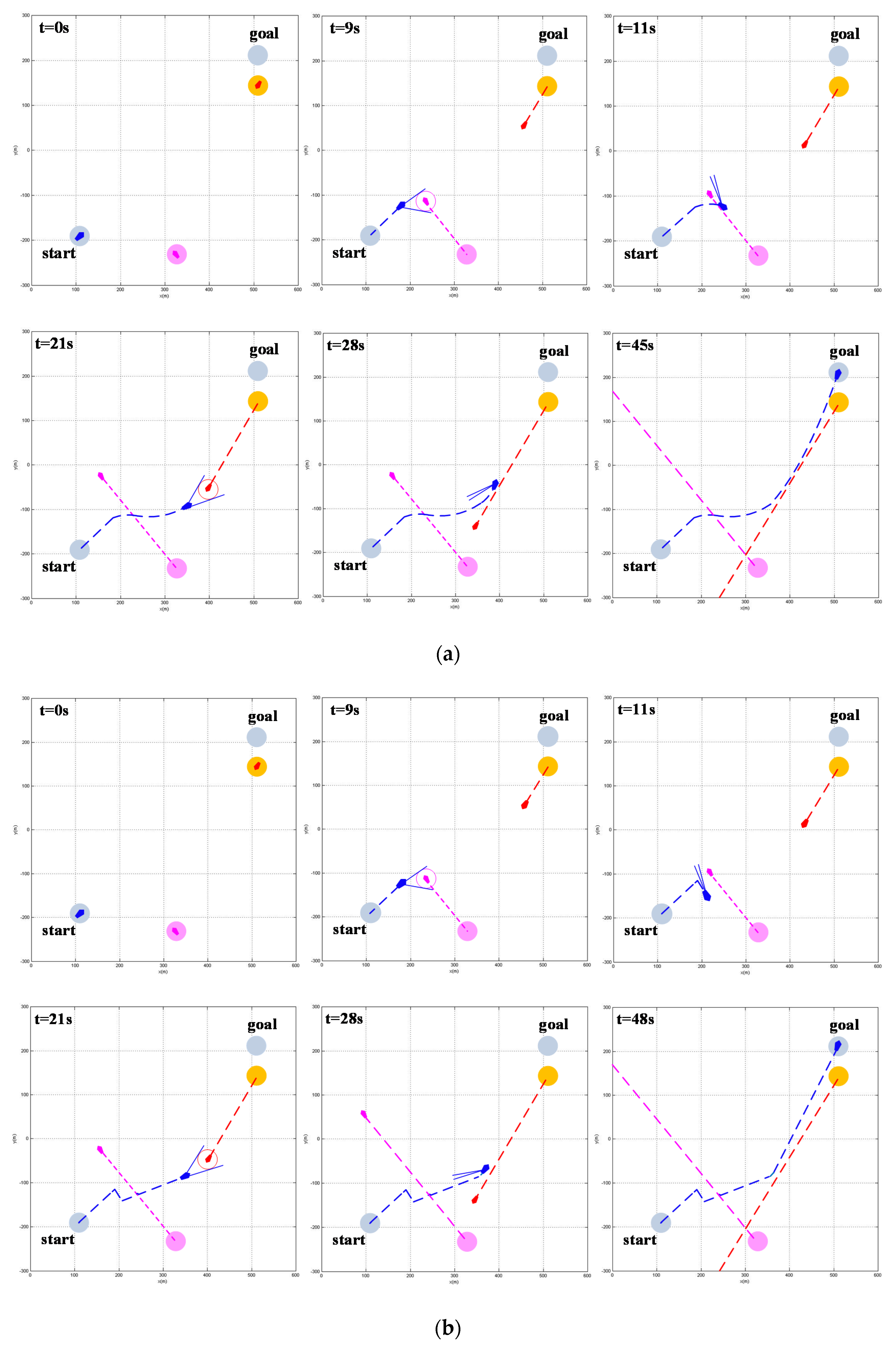
In the scenario of a multi-vessel encounter.

The effectiveness of the proposed algorithm is verified by simulating the USV autonomous obstacle avoidance process under multiple conflict scenarios between the USV and a single encountering vessel. Based on this, the autonomous obstacle avoidance process of the USV in the scenario of multi-vessel encounters is simulated to further verify the effectiveness of the proposed algorithm. The parameter settings for the multi-vessel encounter scenarios are shown in

Table 8. Settings of encounter scene parameters.

Ship	Encounter Situation	Initial Position [m]	Initial Velocity [m/s]	Initial Direction	Relative Azimuth Angle
USV		(0, 0)	2	0°	-
Encountering vessel 1	Over-take	(50, 0)	1	180°	180°
Encountering vessel 2	Cross-right	(200, −200)	1.5	90°	90°
Encountering vessel 3	Head-on	(500, −40)	1	0°	0°

, and the simulation results are shown in Figure 13. In Figure 13, the blue solid circle and the blue solid line trajectory represent the running time and navigation path of the USV, respectively, while the green solid line represents the global path of the USV. The red hollow circle and red dotted track represent the running time and navigation path of encountering vessel 1, respectively. The purple hollow circle and purple dotted track represent the running time and navigation path of encountering vessel 2, respectively. The rose-red hollow circle and rose red dotted track represent the running time and navigation path of encountering vessel 3.

Figure 13d simulates the obstacle avoidance process of the USV in the scenario of multi-vessel encounters. Figure 13a–c show the changes in the relative distance, velocity, and yaw angle of the USV over time during obstacle avoidance.

Table 9. Critical moment collision threat degree assessment results.

Critical Moment	$\mathit{T}\mathit{C}{\mathit{R}}_{\mathbf{s}\mathbf{h}\mathbf{i}\mathbf{p}1}$	$\mathit{T}\mathit{C}{\mathit{R}}_{\mathbf{s}\mathbf{h}\mathbf{i}\mathbf{p}2}$	$\mathit{T}\mathit{C}{\mathit{R}}_{\mathbf{s}\mathbf{h}\mathbf{i}\mathbf{p}3}$
Vessel 1 Start Obstacle Avoidance Time $\left(t_{\mathrm{ship}1}=3 \mathrm{s}\right)$	$0.636$	$0.502$	$0.195$
Vessel 1 Highest Threat Time $\left(t_{\mathrm{ship}1}=127 \mathrm{s}\right)$	$0.811$	$0.684$	$0.389$
Vessel 2 Start Obstacle Avoidance Time $\left(t_{\mathrm{ship}2}=131 \mathrm{s}\right)$	$0.493$	$0.712$	$0.437$
Vessel 2 Highest Threat Time $\left(t_{\mathrm{ship}2}=142 \mathrm{s}\right)$	$0.416$	$0.775$	$0.465$
Vessel 3 Start Obstacle Avoidance Time $\left(t_{\mathrm{ship}3}=150 \mathrm{s}\right)$	$0.359$	$0.486$	$0.521$
Vessel 3 Highest Threat Time $\left(t_{\mathrm{ship}3}=221 \mathrm{s}\right)$	$0.141$	$0.364$	$0.902$

shows the real-time evaluation results of the collision threat of the vessel in the USV monitoring area. The simulation scenario assumes that the USV travels to the target point along the global path of the initial plan and encounters three vessels, which move linearly, during the journey. Table 9 shows the real-time evaluation results for the collision threat of the vessel in the USV monitoring area.

It can be seen from Table 9 that when the USV runs to the 3rd s, the collision threat degrees of vessel 1, vessel 2, and vessel 3 are 0.66, 0.50, and 0.19, respectively. At this time, vessel 1 and vessel 2 pose a threat to the USV, but vessel 1 has the highest priority of obstacle avoidance. Therefore, the USV begins to take obstacle avoidance actions against vessel 1. The motion state is changed by changing the velocity and yaw angle to re-plan the path. When the USV runs to the 127th s, the probability of collision between USV and vessel 1 is the largest. At this time, the minimum relative distance between the two ships is 25.79 m, which is greater than $ConfP$. The USV successfully avoids vessel 1. The USV runs to the 131st s, $TC{R}_{\mathrm{ship}1}=0.493$, and the threat of vessel 1 to the USV is lifted. At this time, $TC{R}_{\mathrm{ship}2}=0.755$, $TC{R}_{\mathrm{ship}3}=0.437$, vessel 2 poses a threat to the USV, and the USV begins to take obstacle avoidance actions against vessel 2. When the USV runs to the 142nd s, the probability of a collision between the USV and vessel 2 is the greatest. At this time, the minimum relative distance between the two ships is 37.01 m, which is greater than $ConfP$. Thus, the USV successfully avoids vessel 2. As the USV runs to the 150th s, $TC{R}_{\mathrm{ship}2}=0.486$ and the threat of vessel 2 to the USV is lifted. At this time, $TC{R}_{\mathrm{ship}3}=0.521$, vessel 3 poses a threat to the USV, and the USV begins to take obstacle avoidance actions against vessel 3. When the USV runs to the 221st s, the probability of a collision between the USV and vessel 3 is the greatest. At this time, the minimum relative distance between the two ships is 11.91 m, which is greater than $ConfP$. Thus, the USV successfully avoids vessel 3. When the USV cannot detect any collision risk, the USV returns to the original route.

It can be seen from Figure 13d that the USV conducts path re-planning on the premise of complying with COLREGS. The re-planning path is smooth, which satisfies the constraints of the USV dynamics. The re-planning path does not deviate too far from the original path, meaning that it conforms to the USV minimum resource cost principle. Figure 13a–c show that the USV generates the collision avoidance strategy and navigation path executable by the control system on the premise of obtaining the minimum control cost.

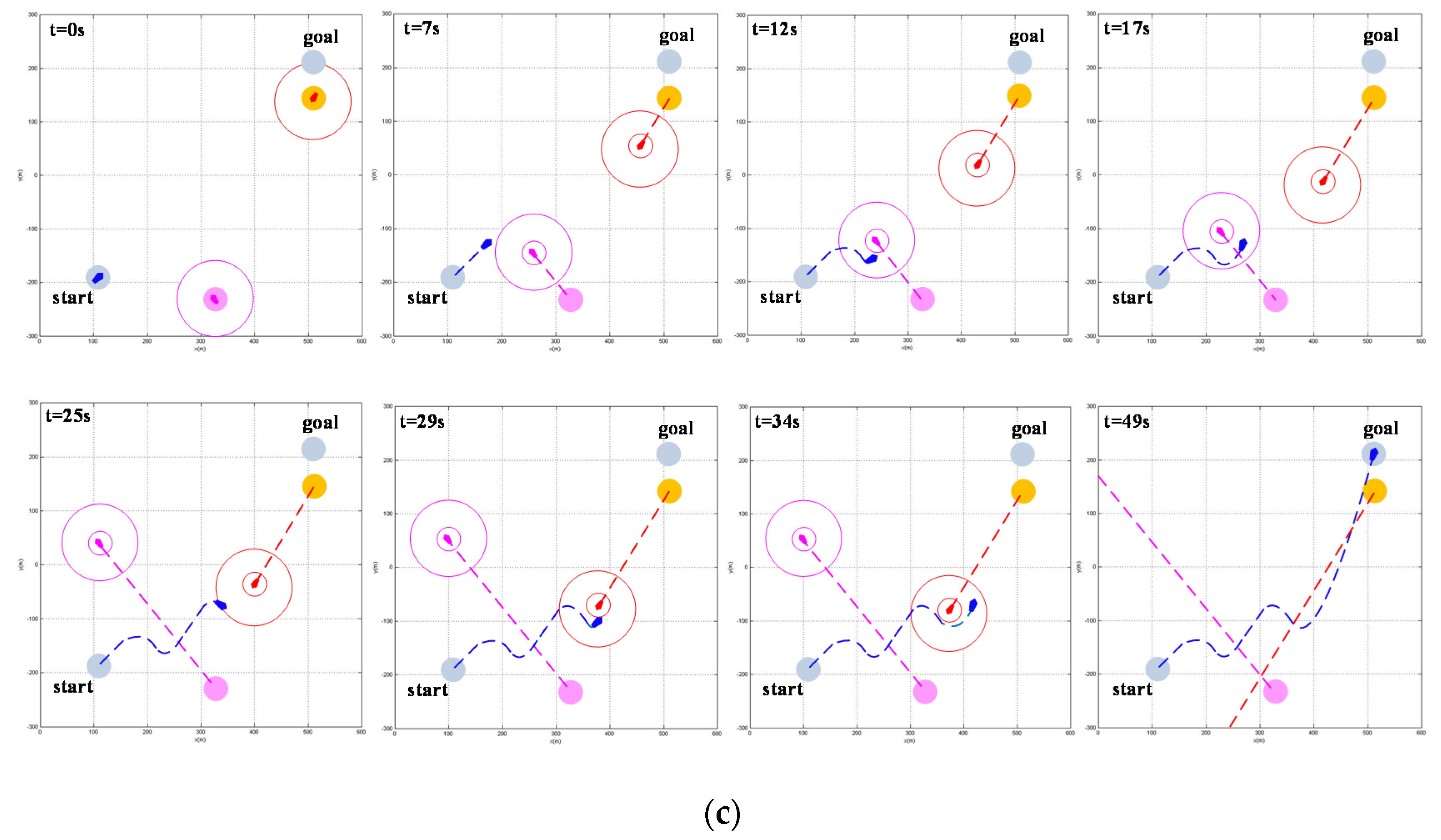
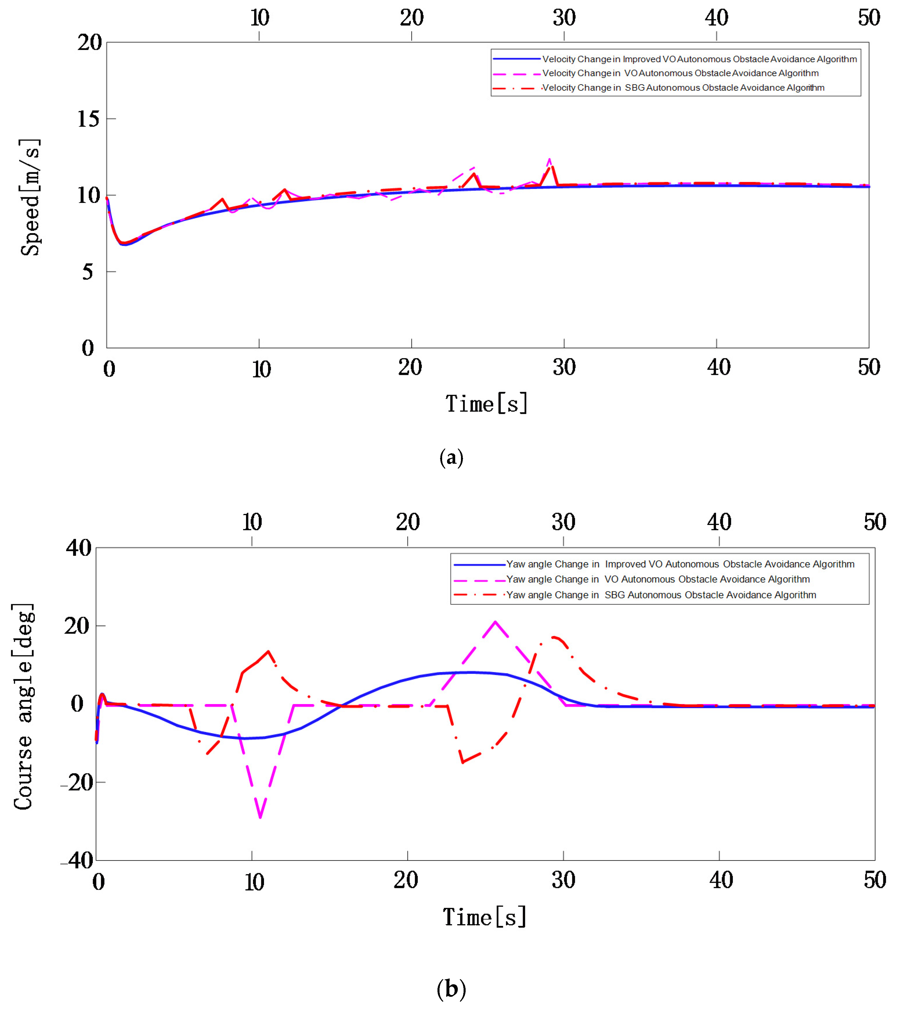
5.2.2. Algorithm Performance Verification

• Comparison and verification of the functional effectiveness of the three algorithms.

To verify the effectiveness of the algorithm proposed in this paper, we compare it with the autonomous obstacle avoidance method of the USV based on VO and the autonomous obstacle avoidance method of the USV based on SBG; thus, the performance of the proposed algorithm is further compared and verified. The simulation scenario assumes that the USV is sailing to the target point along the global path of the initial planning and encounters two vessels, which both move linearly toward their respective initial azimuths, during the journey. In the initial state, the parameter settings of the USV and the encountering vessel are shown in

Table 10. Settings of encounter scene parameters.

Ship	Encounter Situation	Initial Position [m]	Initial Velocity [m/s]	Initial Direction	Relative Azimuth Angle
USV		(0, 0)	10 m/s	45°
Encountering vessel 1	Head-on	(500, 0)	15 m/s	315°	90°
Encountering vessel 2	Over-take	(350, −0)	15 m/s	210°	−15°

and the simulation results are shown in Figure 14 and Figure 15. In Figure 14, the left lower blue circle and the right upper blue circle represent the starting point and the target point of the USV, respectively. The blue icon, red icon, and rose-red icon represent the USV, vessel 1, and vessel 2, respectively. The blue dotted track, the red dotted track, and the rose-red dotted track represent the navigation paths of the USV, vessel 1, and vessel 2, respectively. In Figure 15, the blue real line, the rose-red virtual line, and the red virtual line represent the simulation results obtained by the autonomous obstacle avoidance method of the USV based on improved VO, the simulation results obtained by the autonomous obstacle avoidance method of the USV based on VO, and the simulation results obtained by the autonomous obstacle avoidance method of the USV based on SBG, respectively.

Figure 14 simulates the obstacle avoidance process for the USV in the scenario of multi-vessel encounters. In the 9th s and the 21st s, both the obstacle avoidance method proposed in this paper and the obstacle avoidance method based on VO enable the USV to detect the vessel that poses a threat to it. In both, the USV needs to take two obstacle avoidance actions to complete the autonomous obstacle avoidance task. In the 7th s, the SBG-based obstacle avoidance method causes the USV to detect the collision alarm circle of vessel 1 and start to take obstacle avoidance actions. At the 11th s, it is necessary to change the collision avoidance strategy so that the USV can successfully avoid vessel 1. At the 25th s, the USV must detect the collision alarm circle of vessel 2 and start to take obstacle avoidance actions. At the 29th s, it is necessary to change the collision avoidance strategy so that the USV can successfully avoid vessel 2. This method necessitates two obstacle avoidance actions being taken to complete the autonomous obstacle avoidance task every time a vessel that poses a collision threat to the USV is detected. In this simulation, a total of four obstacle avoidance actions are taken to complete the autonomous obstacle avoidance task. Compared with the above two methods, this method has a greater control cost. In summary, the re-planning path of the obstacle avoidance method proposed in this paper is smoother and shorter; this means that the USV dynamic constraints are met and the minimum resource cost is achieved. The VO-based obstacle avoidance method re-planned the path to be sharper and longer, which did not fit with the physical motion characteristics of the USV. The obstacle avoidance method calculated by the SBG planned a smoother path but with a longer path length and a higher resource cost.

Figure 15a,b are schematic diagrams of the USV velocity changes and yaw angle changes during the autonomous obstacle avoidance process planned by three different algorithms. It can be seen from the figure that, compared with the other two algorithms, in the autonomous obstacle avoidance method for the USV based on improved VO, the change in amplitude of the velocity and yaw angle of the USV during obstacle avoidance is relatively small. However, the amplitude of the change in the yaw angle is slightly larger than that of the change in velocity. This is because this method takes full account of the USV dynamic characteristics, the encountering vessel motion characteristics, and the COLREGS rules during the obstacle avoidance process and uses the dynamic window to predict the velocity and yaw angle of the USV in real time. At the same time, to ensure that the USV can avoid encountering vessels in a timely and effective manner with the minimum obstacle avoidance cost, the USV responds preferentially by changing the yaw angle during obstacle avoidance. However, due to the coupling relationship between velocity and yaw angle, when the yaw angle changes the velocity will also experience some changes. In the autonomous obstacle avoidance method for the USV based on VO, in the process of obstacle avoidance the velocity and yaw angle change many times. Among these, the range of the velocity changes is relatively small, while the yaw angle range of change is relatively large, with two drastic changes. This is because this method regards the USV as a particle and does not evaluate the collision risk of the encountering vessel. If the velocity vector of the USV is within the velocity obstacle region of the encountering vessel, it will immediately change the yaw angle to keep it away from the velocity obstacle region. When the velocity vector of the USV is not in the velocity obstacle region of the encountering vessel, the velocity will become the initial velocity immediately. This not only leads to repeated changes in velocity and yaw angle, but also means that the velocity changes more frequently in this algorithm compared to the other two algorithms, as shown in Figure 15a. Different from the other two algorithms that take two obstacle avoidance measures to avoid colliding with two encountering vessels, the autonomous obstacle avoidance method for USVs based on SBG adopts four obstacle avoidance measures to avoid two encountering ships. This is because this method expands the ship domain model of the USV and establishes a conflict warning circle to perceive which vessel to avoid. When the USV detects the collision warning circle of the encountering vessel, it considers that the vessel poses a threat to the USV and starts to take obstacle avoidance measures to achieve large-scale obstacle avoidance. During the obstacle avoidance process, when the USV detects the ship domain model of the encountering vessel it will take obstacle avoidance measures again to carry out small-scale obstacle avoidance. Therefore, the method needs to take two obstacle avoidance actions to complete autonomous obstacle avoidance every time the vessel that poses a collision threat to the USV is detected. A total of four obstacle avoidance measures were taken for two encountering vessels and the velocity and yaw angle changed significantly four times, as shown in Figure 15a,b respectively.

2.

Comparison and verification of three algorithm performance indicators.

In order to verify the advantages and disadvantages of the three algorithms more clearly and intuitively, and based on the simulation experiment in Section 5.2.2 with Equation (30), the cost of the USV avoiding two encountering vessels is quantitatively compared. The results are shown in

Table 11. Comparison results of three algorithm performance indicators.

Encountering Vessel	Improved VO Autonomous Obstacle Avoidance Algorithm	VO Autonomous Obstacle Avoidance Algorithm	SBG Autonomous Obstacle Avoidance Algorithm
vessel 1	$f_{dist}\left({\Omega }_{USV}\right)=128.062$	$f_{dist}\left({\Omega }_{USV}\right)=159.193$	$f_{dist}\left({\Omega }_{USV}\right)=163.759$
	$f_{heading}\left({\Omega }_{USV}\right)=12.813$	$f_{heading}\left({\Omega }_{USV}\right)=27.174$	$f_{heading}\left({\Omega }_{USV}\right)=33.263$
	$f_{velocity}\left({\Omega }_{USV}\right)=3.752$	$f_{velocity}\left({\Omega }_{USV}\right)=14.069$	$f_{velocity}\left({\Omega }_{USV}\right)=8.515$
vessel 2	$f_{dist}\left({\Omega }_{USV}\right)=334.536$	$f_{dist}\left({\Omega }_{USV}\right)=361.019$	$f_{dist}\left({\Omega }_{USV}\right)=372.854$
	$f_{heading}\left({\Omega }_{USV}\right)=13.645$	$f_{heading}\left({\Omega }_{USV}\right)=21.731$	$f_{heading}\left({\Omega }_{USV}\right)=35.964$
	$f_{velocity}\left({\Omega }_{USV}\right)=0.037$	$f_{velocity}\left({\Omega }_{USV}\right)=9.925$	$f_{velocity}\left({\Omega }_{USV}\right)=4.156$
Total $f\left({\Omega }_{USV}\right)$ 1	$f\left({\Omega }_{USV}\right)=24.0187$	$f\left({\Omega }_{USV}\right)=46.1447$	$f\left({\Omega }_{USV}\right)=56.93406$

¹ $f\left({\Omega }_{USV}\right)$ is calculated according to Equation (30), where ${\epsilon }_1$, ${\epsilon }_2$, ${\epsilon }_3$ values are 0.01, 0.69, 0.3.

.

As can be seen from Table 11, in the process of obstacle avoidance for two encountering vessels among the three algorithms, the autonomous obstacle avoidance algorithm of USV based on improved VO has the smallest re-planning path length cost, cost of yaw angle change, and cost of velocity change, meaning that the total obstacle avoidance cost is also the smallest. This is because, in the process of avoiding obstacles using this method, the re-planning path is the shortest and smoothest and the velocity and yaw angle change most smoothly, as shown in Figure 14 and Figure 15, respectively. The total obstacle avoidance cost of the autonomous obstacle avoidance algorithm for USVs based on VO is the second lowest, while the total obstacle avoidance cost of the autonomous obstacle avoidance algorithm for USVs based on SBG is the largest. Thus, compared to the other two algorithms, the autonomous obstacle avoidance algorithm for USVs based on improved VO efficiently completes the autonomous obstacle avoidance of encountering vessels with the minimum obstacle avoidance cost.

6. Conclusions

This paper proposes a USV autonomous obstacle avoidance algorithm based on the improved VO method. The algorithm constructs a multi-vessel encounter collision detection model based on USV dynamic characteristics, vessels motion characteristics, and the COLREGS constraint model, thereby generating the velocity obstacle region and the USV executable collision avoidance strategy set. On this basis, the degree of collision threat to the vessel is calculated, which provides a decision basis for the USV to help it choose the time to start its collision avoidance strategy. At the same time, the path re-planning cost function is established to obtain the minimum resource cost and the improved particle swarm algorithm is used to hasten the solving speed of the model. Finally, a re-planning path in line with the dynamic characteristics of the USV is generated. In the simulation experiment, the effectiveness of the proposed method is verified by comparing it with the traditional VO-based autonomous obstacle avoidance method of USVs and the SBG-based autonomous obstacle avoidance method of USVs. The simulation results show that the algorithm can enable USVs to safely avoid multiple short-range dynamic targets under the influence of the marine environment. The generated path also meets the requirements of COLREGS.

References

1. Kum, B.C.; Shin, D.H.; Jang, S.; Lee, S.Y.; Lee, J.H.; Moh, T.; Lim, D.G.; Do, J.D.; Cho, J.H. Application of Unmanned Surface Vehicles in Coastal Environments: Bathymetric Survey using a Multibeam Echosounder. J. Coast. Res. 2020, 95, 1152–1156. [Google Scholar] [CrossRef]
2. Zhou, C.H.; Gu, S.D.; Wen, Y.Q.; Du, Z.; Xiao, C.S.; Huang, L.; Zhu, M. The review unmanned surface vehicle path planning: Based on multi-modality constraint. Ocean Eng. 2020, 200, 107046. [Google Scholar] [CrossRef]
3. Liu, Z.X.; Zhang, Y.M.; Yu, X.; Yuan, C. Unmanned surface vehicles: An overview of developments and challenges. Annu. Rev. Control 2016, 41, 737. [Google Scholar] [CrossRef]
4. Specht, M.; Specht, C.; Mindykowski, J.; Dąbrowski, P.; Maśnicki, R.; Makar, A. Geospatial Modeling of the Tombolo Phenomenon in Sopot using Integrated Geodetic and Hydrographic Measurement Methods. Remote Sens. 2020, 12, 737. [Google Scholar] [CrossRef] [Green Version]
5. Sang, H.; You, Y.; Sun, X.; Zhou, Y.; Liu, F. The hybrid path planning algorithm based on improved A* and artificial potential field for unmanned surface vehicle formations. Ocean Eng. 2021, 223, 108709. [Google Scholar] [CrossRef]
6. Woo, J.; Kim, N. Collision avoidance for an unmanned surface vehicle using deep reinforcement learning. Ocean Eng. 2020, 199, 107001. [Google Scholar] [CrossRef]
7. Li, C.Y.; Jiang, J.J.; Duan, F.J.; Liu, W.; Wang, X.Q.; Bu, L.R.; Sun, Z.B.; Yang, G.L. Modeling and Experimental Testing of an Unmanned Surface Vehicle with Rudderless Double Thrusters. Sensors 2019, 19, 2051. [Google Scholar] [CrossRef] [Green Version]
8. Stateczny, A.; Burdziakowski, P.; Najdecka, K.; Domagalska-Stateczna, B. Accuracy of Trajectory Tracking Based on Nonlinear Guidance Logic for Hydrographic Unmanned Surface Vessels. Sensors 2020, 20, 832. [Google Scholar] [CrossRef] [PubMed] [Green Version]
9. Liang, X.; Qu, X.; Hou, Y.; Li, Y.; Zhang, R. Distributed coordinated tracking control of multiple unmanned surface vehicles under complex marine environments. Ocean Eng. 2020, 205, 107328. [Google Scholar] [CrossRef]
10. Shah, B.C.; Gupta, S.K. Long-Distance Path Planning for Unmanned Surface Vehicles in Complex Marine Environment. IEEE J. Ocean Eng. 2020, 45, 813–830. [Google Scholar] [CrossRef]
11. Kurowski, M.; Thal, J.; Damerius, R.; Korte, H.; Jeinsch, T. Automated Survey in Very Shallow Water Using an Unmanned Surface Vehicle. IFAC PapersOnLine 2019, 52, 146–151. [Google Scholar] [CrossRef]
12. Mu, D.; Wang, G.; Fan, Y.; Qiu, B.; Sun, X. Adaptive Trajectory Tracking Control for Underactuated Unmanned Surface Vehicle Subject to Unknown Dynamics and Time-varing Disturbances. Appl. Sci. 2018, 8, 547. [Google Scholar] [CrossRef] [Green Version]
13. Song, A.L.; Su, B.Y.; Dong, C.Z.; Shen, D.W.; Xiang, E.Z.; Mao, F.P. A two-level dynamic obstacle avoidance algorithm for unmanned surface vehicles. Ocean Eng. 2018, 170, 351–360. [Google Scholar] [CrossRef]
14. Zhou, C.; Gu, S.; Wen, Y.; Du, Z.; Xiao, C.; Huang, L.; Zhu, M. Motion planning for an unmanned surface vehicle based on topological position maps. Ocean Eng. 2020, 198, 106798. [Google Scholar] [CrossRef]
15. Brushett, B.; Allen, A.; Futch, V. Implementation and Enhancement of Set-Based Guidance by Velocity Obstacle along with LiDAR for Unmanned Surface Vehicles. In Proceedings of the 2020 5th International Conference on Green Technology and Sustainable Development (GTSD), Ho Chi Minh City, Vietnam, 27–28 November 2020; Volume 198, p. 106798. [Google Scholar]
16. Battisti, T.; Muradore, R. A velocity obstacles approach for autonomous landing and teleoperated robots. Auton. Robots 2020, 44, 217–232. [Google Scholar] [CrossRef]
17. Yuan, X.; Zhang, D.; Zhang, J.; Zhang, M.; Soares, C.G. A novel real-time collision risk awareness method based on velocity obstacle considering uncertainties in ship dynamics. Ocean Eng. 2021, 220, 108436. [Google Scholar] [CrossRef]
18. Fiorini, P.; Shiller, Z. Motion Planning in Dynamic Environments Using Velocity Obstacles. Int. J. Robot. Res. 1988, 17, 760. [Google Scholar] [CrossRef]
19. Rufli, M.; Alonso-Mora, J.; Siegwart, R. Reciprocal Collision Avoidance with Motion Continuity Constraints. IEEE Trans. Robot. 2013, 29, 899–912. [Google Scholar] [CrossRef]
20. Snape, J.; Van Den Berg, J.; Guy, S.J.; Manocha, D. The Hybrid Reciprocal Velocity Obstacle. IEEE Trans. Robot. 2011, 27, 696–706. [Google Scholar] [CrossRef] [Green Version]
21. Gopalakrishnan, B.; Singh, A.K.; Kaushik, M.; Krishna, K.M.; Manocha, D. PRVO: Probabilistic Reciprocal Velocity Obstacle for Multi Robot Navigation under Uncertainty. In Proceedings of the 2017 IEEE/RSJ International Conference on Intelligent Robots and Systems (IROS), Vancouver, BC, Canada, 24–28 September 2017; Volume 27, pp. 696–706. [Google Scholar]
22. Bareiss, D.; Van den Berg, J. Generalized reciprocal collision avoidance. Int. J. Robot. Res. 2015, 34, 1501–1514. [Google Scholar] [CrossRef]
23. Huang, Y.; van Gelder, P.H.A.J.M. Time-Varying Risk Measurement for Ship Collision Prevention. Risk Anal. 2020, 40, 24–42. [Google Scholar] [CrossRef]
24. Kuwata, Y.; Wolf, M.T.; Zarzhitsky, D.; Huntsberger, T.L. Safe Maritime Autonomous Navigation with COLREGS, Using Velocity Obstacles. IEEE J. Ocean. Eng. 2014, 39, 110–119. [Google Scholar] [CrossRef]
25. Cho, Y.; Han, J.; Kim, J. Efficient COLREG-Compliant Collision Avoidance in Multi-Ship Encounter Situations. IEEE Trans. Intell. Transp. Syst. 2020, 20, 1–13. [Google Scholar] [CrossRef]
26. Zhu, X.; Yi, J.; Ding, H.; He, L. Velocity Obstacle Based on Vertical Ellipse for Multi-Robot Collision Avoidance. J. Intell. Robot. Syst. 2020, 99, 183–208. [Google Scholar] [CrossRef]
27. Singh, Y.; Sharma, S.; Sutton, R.; Hatton, D.; Khan, A. A constrained A* approach towards optimal path planning for an unmanned surface vehicle in a maritime environment containing dynamic obstacles and ocean currents. Ocean Eng. 2018, 169, 183–208. [Google Scholar] [CrossRef] [Green Version]
28. Bertaska, I.R.; Shah, B.; von Ellenrieder, K.; Švec, P.; Klinger, W.; Sinisterra, A.J.; Dhanak, M.; Gupta, S.K. Experimental evaluation of automatically-generated behaviors for USV operations. Ocean Eng. 2015, 106, 496–514. [Google Scholar] [CrossRef]
Figure 1. USV autonomous obstacle avoidance process in the scenario of multi-vessel encounters.
Ijgi 10 00618 g001
Figure 2. USV obstacle avoidance principle.
Ijgi 10 00618 g002
Figure 3. Velocity obstacle region based on VO model characterize.
Ijgi 10 00618 g003
Figure 4. USV autonomous obstacle avoidance process based on the VO method in the scenario of multi-vessel encounters.
Ijgi 10 00618 g004
Figure 5. Definition of multi-vessel encounters scenario.
Ijgi 10 00618 g005
Figure 6. Obstacle avoidance model under COLREGS.
Ijgi 10 00618 g006
Figure 7. Multi-vessel encounters collision detection model.
Ijgi 10 00618 g007
Figure 8. Threat level classification.
Ijgi 10 00618 g008
Figure 9. Implementation process of USV autonomous obstacle avoidance algorithm.
Ijgi 10 00618 g009
Figure 10. Obstacle avoidance process in the right cross encounter scenario. (a) Relative distance; (b) Change of velocity; (c) Change of yaw angle; (d) Obstacle avoidance process.
Ijgi 10 00618 g010
Figure 11. Obstacle avoidance process in the head-on encounter scenario. (a) Relative distance; (b) Change of velocity; (c) Change of yaw angle; (d) Obstacle avoidance process.
Ijgi 10 00618 g011
Figure 12. Obstacle avoidance process in the over-take encounter scenario. (a) Relative distance; (b) Change of velocity; (c) Change of yaw angle; (d) Obstacle avoidance process.
Ijgi 10 00618 g012
Figure 13. Obstacle avoidance process in the scenario of multi-vessel encounters. (a) Relative distance; (b) Change of velocity; (c) Change of yaw angle; (d) Obstacle avoidance process.
Ijgi 10 00618 g013
Figure 14. Obstacle avoidance process in the multi-vessel encounter situation: (a) Obstacle avoidance process based on improved VO autonomous obstacle avoidance algorithm; (b) Obstacle avoidance process based on VO autonomous obstacle avoidance algorithm; (c) Obstacle avoidance process based on SBG autonomous obstacle avoidance algorithm.
Ijgi 10 00618 g014aIjgi 10 00618 g014b
Figure 15. The schematic diagrams of USV velocity and yaw angle changes during autonomous obstacle avoidance with three algorithms. (a) Velocity Change of Autonomous Obstacle Avoidance Algorithm; (b) Yaw angle Change of Autonomous Obstacle Avoidance Algorithm.
Ijgi 10 00618 g015