
Application of Random Forest and SHAP Tree Explainer in Exploring Spatial (In)Justice to Aid Urban Planning


1
Department of Computer Science, Winston-Salem State University, Winston-Salem, NC 27110, USA
2
Center for Applied Data Science, Winston-Salem State University, Winston-Salem, NC 27110, USA
3
Department of History, Politics and Social Justice, Winston-Salem State University, Winston-Salem, NC 27110, USA
4
Spatial Justice Studio, Center for Design Innovation, Winston-Salem State University, Winston-Salem, NC 27110, USA
*
Author to whom correspondence should be addressed.
ISPRS Int. J. Geo-Inf. 2021, 10(9), 629; https://0-doi-org.brum.beds.ac.uk/10.3390/ijgi10090629
Submission received: 23 July 2021
/
Revised: 13 September 2021
/
Accepted: 16 September 2021
/
Published: 21 September 2021
Abstract
:In light of recent local, national, and global events, spatial justice provides a potentially powerful lens by which to explore a multitude of spatial inequalities. For more than two decades, scholars have been espousing the power of this concept to help develop more equitable and just communities. However, defining spatial justice and developing a methodology for quantitatively analyzing it is complicated and no agreed upon metric for examining spatial justice has been developed. Instead, individual measures of spatial injustices have been studied. One such individual measure is economic mobility. Recent research on economic mobility has revealed the importance of local geography on upward mobility and may serve as an important keystone in developing a metric for multiple place-based issues of spatial inequality. This paper seeks to explore place-based variables within individual census tracts in an effort to understand their impact on economic mobility and potentially spatial justice. The methodology relies on machine learning techniques and the results show that the best performing model is able to predict economic mobility of a census tract based on its spatial variables with 86% accuracy. The availability and density of jobs, compactness of the area, and the presence of medical facilities and underground storage tanks have the greatest influence, whereas some of the influential features are positively while the others are negatively associated. In the end, this research will allow for comparative analysis between differing geographies and also identify leading variables in the overall quest for spatial justice.
1. Introduction
Spatial justice as a theoretical concept holds much promise for exploring, understanding, and solving issues of spatial inequality in a wide variety of landscapes [1]. According to Rocco, “Spatial Justice refers to general access to public goods, basic services, cultural goods, economic opportunity and healthy environments” [2]. Numerous scholars have used the concept to call for a more equitable future for millions of people across the globe, as a theory by which urban planners should create more spatially just cities and as a political agenda to drive social change [3,4]. Achieving a spatially just geography would be a means by which to address the inequitable distribution of public and private goods, services, and resources.
However, the ‘real world’ application of this concept leaves much to be desired. From questions about the definition of the term, to issues of tackling past, current, and/or future spatial injustices, to making the larger public aware of the concept and its potential, spatial justice as a working concept is still in its infancy. With this in mind, the goal of this paper is to advance our collective understanding of spatial justice as it relates to measuring geographic inequalities that could potentially aid urban planners and policy makes. It is critical to develop quantitative techniques through which spatial justice can be explored across a variety of geographic landscapes. This article aids this process by utilizing a combination of data science, machine learning techniques, and geospatial information to explore place-based variables that influence locational equity in order to make objective data-driven decisions on issues of spatial justice/injustice, to aid urban management and planning.
The uneven distribution of public and private goods and services across the urban landscape has created numerous issues for the larger society. From poor performing schools to issues of gentrification and to food insecurity, spatial inequalities have become a byproduct of the capitalistic, market-driven, private property economic system that has become common across the globe. Numerous scholars have explored these singular issues of spatial inequalities, including studies on education, health, housing, food, transportation, and parks [5,6,7,8,9,10]. However, little scholarship has been focused on exploring how these manifestations of spatial inequality collectively impact the assessment of well-being and quality of life.
The one exception has been recent research focused on exploring issues of economic mobility in the United States [11]. While not an outright measure of spatial (in)justice, the examination of intergenerational economic mobility is rooted in many factors that are, at their core, spatial. Their study [11] on how a person’s probability of moving from the bottom 20% of the income ladder to the top in a generation revealed the importance of five factors: residential segregation, income inequality, primary school education, social capital, and family stability. Additionally, the study found that where one is born and raised has a causal effect on long-term economic outcomes. Being born on the “right” side of the tracks/river/highway can determine a person’s ability to reach higher income levels than his/her parents. Indeed, this research places local geography at the center of the debate regarding economic mobility [11].
The fact that local geography affects economic outcomes and quality of life is likely unsurprising to the millions of people who face an array of spatial injustices on a daily basis, which include unfair siting of environmental hazards, targeted school district assignments, and exclusionary zoning practices [1,12,13,14]. Hence, understanding the particular features of local geographies that either promote or hinder upward mobility is critical and has been the focus of recent studies. This paper is based on a comprehensive study and presents a data-driven approach that seeks to explore an array of place-based variables within individual census tracts in an effort to understand their impact on economic mobility and potentially on spatial justice. In the end, the goal is to allow for comparative analysis between differing geographies to assist urban management and planning and also identify leading variables in the overall quest for spatial justice.
Our previous research [15] began this process by utilizing a combination of data science and machine learning techniques and geospatial information to identify and explore a set of place-based variables that influence upward mobility, and spatial justice correspondingly. Results of our previous work showed that several machine learning models, including Random Forest (RF) Classifiers [16], were successful in finding complex underlying relationships between the selected spatial features and spatial (in)justice. This article is a continuation and refinement of our previous work with the additional goal of investigating interpretability [17] of the complex non-linear models in order to determine why the model makes certain predictions about spatial (in)justice, which place-based factors mostly influence the prediction, and how. Recent studies made significant progresses on exploring the interpretability of machine learning models [18,19,20] using local approximations and game theories; however, no studies have explored such interpretations in the context of economic mobility or spatial justice. To this end, this paper explores the behavior of the spatial features in predicting spatial justice using SHapley Additive exPlanations (SHAP) [20,21]. SHAP is useful in explaining various supervised learning models and assigns an importance value for each input feature for a specific prediction, which explains the root causes behind each prediction and therefore enhances transparency and reliability of a model.
The purpose of the research conducted in this article is to begin the development of a spatial justice index that will allow for comparative analysis between differing geographies and identify leading variables in the search for spatial justice. The analysis shows that it is possible to begin to develop a more robust and comprehensive spatial justice metric through the inclusion of the most critical locational variables in determining how “just” a local landscape may be. The spatial justice index is envisioned to be a metric that can be used to quantitatively compare diverse geographies based upon the level of spatial (in)justice at each location. Through the development of a spatial justice index, planners, public officials, policy makers, activists, concerned residents, etc. will be armed with a new tool to fight spatial injustices facing communities across the globe.
The rest of this article is organized as follows. Section 2 discusses background and related works, then Section 3 elaborates materials including study area, dataset, and preprocessing techniques utilized. Section 4 discusses the methodologies, Section 5 presents the results, and Section 6 focuses on discussing the results. Section 7 concludes the paper.
2. Background and Related Works
While not explicitly called “spatial justice”, the theoretical concept of prioritizing the geography of justice has been around for several decades and finds its modern-day roots in the work of Lefebvre, Harvey, and Pirie [22,23,24]. Lefebvre developed a concept called the “right to the city”, in which he calls upon society to reclaim the city for “all” in the face of increasing levels of commercialization, privatization and public-private partnerships [22]. Harvey builds upon Lefebvre’s “right to the city” and believes that geography cannot remain disengaged, impartial and objective, when many ills confront cities across the planet. As a result, he calls on geographers and others to bring together spatial and social analysis to improve urban spaces [23]. Pirie discusses the idea of “territorial social justice” and is perhaps the first person to use the term spatial justice in an academic paper. He states that, “Surely it would be another string in their bow if geographers could answer questions such as these: is a person’s living at place x just? Is the spatial distribution of grocery stores just? Is the siting of some new airport just? Is the re-siting of the hospital just? Is the removal and rehousing of squatters just? These questions range over the justness of absolute and relative location as well as over the justness of processes of siting and relocation” [24].
However, a concrete definition is still being developed. In his book, Seeking Spatial Justice, Soja does a masterful job discussing the importance of spatial justice, applications of spatial justice, and the need for planners to engage in proactive spatial justice efforts, but his pivotal work leaves much to be desired as it relates to providing a concrete definition of spatial justice [1]. The closest Soja comes is an affirmation of what spatial justice should be is as follows: Justice has a geography and that the equitable distribution of resources, services, and access is a basic human right. Meanwhile, Rocco states that “Spatial Justice refers to general access to public goods, basic services, cultural goods, economic opportunity and healthy environments” [2]. This is similar to Soja’s idea, but with a little bit more detail.
In the absence of a fully formed and agreed upon definition, most scholars have opted to provide the characteristics that would help make a place more spatially just. These characteristics tend to focus on three fundamental components: access, equity, and opportunity. Soja was interested in how differing geographies have access, opportunities, and equity as they relate to resources and services. Rocco goes a step further and adds public goods, basic services, cultural goods, economic opportunity, and healthy environments to the list of features that the population should have equal access to, opportunities for, and equitable distribution of. Fainstein offers her own opinion on how planners can contribute to what she calls “The Just City” by focusing on three factors: democracy, diversity, and equity [25]. In the end, the concept of spatial justice and related ideas provides an interesting lens for exploring issues of geographic inequality.
In addition to defining the term spatial justice, an important consideration is how to measure it, specifically, which locational-based variables are worthy of study. As stated above, individual studies of spatial injustices are quite common. These studies exploring spatial inequalities across geographies focus on environmental injustices, education, healthcare, transportation, and parks, to name a few [5,6,8,9,10,12]. However, they do not provide a complete picture of the spatial injustices that may be occurring at local geographies, and this paper seeks to begin developing a more robust and holistic exploration of spatial injustices in the belief that communities that suffer from one spatial injustice often have additional underlying concerns of injustice.
Recent academic research into economic mobility may provide an opportunity to bridge the gap that exists in the literature and begin the process of understanding the complex relationship numerous factors have on creating spatial injustices for certain communities. Reference [11] highlights the importance of place on economic mobility for the poorest populations in the United States [11]. Specifically, Chetty et al. explored a wide variety of place-based variables and the influence they have on economic opportunity for the poorest populations. In the end, their research found that place matters. Reference [26] determined that five factors are strongly correlated to these results: residential segregation, income inequality, school quality, social capital, and family structure. Several of these factors have a strong place-based component including residential segregation, income inequality, school quality, and social capital from which this study will build upon. Additionally, [26] stated the need for research on the relationship between economic mobility and location at “narrower geographies” in an effort to understand the microgeographic attributes that may influence economic mobility and in turn spatial injustices.
Researchers have identified many location-based factors relevant to economic mobility and as a result—potentially spatial justice, such as educational opportunities, de facto and de jure racism, quality of family networks, and specific geographic characteristics [27,28,29,30,31,32]. For example, [27] found a relationship between urban form and economic mobility. This work determined that the more compact a geographical area is, the higher upward economic mobility tends to be for residents in that area. In other words, sprawling built environments inhibit upward mobility and may play a role in exacerbating spatial inequalities. In the end, because of the diversity of variables that influence economic mobility, it provides a starting point for building a more robust model and understanding of spatial justice.
Inspired by the sporadic connections made by the previous research between location-based factors and economic mobility, the research presented in this paper aims to explore this relevancy in detail and utilizes a data science and machine learning-based approach to empirically evaluate the impact of place-based variables mentioned in Rocco’s framework on economic mobility and potentially spatial justice.
3. Materials
This section first details our study area geographically and spatially in Section 3.1. A list of features based on Rocco’s elaboration on spatial justice are identified and collected for each census tracts to create the dataset and is presented in Section 3.2. The dataset is further preprocessed to enforce standardization, balance, etc. and the steps are detailed in Section 3.3.
3.1. Study Area
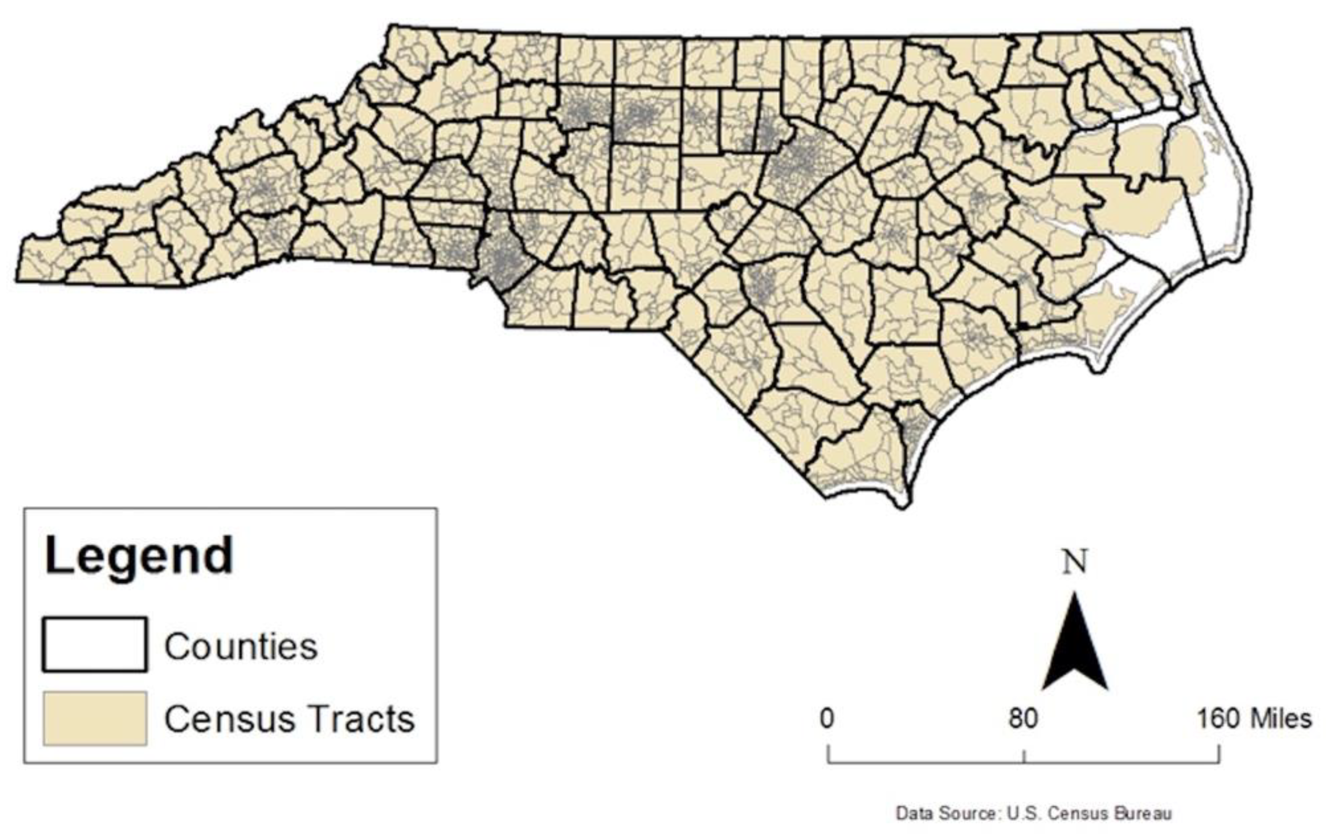
The presented study focuses on data acquired from 2157 census tracts within the USA state of North Carolina (NC). North Carolina is located along the eastern seaboard of the United States and is home to more than 10 million residents according to the most recent U.S. Census (2020 U. S. Census). Comprised of mountain, piedmont and coastal zones, North Carolina’s economy was originally agrarian in nature, which supported a large rural population. Beginning in the 1900’s North Carolina made a successful transition to a manufacturing economy (first) and more recently to a service/technology-based economy with a predominately urban population [33]. The State of North Carolina is divided into 100 counties and more than 500 municipalities that range in size from a few dozen to more than 800,000 residents (Charlotte, NC). The U.S. Census further divides the State into more than 2100 census tracts for statistical analysis purposes (Figure 1).
3.2. Dataset
The spatial feature set utilized in this study is constructed based on Rocco’s reference of spatial justice as general access to public goods, basic services, cultural goods, economic opportunity, and healthy environments. Table 1 provides an overview of Rocco’s characterization factors and corresponding spatial feature variables that were used in this study to measure them. The feature dataset is obtained from two primary sources. First, majority of the feature values were obtained from NC OneMap, a repository of geographic-based data located in the State of North Carolina [34], and were collected between 2018–2020. The NC OneMap website is the authoritative data collection for spatially based data in North Carolina and includes spatially referenced data on a multitude of categories including boundaries, community safety, education, environment, recreation and transportation. Some of the economic opportunity feature values such as Mean Travel Time to Work, Total Jobs, and Job Density were collected during 2015 and were obtained from reference [11]. Upward Economic Mobility, the outcome variable of interest for this study, is also calculated with reference [11]’s columns measuring income ranks for parents and children by census tract. More specifically, the target variable is calculated with income ranks for parents and children by census tract, and then is labeled as 0 when the difference between children and parents’ income is equal or less than zero (meaning no or downward economic mobility), and 1 for when the difference in income rank is positive (meaning upward economic mobility). Reference [11] provides these and other mobility statistics, collected during 2015, in the hopes that researchers will use them to further shed light on intergenerational income mobility at the local level. This research has adopted them as a surrogate for spatial justice at the census tract level.
3.3. Data Preprocessing
Once constructed, the dataset contains 2157 rows corresponding to NC census tracks with 28 numerical columns describing the spatial features as depicted in Table 1 and one binary target variable indicating Upward Mobility. During the preprocessing, the feature dataset is further explored for null values and outliers, and distribution of each feature column is explored. The data distribution reveals a large disparity in terms of scale among feature columns. To address this issue, the feature dataset is further normalized and standardized by utilizing python scikit-learns’ StandardScaler function to ensure all features have the same standard scale.
The constructed dataset is severely imbalanced; only 11% census tracts indicated Upward Mobility, while the rest demonstrated otherwise. The model based on this imbalanced dataset causes lower recall for minority class (Upward Mobility) and shows bias to the majority class (same or Downward Mobility). Several oversampling and undersampling strategies [35,36,37,38,39] are explored to address the imbalanced dataset such as synthetic minority oversampling technique (SMOTE) [36], near-miss algorithm [37], adaptive synthetic sampling (ADASYN) [38], and random undersampling [39]. Based on the experimental results and as suggested by the authors of SMOTE [36], a combination of SMOTE and random undersampling was utilized in this study to create a representative dataset. Unlike upsampling, which simply replicates duplicate samples, the SMOTE generates synthetic samples based on feature spaces that closely resemble the original dataset. The SMOTE was only applied to the training set in the cross-validation to avoid any possibility of overfitting. The performance of the model was evaluated using the test data set, which was never been exposed to the SMOTE or Random undersampling or cross validation.
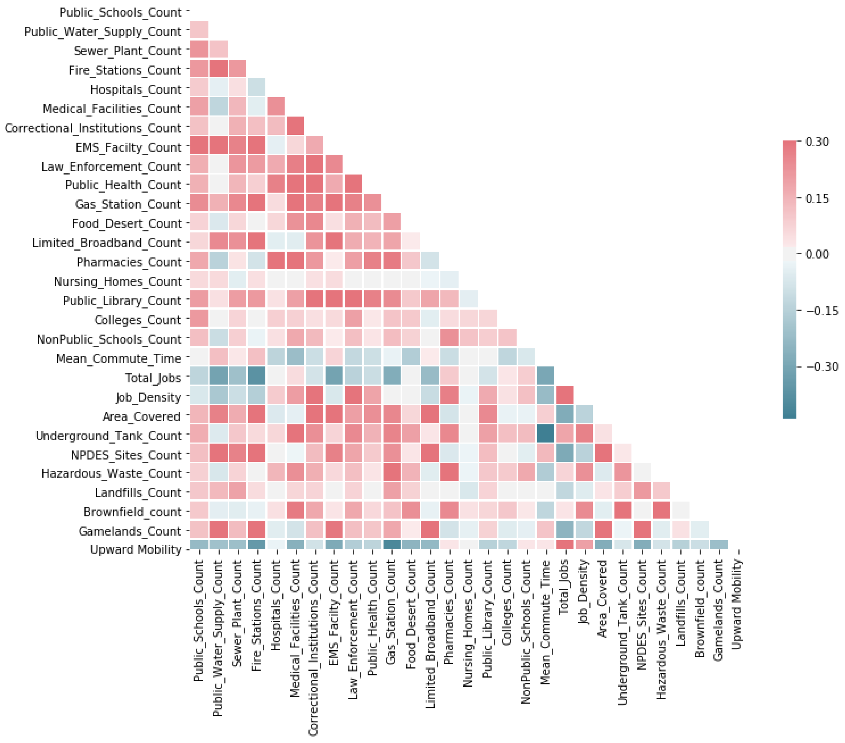
In order to better understand the effectiveness and adequacy of 28 spatial features in characterizing upward mobility, a correlation analysis is performed and the resultant correlation coefficients of all pairs of features is depicted in a color-coded plot, as in Figure 2. White encodes that the feature pair is not correlated, red indicates a positive correlation, and blue indicates a negative correlation. The darker a color, the larger the absolute correlation coefficient. For example, Figure 2 reveals that the features “Total_Jobs” and “Job_Density” are positively associated with the outcome variable “Upward Mobility”, whereas features such as “Fire_Stations_Count”, “Gas_Stations_count”, and “Area_Covered” are negatively correlated. With this plot, one can also spot a few highly correlated features that may represent similar and redundant place-based information. However, this research utilizes correlation analysis as an exploratory measure and chooses not to use correlation as a guideline for feature selection as two correlated features can still improve classification when they are in the same collection of features [40].
4. Methodology
The methodology is proposed according to the following two steps: first, a random forest (RF) classifier [16] with standard procedures of cross validation and hyperparameter tuning is detailed as an ideal candidate to make objective data-driven decisions on issues of spatial justice/injustice (Section 4.1). Second, the SHAP method [20,21] is elaborated in exploring interpretability of the RF model for identifying the contribution of various spatial features in determining various spatial justice outcomes (Section 4.2).
4.1. Classification Model
Our previous study utilized four different classifiers such as k-nearest neighbor (KNN), support vector machine (SVM), random forest (RF), and deep neural network (DNN) in classifying upward economic mobility based on the spatial features. Results of that study showed the superiority of RF and DNN classifiers over others. For this study, we focused on perfecting the RF algorithm with standard procedures of cross validation and hyperparameter tuning considering its overall predictive performance and computational cost of model development.
4.1.1. Random Forest (RF) Classifier
Random forest [16] is an ensemble tree-based learning algorithm. The RF Classifier consists a set of decision trees, each of them built over a random extraction of the observations from the dataset and a random extraction of the features. Not every decision tree in the set utilizes all the features or all the observations in the training dataset, and this guarantees that the trees are less correlated and more independent, and therefore less prone to over-fitting. Each tree uses a sequence of yes–no questions based on a single or combination of features in order to divide the training observations. At each node, the tree divides the dataset into two buckets, each of them hosting observations that are more similar among themselves and different from the ones in the other bucket. Therefore, the importance of each feature is derived from how “pure” each of the buckets is. The most widely used impurity measure is the Gini impurity, which is also utilized in this study. The classifier aggregates the votes from different decision trees to decide the final class of the test object.
Compared with other classifiers that were explored in our previous study, RF has good and robust performance in prediction, owing to the ensemble mechanism. Because of the randomization in choosing the features to split, RF is also robust in the presence of uninformative and redundant features. This property is especially good for this research with the possible existence of a number of redundant (highly correlated to each other as explained in Section 3.1) features whose relative importance is not known beforehand. Another desirable property of RF is the insensitivity to outliers. As some census tracts may have extremely high values for some spatial variables, the expectation is that the RF will perform better in such cases. It also has relatively low computational cost because the training and testing of underlying decision trees are much more straightforward than optimization-based models such as neural network, support vector machine, etc. The low computational cost also makes it feasible to perform extensive searching for the optimal hyperparameters. Additionally, the tree-based structure of RF makes it transparent in making decisions, providing good interpretability, which was utilized to explain individual predictions, as elaborated in Section 4.2.
4.1.2. Cross Validation and Hyperparameter Tuning
Hyperparameters of the random search classification were tuned by utilizing both grid and random searches. First, a randomized parameter search with 5-fold cross-validation using python scikit-learns’ RandomizedSearchCV with 1000 iterations and 5000 fits were implemented. The range of best performing parameters from that search were then added to the GridSearchCV to find the optimized set of parameters through the parameter space. The best performing parameters were then implemented to the final model. After tuning, the maximum depth of the tree, the number of features to consider when looking for the best split, and the number of trees hyperparameters were set to 20, 10, and 300, respectively. The tuning method was time consuming, as it went through multiple searches through the parameter space; however, once tuned, the model was able to make more accurate predictions in a timely manner.
4.1.3. Classifier Performance Evaluation Metrics
The classifier performances are evaluated using various standard evaluation metrics such as Precision, Recall, Accuracy, F1, and ROC score. In this study, Precision is the ratio of correctly predicted Upward Mobility observations to the total predicted Upward Mobility observations. Recall is the ratio of correctly predicted Upward Mobility observations to all actual observations with Upward Mobility labels. Accuracy is the most intuitive measure depicted as the ratio of the correctly labeled observations to the whole pool of observations. F1 score takes both Recall and Precision into account, hence can be considered as a weighted average of them, and therefore it provides a useful accuracy indicator. The ROC curve is another common tool used with binary classifiers. The ROC curve plots the true positive rate (TPR, another name for Recall) against the false positive rate (FPR). The FPR is the ratio of negative instances that are incorrectly classified as positive.
4.2. Model Interpretability with SHAP
SHAP is a widely used approach for explaining machine learning models based on cooperative game theory [20]. The SHAP explanation method computes Shapley values from coalitional game theory, where the feature values of a data instance act as players in a coalition and Shapley values tell us how to fairly distribute the “payout” (=the prediction) among the features. This research utilized SHAP to analyze individual census tract sample predicted by the RF model in order to estimate how much each of the 28 features contributes to the spatially just vs. unjust predictions. More specifically, SHAP tree explainer [21], a version of SHAP for tree-based machine learning models (e.g., decision trees, random forest (RF), and gradient boosted trees) is adopted. The choice of SHAP to provide interpretability was driven by its ability to provide both global and local interpretability. Each observation can obtain its SHAP value, therefore the SHAP can help interpret the model globally as well as locally. Additionally, contrary to the existing methodologies for finding importance features in machine learning models, SHAP can identify whether the contribution of each input feature is positive or negative, which is critical for this research.
The analysis performed by the SHAP tool is useful on unfolding the “black box” nature of the RF classifier model in order to enhance model interpretability and possibility of real-life adoption in urban planning and management. More specifically, this research focuses on answering further important questions such as below by utilizing SHAP tool.
- (a)
- What are the most influential spatial features impacting the model output?
- (b)
- What are the characteristics of a space that exhibits upward mobility and spatial justice, respectively?
- (c)
- What are the characteristics for the spatially unjust places?
5. Results
5.1. Classification Results
This section details an empirical evaluation of different machine learning algorithms on spatial dataset. The experiments were set up using Python and TensorFlow libraries. The curated dataset was divided into training (75%) and testing (25%) sets, and were utilized during model training and classification, respectively. During the data split, stratified sampling was enforced to ensure that the right number of instances were sampled from each mobility subgroups to guarantee that the test set was representative of overall population. The training dataset was further divided into training and validation sets and were utilized during cross validation and hyperparameter tuning as elaborated in Section 4.1.2.
Table 2 shows the evaluation metrics of the RF classifier while comparing them with two additional classifiers (KNN and SVM) from our previous study, signifying its superiority. The training and testing accuracy for the RF model is 0.87 and 0.86, respectively, signifying that the model is not overfitted. The RF model was able to achieve 0.85 recall (Sensitivity), predicting 85% of all upward mobility test cases (minority class instances) correctly. The overall accuracy of the RF model is also relatively higher and indicates that there is enough variability in spatial dataset to potentially characterize upward mobility and in turn spatial justice. Figure 3 shows the ROC curves and the corresponding AUC values of all models. The ideal point in ROC space is the top-left corner. AUC is an important statistical parameter for evaluating classifier performance: the closer AUC is to 1, the better overall performance of established classifier. In the current work, as shown in Figure 2, the AUC value of the RF model is 0.858, which is higher than the other machine learning models by a significant margin (7% or more).
5.2. Model Interpretability and Feature Importance Results
The ultimate goal of this paper is to explore location-based variables that influence spatial justice in order to make objective data-driven decisions on issues of spatial (in)justice. The prediction results presented in the previous section based on the best performing RF model potentially suggests that the chosen array of spatial variables is capable of characterizing the upward mobility vs. no mobility, and in turn is able to predict spatially just vs. unjust places. This section of the article focuses on identifying most important features for the purpose of verifying the correctness and enhancing the interpretability of the model.
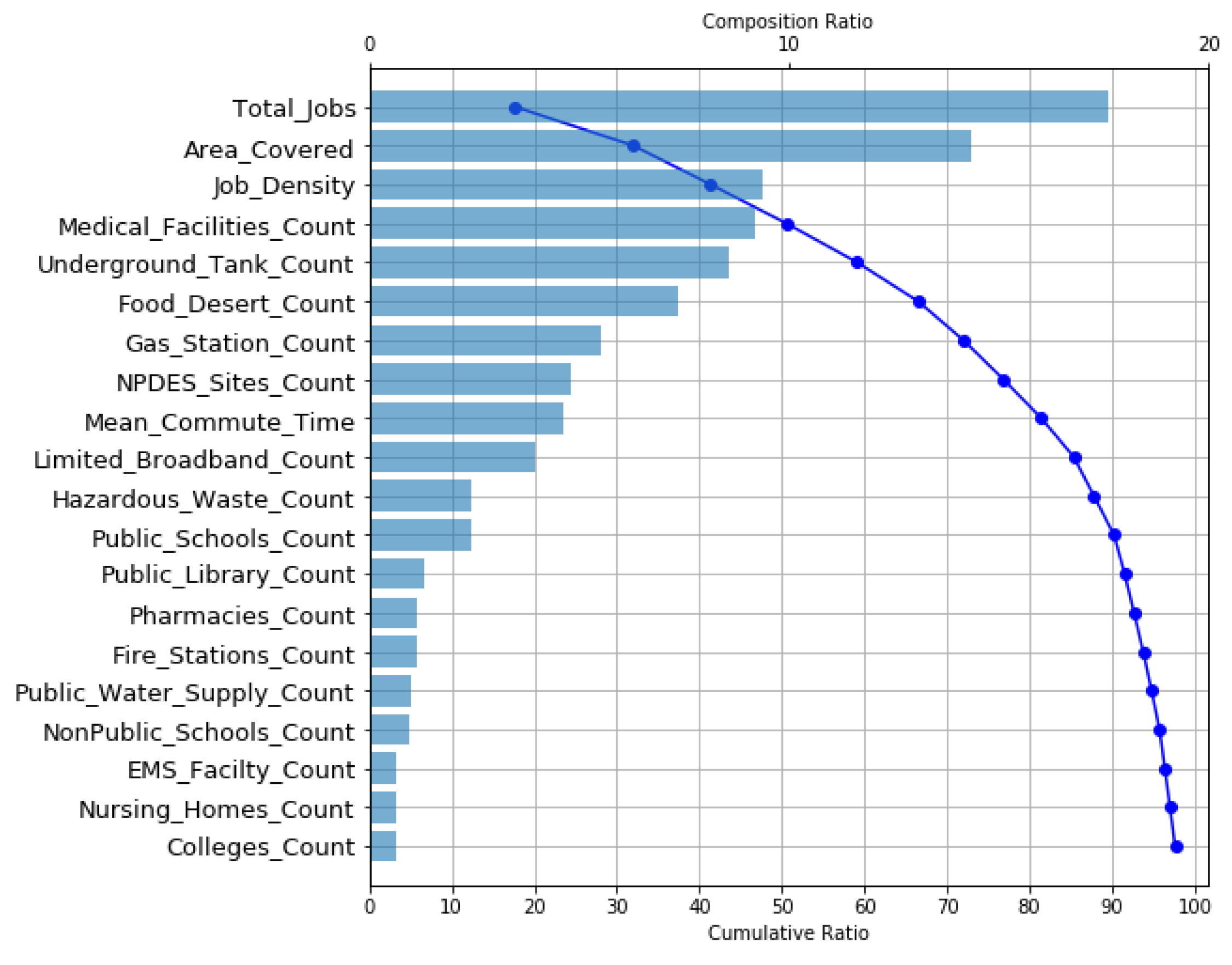
The impact of input variables on the prediction of RF model for spatial (in) justice is further explored with SHAP tool. The global importance factor of the input variables is illustrated in Figure 4. The global importance is estimated as the average of absolute Shapley values per feature across the data. The input variables are ranked in terms of importance, i.e., the higher the mean SHAP value, the more important the feature variable. As reflected in Figure 4, features such as “Total jobs”, “Area covered”, “Job Density”, “Underground Tank Count”, and “Medical Facilities Count” appeared to be the top five influential features in classifying spatially just vs. unjust places. The waterfall plot (blue line in Figure 4) also reveals that the number of total available jobs in a geographic location is the most important feature in the model, providing about 17% of the model’s interpretability, followed by the area covered by a geographic location, providing 14% of the model’s interpretability. The plot also suggests that the top 10 features provide about 85% of the model’s interpretation. It is also interesting to note that among the top ten most important features, four are from the “Economic Opportunity” category, three are from the “Basic Services” category, two are from the “Healthy Environment” category, and one is from the “Public Goods” category, as per Rocco’s characterization of Spatial Justice, depicted in Table 1. These results suggest that the model was able to learn features from most categories characterizing spatial justice and therefore has a potential to be effective in measuring spatial justice while being transparent and reliable.
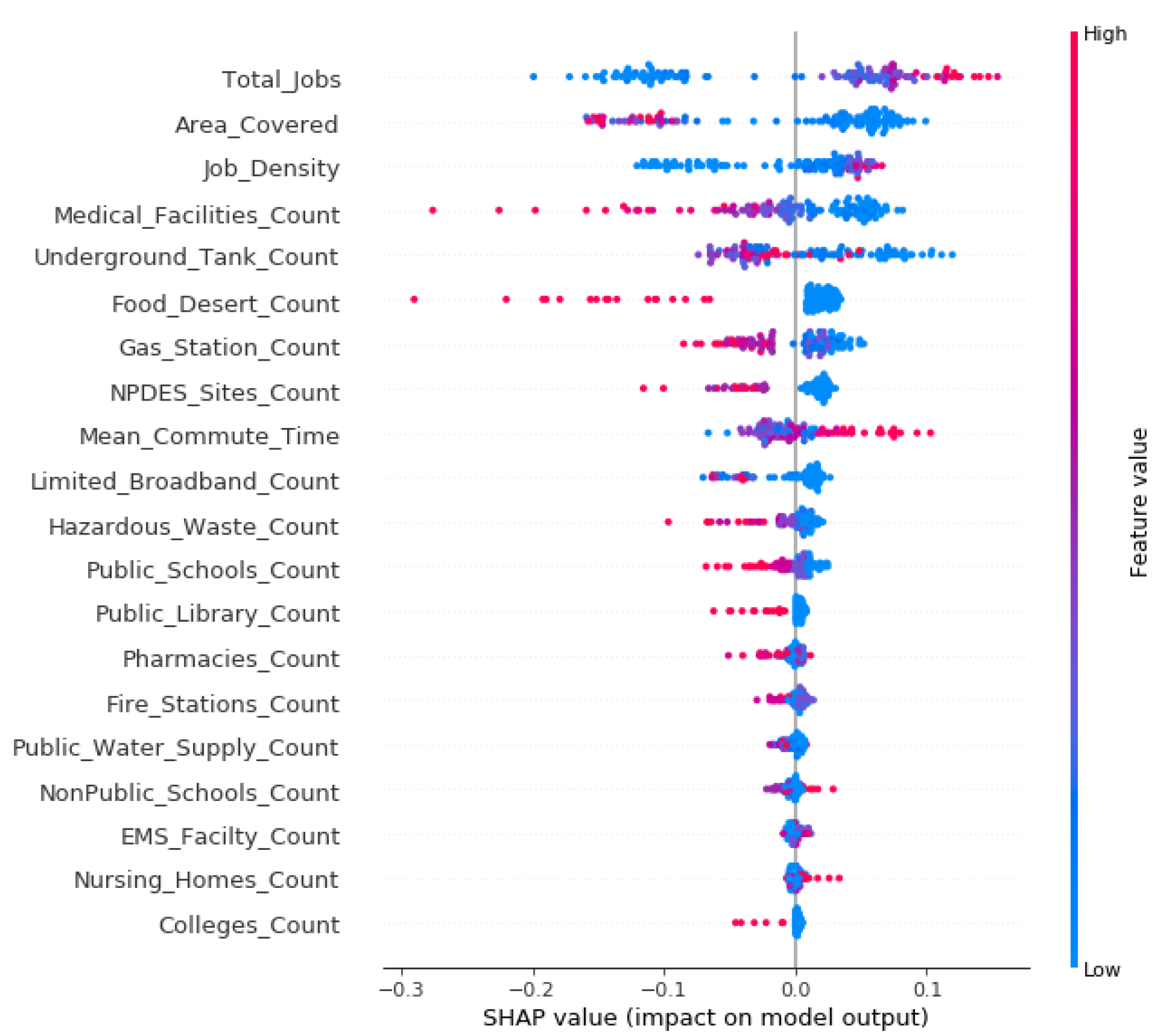
The range and distribution of impacts of input features on upward mobility predictions are also revealed through summary plots (Figure 5) via SHAP tool. Each point on the plots in Figure 5 is a Shapley value for the input variables and an instance. The y-axis indicates the input variables in order of importance from top to bottom. Each dot is colored by the value of the input variable, from low (blue) to high (red). The density of dots represents the distribution of points in the data set, i.e., whether it contains a range of values or selected ranges. Figure 5 shows that the higher values of the features “Total Jobs” and “Job Density” increase their SHAP values, and therefore push the prediction toward upward mobility (positive), on the other hand, the higher values of “Area Covered” pushes the prediction toward downward mobility (negative). These results could be interpreted such as an increase in total number of jobs at a certain census tract could potentially make it a spatially just place, on the other hand, a smaller and compact place tends to be spatially just. Similarly, an increase in “Medical Facilities Count”, “Food Desert Count”, “Gas Station Count”, and “NPDES Site Count” at a particular geographical location potentially could make the place unjust, whereas lower numbers of these spatial facilities favor spatially just places. A decrease in the number of “Underground Tank Count” certainly favors upward mobility and therefore spatially just places; on the other hand, an increase in “Mean Commute Time” enhances spatial justice.
6. Discussion
The results presented in Section 5.2 shed some lights on the questions a, b, and c that were posed in Section 4.2. These results suggest that the number and density of jobs available at a particular location, area covered by that location, number of available medical facilities, and the existence and frequency of underground storage tanks storing either petroleum or certain hazardous substances are most influential in determining economic mobility and in turn spatial justice of that location (answer to question: (a)). The next set of influential features are the existence and frequency of food deserts (an urban area in which it is difficult to buy affordable or healthy fresh food), gas stations, and NPDES (National Pollutant Discharge Elimination System) sites; limited broadband facility; and the amount of time needed to commute to workplaces.
The results of the SHAP analysis and corresponding plots also suggest that a spatially just area tend to have higher number of available jobs, compact form, lower number of facilities such as medical and gas stations, as well as absence or lower number of hazardous spatial features such as food deserts, underground storage tanks, NPDES sites, and limited broadband (answer to question: (b)). It is interesting to note that the model also suggests that the places with maximum commute time to work are spatially just places, meaning the suburbs and locations farther away from the city center are just places for the residents.
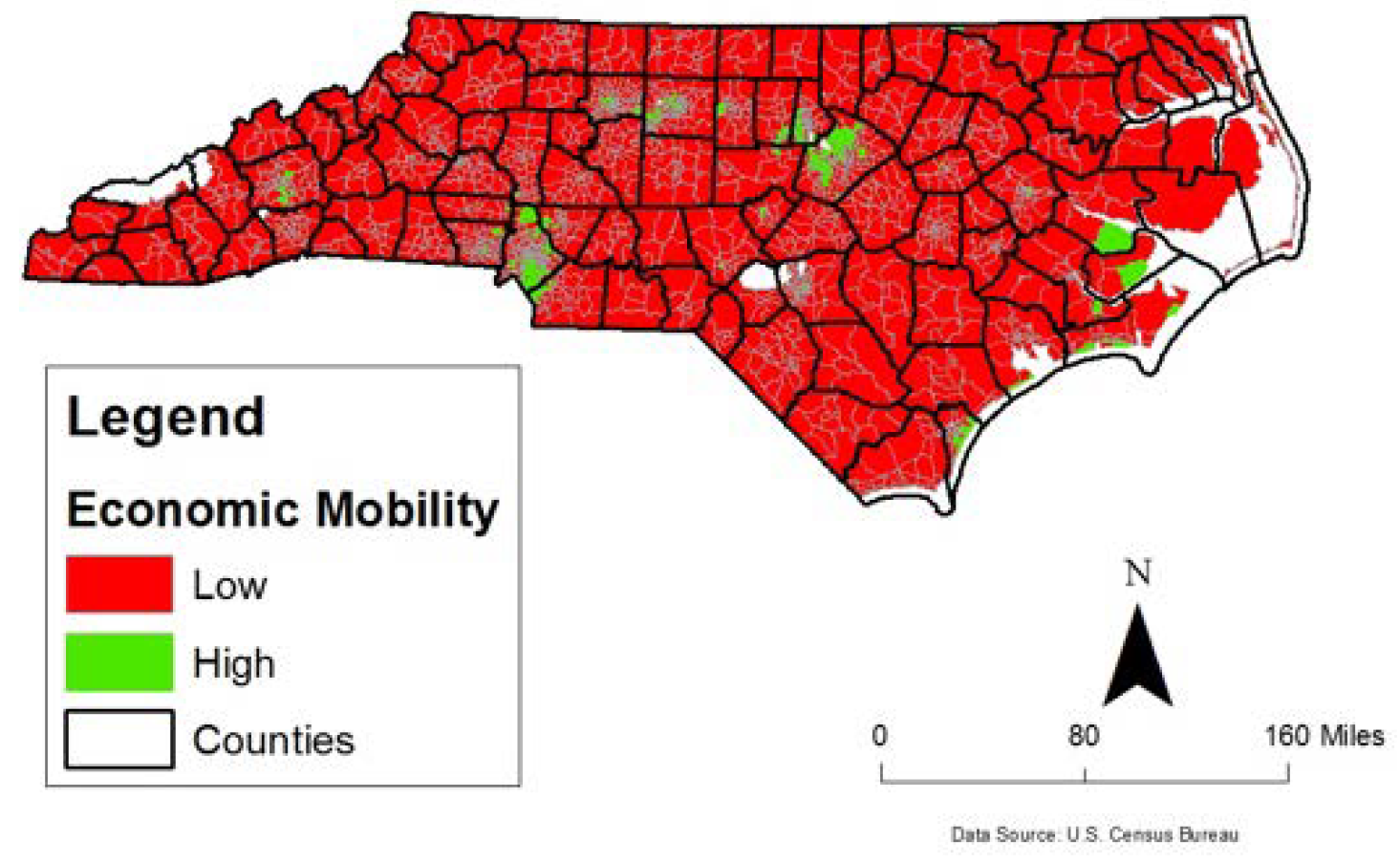
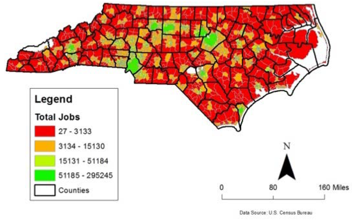
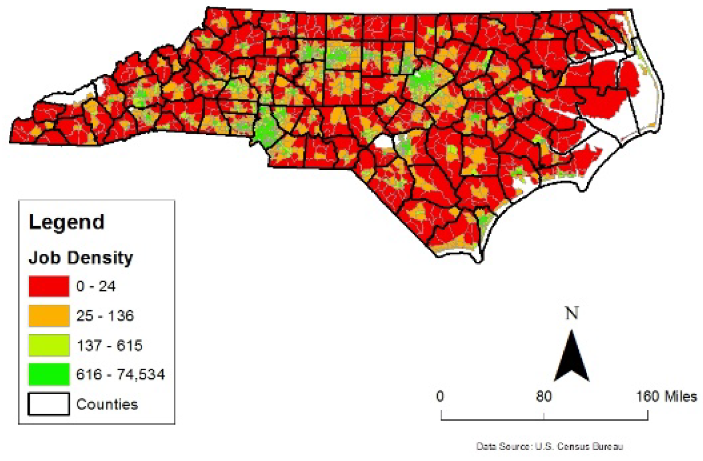
Similarly, a spatially unjust place tends to have the opposite characteristics in terms of the existence and frequency of the concerned features (answer to question: (c)). These results show that it is possible to measure spatial justice in terms of place-based factors and urban designers and policy makers can potentially include this to assess spatial (in)equality that a decision such as constructing a medical facility or manufacturing site (where many can be employed) at a particular geographic area could generate. Figure 6 highlights the level of economic mobility within each census tract and generally showcases the locations of NC’s urban centers. Not surprisingly, Figure 7 and Figure 8 clearly illustrate a positive relationship between these two employment related factors and the level of economic mobility as highlighted by the clusters of green census tracts that have both high economic mobility, large numbers of jobs, and high density of jobs. Meanwhile, Figure 9 shows the importance of compactness of the census tract. Smaller census tracts contain a high density of people and is thus generally related to better overall economic opportunities compared with geographically larger census tracts found in more rural spaces.
7. Conclusions
Through the application of data science and machine learning techniques, this study provides a way of characterizing spatial justice, and empirically evaluating the impact of spatial factors on economic mobility and in turn spatial justices. To the best of the authors’ knowledge, no studies were conducted to (1) explain the machine learning-based predictions of spatial (in)justice and (2) identify and rank the significant variables affecting spatial (in)justice. This article addresses these research limitations by (1) effectively characterizing spatial justice by a set of attainable public goods, basic services, cultural goods, economic opportunity, and healthy environments factors within a specific geographic area; (2) using RF to automatically predict spatially just vs. unjust places based on the chosen array of place-based variables; and (3) understanding the importance and contribution of spatial features for a specific prediction and visually interpreting the complex non-linear behavior of the underlying model through the use of SHAP. The comparative performance analysis of three classification algorithms reveals the superiority of RF model in predicting spatially just vs. unjust places based on spatial variables with 86% testing accuracy. The model is then explored with SHAP to identify the feature importance and decode the complex underlying relationships between spatial justice and input variables. The availability of jobs, compactness of the area, and the presence of facilities and hazardous sites have the greatest influence, whereas some of the influential features are positively while the others are negatively associated. In future, the capability of these predictive models will be tested on a national-scale data set.
Author Contributions
Conceptualization, Russell M. Smith; methodology, Russell M. Smith, Debzani Deb; software, Debzani Deb; validation, Debzani Deb; investigation, Russell M. Smith; data curation, Debzani Deb; writing—original draft preparation, Russell M. Smith, Debzani Deb; writing—review and editing, Russell M. Smith, Debzani Deb; visualization, Debzani Deb; funding acquisition, Debzani Deb. Both authors have read and agreed to the published version of the manuscript.
Funding
We would like to acknowledge the support provided by FY21-23 UNC Research Opportunities Initiative (ROI) award and NSF Award #1600864.
Institutional Review Board Statement
Not applicable.
Informed Consent Statement
Not applicable.
Data Availability Statement
Publicly available datasets were analyzed in this study. This data can be found here: https://www.nconemap.gov/, https://opportunityinsights.org/.
Conflicts of Interest
The authors declare no conflict of interest.
References
- Soja, E.W. Seeking Spatial Justice; Globalization and community series; University of Minnesota Press: Minneapolis, MN, USA, 2010; ISBN 978-0-8166-6667-6. [Google Scholar]
- Rocco, R.C. Why Discuss Spatial Justice in Urbanism Studies. Atlantis 2014, 24, 14–16. [Google Scholar]
- Fainstein, S.S. The Just City. Int. J. Urban Sci. 2014, 18, 1–18. [Google Scholar] [CrossRef]
- Williams, J. Spatial Justice as Analytic Framework. Ph.D. Thesis, University of Michigan, Ann Arbor, MN, USA, 2018. [Google Scholar]
- Wei, Y.D.; Xiao, W.; Simon, C.A.; Liu, B.; Ni, Y. Neighborhood, Race and Educational Inequality. Cities 2018, 73, 1–13. [Google Scholar] [CrossRef]
- Jones, A.; Mamudu, H.M.; Squires, G.D. Mortgage Possessions, Spatial Inequality, and Obesity in Large US Metropolitan Areas. Public Health 2020, 181, 86–93. [Google Scholar] [CrossRef] [PubMed]
- Rodríguez-Pose, A.; Storper, M. Housing, Urban Growth and Inequalities: The Limits to Deregulation and Upzoning in Reducing Economic and Spatial Inequality. Urban Stud. 2020, 57, 223–248. [Google Scholar] [CrossRef]
- Garcia, X.; Garcia-Sierra, M.; Domene, E. Spatial Inequality and Its Relationship with Local Food Environments: The Case of Barcelona. Appl. Geogr. 2020, 115, 102140. [Google Scholar] [CrossRef]
- Liu, C.; Duan, D. Spatial Inequality of Bus Transit Dependence on Urban Streets and Its Relationships with Socioeconomic Intensities: A Tale of Two Megacities in China. J. Transp. Geogr. 2020, 86, 102768. [Google Scholar] [CrossRef]
- Chang, Z.; Chen, J.; Li, W.; Li, X. Public Transportation and the Spatial Inequality of Urban Park Accessibility: New Evidence from Hong Kong. Transp. Res. Part D Transp. Environ. 2019, 76, 111–122. [Google Scholar] [CrossRef]
- Chetty, R.; Hendren, N.; Kline, P.; Saez, E.; Turner, N. Is the United States Still a Land of Opportunity? Recent Trends in Intergenerational Mobility; National Bureau of Economic Research: Cambridge, MA, USA, 2014; p. w19844. [Google Scholar]
- Bullard, R.D. Dumping in Dixie: Race, Class, and Environmental Quality, 3rd ed.; Westview Press: Boulder, CO, USA, 2000; ISBN 978-0-8133-6792-7. [Google Scholar]
- Weiher, G.R. The Fractured Metropolis: Political Fragmentation and Metropolitan Segregation; SUNY Series, the New Inequalities; State University of New York Press: Albany, NY, USA, 1991; ISBN 978-0-7914-0565-9. [Google Scholar]
- Orfield, M. Metropolitics: A Regional Agenda for Community and Stability; Brookings Institution Press: Washington, DC, USA; Lincoln Institute of Land Policy: Cambridge, MA, USA, 1997; ISBN 978-0-8157-6640-7. [Google Scholar]
- Deb, D.; Smith, R.M. Use of Machine Learning in Exploring Spatial (In) Justices 1. In Proceedings of the 2020 19th IEEE International Conference on Machine Learning and Applications (ICMLA), Miami, FL, USA, 14–17 December 2020; pp. 1211–1217. [Google Scholar]
- Breiman, L. Random Forests. Mach. Learn. 2001, 45, 5–32. [Google Scholar] [CrossRef] [Green Version]
- Miller, T. Explanation in Artificial Intelligence: Insights from the Social Sciences. arXiv 2018, arXiv:1706.07269. [Google Scholar] [CrossRef]
- Ribeiro, M.T.; Singh, S.; Guestrin, C. “Why Should I Trust You?”: Explaining the Predictions of Any Classifier. arXiv 2016, arXiv:1602.04938. [Google Scholar]
- Shrikumar, A.; Greenside, P.; Shcherbina, A.; Kundaje, A. Not Just a Black Box: Learning Important Features Through Propagating Activation Differences. arXiv 2017, arXiv:1605.01713. [Google Scholar]
- Lundberg, S.; Lee, S.-I. A Unified Approach to Interpreting Model Predictions. arXiv 2017, arXiv:1705.07874. [Google Scholar]
- Lundberg, S.M.; Erion, G.; Chen, H.; DeGrave, A.; Prutkin, J.M.; Nair, B.; Katz, R.; Himmelfarb, J.; Bansal, N.; Lee, S.-I. Explainable AI for Trees: From Local Explanations to Global Understanding. arXiv 2019, arXiv:1905.04610. [Google Scholar] [CrossRef]
- Lefebvre, H.; Deulceux, S.; Hess, R.; Weigand, G. Le Droit à La Ville; Economica-Anthropos: Paris, France, 2009; ISBN 978-2-7178-5708-5. [Google Scholar]
- Harvey, D. Geographies of justice and social transformation. In Social Justice and the City, Rev. ed.; University of Georgia Press: Athens, Greece, 2009; ISBN 978-0-8203-3403-5. [Google Scholar]
- Pirie, G.H. On Spatial Justice. Environ. Plan A 1983, 15, 465–473. [Google Scholar] [CrossRef]
- Fainstein, S.S. The Just City; Cornell University Press: Ithaca, NY, USA, 2010; ISBN 978-0-8014-7690-7. [Google Scholar]
- Chetty, R.; Hendren, N. The Impacts of Neighborhoods on Intergenerational Mobility I: Childhood Exposure Effects. Q. J. Econ. 2018, 133, 1107–1162. [Google Scholar] [CrossRef]
- Ewing, R.; Hamidi, S.; Grace, J.B.; Wei, Y.D. Does Urban Sprawl Hold down Upward Mobility? Landsc. Urban Plan. 2016, 148, 80–88. [Google Scholar] [CrossRef] [Green Version]
- Altzinger, W.; Cuaresma, J.C.; Rumplmaier, B.; Sauer, P.; Schneebaum, A. Education and Social Mobility in Europe: Levelling the Playing Field for Europe’s Children and Fuelling Its Economy; WWW for Europe: Vienna, Austria, 2015. [Google Scholar]
- Corak, M. Income Inequality, Equality of Opportunity, and Intergenerational Mobility. J. Econ. Perspect. 2013, 27, 79–102. [Google Scholar] [CrossRef] [Green Version]
- Black, S.; Devereux, P. Recent Developments in Intergenerational Mobility; National Bureau of Economic Research: Cambridge, MA, USA, 2010; p. w15889. [Google Scholar]
- Hardaway, C.R.; McLoyd, V.C. Escaping Poverty and Securing Middle Class Status: How Race and Socioeconomic Status Shape Mobility Prospects for African Americans During the Transition to Adulthood. J. Youth Adolesc. 2009, 38, 242–256. [Google Scholar] [CrossRef]
- Delgado, R. The Myth of Upward Mobility. Lawreview 2007, 68. [Google Scholar] [CrossRef] [Green Version]
- Powell, W.S. Encyclopedia of North Carolina; University of North Carolina Press: Chapel Hill, NC, USA, 2006. [Google Scholar]
- NC OneMap Geospatial Portal; North Carolina Government Data Analytics Center: Raleigh, NC, USA, 2020.
- Barandela, R.; Valdovinos, R.M.; Sánchez, J.S.; Ferri, F.J. The Imbalanced Training Sample Problem: Under or over Sampling? In Structural, Syntactic, and Statistical Pattern Recognition; Fred, A., Caelli, T.M., Duin, R.P.W., Campilho, A.C., de Ridder, D., Eds.; Lecture Notes in Computer Science; Springer: Berlin/Heidelberg, Germany, 2004; Volume 3138, pp. 806–814. ISBN 978-3-540-22570-6. [Google Scholar]
- Chawla, N.V.; Bowyer, K.W.; Hall, L.O.; Kegelmeyer, W.P. SMOTE: Synthetic Minority Over-Sampling Technique. JAIR 2002, 16, 321–357. [Google Scholar] [CrossRef]
- Bao, L.; Juan, C.; Li, J.; Zhang, Y. Boosted Near-Miss Under-Sampling on SVM Ensembles for Concept Detection in Large-Scale Imbalanced Datasets. Neurocomputing 2016, 172, 198–206. [Google Scholar] [CrossRef]
- Haibo, H.; Yang, B.; Garcia, E.A.; Li, S. ADASYN: Adaptive Synthetic Sampling Approach for Imbalanced Learning. In Proceedings of the 2008 IEEE International Joint Conference on Neural Networks (IEEE World Congress on Computational Intelligence), Hong Kong, China, 1–8 June 2008; pp. 1322–1328. [Google Scholar]
- Prusa, J.; Khoshgoftaar, T.M.; Dittman, D.J.; Napolitano, A. Using Random Undersampling to Alleviate Class Imbalance on Tweet Sentiment Data. In Proceedings of the 2015 IEEE International Conference on Information Reuse and Integration, San Francisco, CA, USA, 13–15 August 2015; pp. 197–202. [Google Scholar]
- Guyon, I.; Elisseeff, A. An Introduction to Variable and Feature Selection. J. Mach. Learn. Res. 2003, 3, 1157–1182. [Google Scholar]
Figure 1.
North Carolina counties and census tracts.

Figure 2.
Correlation matrix of all features.

Figure 3.
ROC/AUC values for each classifier.

Figure 4.
SHAP Waterfall plot illustrating most important features.

Figure 5.
SHAP Summary plot illustrating range and distribution of impacts of input features.

Figure 6.
NC census tracts by level of economic mobility.

Figure 7.
NC census tracts by total jobs.

Figure 8.
NC census tracts by job density.

Figure 9.
NC census tracts by compactness.


Table 1.
Identified spatial feature variables based on Rocco’s factors (28).
| Rocco’s Factors | Spatial Feature Variables |
|---|---|
| Public Goods (10) | Number of Schools |
| Water Service | |
| Sewer Service | |
| Fire Stations | |
| Hospitals | |
| Medical Facilities | |
| Correctional Facilities | |
| Emergency Medical Facilities | |
| Law Enforcement Locations | |
| Public Health Department | |
| Basic Services (5) | Gas Stations |
| Food Desert | |
| Limited Broadband | |
| Pharmacies | |
| Nursing Homes | |
| Cultural Goods (3) | Libraries |
| Colleges | |
| Non-Public Schools | |
| Economic Opportunity (4) | Mean Travel Time to Work |
| Total Jobs | |
| Jobs Density | |
| Area covered. | |
| Healthy Environment (6) | Underground storage tanks |
| Brownfields | |
| NPDES Sites | |
| Hazardous Waste Facilities | |
| Landfills | |
| Gamelands |
Table 2.
Classification accuracies on test data.
| Classification Algorithms | Precision | Recall | Accuracy | F1 | ROC |
|---|---|---|---|---|---|
| k-nearest neighbor (kNN) | 0.77 | 0.82 | 0.78 | 0.79 | 0.78 |
| Support vector machine (SVM) | 0.81 | 0.77 | 0.79 | 0.79 | 0.79 |
| Random forest (RF) | 0.86 | 0.85 | 0.86 | 0.86 | 0.86 |
Publisher’s Note: MDPI stays neutral with regard to jurisdictional claims in published maps and institutional affiliations. |
© 2021 by the authors. Licensee MDPI, Basel, Switzerland. This article is an open access article distributed under the terms and conditions of the Creative Commons Attribution (CC BY) license (https://creativecommons.org/licenses/by/4.0/).
Share and Cite
MDPI and ACS Style
Deb, D.; Smith, R.M. Application of Random Forest and SHAP Tree Explainer in Exploring Spatial (In)Justice to Aid Urban Planning. ISPRS Int. J. Geo-Inf. 2021, 10, 629. https://0-doi-org.brum.beds.ac.uk/10.3390/ijgi10090629
AMA Style
Deb D, Smith RM. Application of Random Forest and SHAP Tree Explainer in Exploring Spatial (In)Justice to Aid Urban Planning. ISPRS International Journal of Geo-Information. 2021; 10(9):629. https://0-doi-org.brum.beds.ac.uk/10.3390/ijgi10090629
Chicago/Turabian StyleDeb, Debzani, and Russell M. Smith. 2021. "Application of Random Forest and SHAP Tree Explainer in Exploring Spatial (In)Justice to Aid Urban Planning" ISPRS International Journal of Geo-Information 10, no. 9: 629. https://0-doi-org.brum.beds.ac.uk/10.3390/ijgi10090629
Note that from the first issue of 2016, this journal uses article numbers instead of page numbers. See further details here.