
Digital Soil Mapping of Soil Organic Matter with Deep Learning Algorithms


1
School of Cyber Science and Engineering, Zhengzhou University, Zhengzhou 450001, China
2
School of Water conservancy Science and Engineering, Zhengzhou University, Zhengzhou 450001, China
3
School of Civil Engineering, Zhengzhou University, Zhengzhou 450001, China
*
Author to whom correspondence should be addressed.
ISPRS Int. J. Geo-Inf. 2022, 11(5), 299; https://0-doi-org.brum.beds.ac.uk/10.3390/ijgi11050299
Submission received: 28 February 2022
/
Revised: 29 April 2022
/
Accepted: 2 May 2022
/
Published: 6 May 2022
Abstract
:Digital soil mapping has emerged as a new method to describe the spatial distribution of soils economically and efficiently. In this study, a lightweight soil organic matter (SOM) mapping method based on a deep residual network, which we call LSM-ResNet, is proposed to make accurate predictions with background covariates. ResNet not only integrates spatial background information around the observed environmental covariates, but also reduces problems such as information loss, which undermines the integrity of information and reduces prediction uncertainty. To train the model, rectified linear units, mean squared error, and adaptive momentum estimation were used as the activation function, loss/cost function, and optimizer, respectively. The method was tested with Landsat5, the meteorological data from WorldClim, and the 1602 sampling points set from Xinxiang, China. The performance of the proposed LSM-ResNet was compared to a traditional machine learning algorithm, the random forest (RF) algorithm, and a training set (80%) and a test set (20%) were created to test both models. The results showed that the LSM-ResNet (RMSE = 6.40, R2 = 0.51) model outperformed the RF model in both the roots mean square error (RMSE) and coefficient of determination (R2), and the training accuracy was significantly improved compared to RF (RMSE = 6.81, R2 = 0.46). The trained LSM-ResNet model was used for SOM prediction in Xinxiang, a district of plain terrain in China. The prediction maps can be deemed an accurate reflection of the spatial variability of the SOM distribution.
1. Introduction
Soil is the living skin of the earth, and it is the vehicle that sustains human activity and the growth of plants and animals [1]. The accurate understanding and rational interpretation of soil properties and spatial distribution patterns are the basis for the sustainable development of soil resources. Precise mapping of soil properties is in urgent demand in fields such as precision agriculture [2,3], land use planning [4], and environment protection [5]. Digital soil mapping (DSM) is an emerging, efficient mapping method widely used to predict soil classes and properties [6,7].
DSM reflects the patterns and characteristics of soil formation and development processes, using spatial analysis and mathematical methods as a technical means of predicting soil properties and mapping methods. In most cases, soil sample points are obtained using field collection, which is the main source of information on the spatial autocorrelation of soil properties and knowledge of the relationship between soil and environmental variables [1]. The current common method of soil mapping based on the collection of sample points utilizes the relationship between soil properties and environmental covariates for quantitative mapping. The formalization of the DSM methodology was completed by the publication of McBratney et al. [8]. Following Dokuchaev [9] and Jenny [10], they modeled scorpan as the empirical quantitative relationship between a soil attribute and its spatially implied forming factors [11]. The relationship between soil attribute data and geographic environmental data where the soil undergoes related or synergistic changes is often used to predict the spatial distribution of soil. Such methods draw on linear regression analysis or nonlinear regression analysis algorithms, which include artificial neural networks (ANN) [12,13,14], augmented regression tree models [15], and SVM [13]. Among these, random forest (RF) has become one of the most popular techniques in DSM prediction [16,17,18].
Researchers have found that, in predicting soil properties with the help of the scorpan paradigm, soil properties are not only related to the variations in environmental indices between the sampling points and the set of covariates represented by the points, but also the spatial information implied therein needs to be considered. Scientists have conducted experiments with methods that simultaneously consider environmental variables and spatial information at sampling points. A co-kriging interpolation method that builds on the theory of collaborative regionalized variables (spatial correlation) and uses the synergistic correlation between the target and environmental variables to create a cross-covariance function for local estimation of the target variables has been proposed [19]. Others uses regression kriging, where the residual terms of the regression kriging model are kriged to regionalized variables by regressing soil attributes on environmental variables, and finally added to the predicted values of the regression model to produce the final spatial distribution of soil attributes [20]. Geographically weighted regressions are local linear regressions that model nonparametric local spatial regressions based on the distance between sample points from the regression centroid and determine the weights of the model parameter estimates. The regression coefficients of the sample points in the model vary with spatial location, thus reflecting the spatial variation in the contribution of sample points and environmental variables to the regression equation [21,22,23]. However, these methods have certain requirements over the size and the distribution of the data, and modelling nonlinear relationships between soil properties or classes and numerous interrelated covariates is not concise, and therefore comes with additional challenges (e.g., too many parameters to be estimated) [24]. Challenges include if the samples do not meet the assumption of second-order smoothness, the model is computationally demanding, or requires a cumbersome data pre-processing process, which is often difficult to achieve in practical applications [25,26,27].
With the rapid development of big data, deep learning (DL) has proven to be a new tool of analysis in many fields. Unlike other physical models that rely heavily on prior knowledge of parameters, DL methods utilize feature representations derived from data alone [28]. These methods better represent nonlinear relationships, especially complex nonlinear relationships between different environmental attributes, through a large number of process features generated during model training, while having higher prediction accuracy compared to geostatistics and other traditional machine learning (ML) methods [29,30].
Convolutional neural networks (CNNs) [31] in deep learning have gained much attention, specifically as a multilayer interconnected neural network that has yielded good results in different computer vision domains. The algorithm discovers a distributed feature representation of the data by using a sliding window approach in combination with the underlying features to form a more abstract high-level feature representation. It uses the sliding window approach to extract local and spatially distributed features of environmental covariates from spatial sources and coordinated soil observations to make spatial estimates of soil properties [7]. Thus, CNNs resolve a rather major issue of machine learning (ML) methods because the networks use the spatial structure of the input, rather than just the covariate information of the sampled points, making better use of background covariate information, while the algorithm adds a large number of distributional features.
CNNs are mostly used for classification problems in computer vision and remote sensing studies, e.g., with the Land Use/Land Cover Area Framework Survey (LUCAS) dataset by Veres et al. [32], CNNs were used for soil spectral classification. Volpi et al. [33] used CNNs for land cover classification using high-resolution remote sensing imagery. While for spatial estimation of soil properties, the potential of deep learning in multi-scale terrain feature construction and its relative effectiveness in digital soil mapping was first outlined in the work of Behrens et al. [34]. Padarian et al. and Wadoux et al. proposed using CNNs to predict the content of SOC [11,35]. They report that CNNs have an advantage over standard ML algorithms in terms of prediction error. Tsakiridis et al. developed a new framework using a local multichannel 1D CNN to continuously estimate different soil properties (e.g., SOC) [36]. The CNNs architecture consistently outperformed RF models in predicting the soil particle size fraction (PSF) [37].
ResNet, as a branch architecture of CNNs, has received more attention in the past few years. The expressive power of deep neural networks and the ability to extract features increase with the depth of the network, but the model accuracy decreases rapidly when the number of network layers increases to a certain number [38,39]. To solve the problem of network degradation due to the increased depth, He et al. proposed the ResNet deep learning framework [40], which introduces the concept of constant mapping in the network and redefines each layer as a residual learning function due to input through the reference layer instead of learning the unreferenced function, thus simplifying the training of the network, increasing the number of information transfer paths, and greatly improving the system’s accuracy. Due to the good performance of ResNet, it has been applied to many fields of computer science, such as image recognition [41] and semantic segmentation [42]. Song et al. [43] designed a residual network for sea ice classification, called SI-ResNet, which achieved good classification accuracy. Zhang et al. [44] combined ResNet-V2 to design a small ResNet for remote sensing classification recognition, and the accuracy outperformed the classical classifier. ResNet is one of the most effective deep learning network frameworks for image detection and classification to date.
Based on the above analysis, deep learning methods are proposed to be used for DSM. This study proposes an innovative lightweight deep learning architecture (LSM-ResNet) based on ResNet, which implements an end-to-end process for SOM regression prediction using multiple sources of data. To train the network, we constructed a soil covariate dataset based on RGB images based on image fusion. The effect of pre-frame size on model error was analyzed. We selected SOM as a predicted soil attribute, which is an important indicator of soil quality index, soil fertility, and soil health. A detailed and high-quality SOM map can provide important basic data for ecosystem modeling and climate policy development [5,45,46,47,48]. Accurate information on spatial changes in SOM is useful for land use planning and other activities related to forestry, agriculture, environmental protection, and land degradation management [5]. The performance of the LSM-ResNet proposed in this study was compared with RF, as the RF algorithm is often used for DSM, and therefore is a logical comparison.
2. Methodology
2.1. Study Area
Xinxiang is located at the southwest of the North China Plain, approximately between 34°55′ N–35°50′ N and 113°30′ E–115°30′ E (Figure 1b), with an area of about 6434 km2 of plain, accounting for 77.36% of the total area of the region. It is dominated by a warm temperate continental monsoon climate with a mean annual temperature of 13–15 °C and an average annual precipitation of 573.4 mm. The Feng-huang Mountain area belongs to the northern hilly area. From NW to SE, the landforms transition from mountains to hills and then to plains. It is a transition zone between the alluvial plain of the Yellow River and the pre-mountain alluvial plain. The Haihe River and the Yellow River are the two main water systems. According to the Chinese Soil Taxonomy [49], there is a small amount of yellow sandy soil in the center, and brown soil and cinnamon soil are the two main soil types [50,51].
2.2. Soil Samples
The study utilized soil samples from the 2006 to 2008 cropland productivity evaluation project. The location, sampling depth, parent material, soil type, land use pattern, and other relevant information for each sample were recorded in detail.
All soil samples were air-dried and passed through a 0.25 mm sieve and then analyzed for SOM using the potassium dichromate volumetric method [52]. A total of 1602 soil samples were divided into three separate datasets, of which 80% were used to train and validate the model, and the rest were used for testing purposes.
2.3. Dataset and Pre-Processing
SOM content is controlled by multiple environmental and ecological factors and their interactions [5]. Based on a review of the literature [5,15,22,45,46,53], a set of 13 covariates representing climate, topography, and remote sensing were selected as potential predictor variables to predict SOM (Table 1). These variables were resampled to a spatial resolution of 30 m × 30 m, consistent with that of Landsat5 data. For each variable, its values were extracted in the 30 m × 30 m pixels where each soil sample was located. Four examples of selectable covariate data are shown in Figure 2.
In general, climatic factors determine the general pattern of SOM content [5,54]. Mean annual precipitation (MAP) is one of the most widely used climate factors in SOM predictions. To obtain the MAP, ArcGIS was used to derive the MAP based on information provided by WorldClim 2.1 [55], which were spatially resolved to 1 km and resampled to 30 m using the cubic interpolation method. Four topographic factors were derived from the Shuttle Radar Topography Mission (SRTM) digital elevation model (DEM) at a resolution of 30 m (https://gdex.cr.usgs.gov/gdex/ (accessed on 14 August 2021)), including elevation, slope, aspect (aspect is a circular measure that cannot be used directly in modelling, and therefore was converted to northness and eastness), and the topographic wetness index (TWI) [56].
For the RS data, we used five spectral bands from Landsat5 (https://gdex.cr.usgs.gov/gdex/ (accessed on 17 August 2021)), and three RS indices [2] as potential predictors. The five RS-based spectral bands and RS data were derived by filtering 38 Landsat5 images of Xinxiang City taken from June to August of each year (annual sampling time) from 2006 to 2008, and the average value was calculated.
Pre-processing of the RS data (e.g., radiometric correction and atmospheric correction) was done with ENVI 5.3. In our study, we used Landsat5 images to extract reflectance values of five bands: b1 (Band1, Blue), b2 (Band2, Green), b3 (Band3, Red), b4 (Band 4, NIR), and b5 (Band 5, SWIR). Remote sensing indices were also calculated using Landsat5 reflectance products: normalized difference vegetation index (NDVI) [57], enhanced vegetation index (EVI) [58], and difference vegetation index (DVI) [59]. The average of the three remotely sensed indices was calculated as a predictor.
Stepwise regression and correlation coefficient were used to select the most important environmental covariables to model SOM content. Finally, Landsat5 b4 (band 4, NIR), MAP, and NDVI consisting of RGB three-channel images (which is the number of image channels commonly used in computer vision) were selected to predict the SOM content of the study area. This is because these covariates have distinct feature expressions and a high correlation SOM. As image datasets, the selected covariates were normalized to a 30 m grid size by aggregation (mean resampling) or decomposition (bilinear resampling).
To allow for a fairer comparison between RF and LSM-ResNet, we used mean filters with different neighborhood sizes (radii of 1, 3, 5, 7, 9, 15, 21, 29, and 50 pixels) for effective multi-scale covariate information extraction [60]. This approach acts on night covariates: aspect (aspect to northness and eastness), MAP, slope, elevation, Landsat b4 (NIR), TWI, Landsat5 Band 5 (SWIR), and normalized vegetation index (NDVI), generating a total of (9 × 9) 81 new covariates as independent variables (using a bilinear approach to extract covariate data) to build the RF model. The mean filter is the most common method used in DSM studies for DEM multiscale mapping, and to filter the new covariates, the ANOVA method was used [18,60,61]. Figure 3 represents the methodology of the present study.
3. Deep Learning
Deep learning is a research method derived from artificial neural networks that can learn the representation of data through powerful multi-layer architectures. The residual network (ResNet) has achieved good results in many areas of imaging. Examples include face recognition, target detection, and semantic segmentation. ResNet and some related methods used in the model are introduced in this section.
3.1. ResNet
In this article, the context information we use is to represent the model’s covariates as a square format image around the soil measurements. Covariates may describe the distribution of SOM through a particular shape of the terrain or temperature and precipitation characteristics. With several alternative settings, the goal is to extract the most relevant features from the entire auxiliary dataset. In this case, CNNs are better to adapt than ANNs. ResNet is based on the deep residual network proposed by He et al. of Microsoft Research Asia in 2015 [40]. The core of ResNet is a residual block structure, as shown in Figure 4. It uses a shortcut connection called the cross-layer connection between input X and F(x) obtained through stacked weight layers, outputing . as the residual. The formula is as follows:
where F is the residual function, is the rectified linear units (ReLU) nonlinear activation function, and and are the weight layer. Assuming that Y is the output earth 4D feature matrix of the residual block, when the residual is connected with equal-dimensional mapping, as shown in Equation (2), X performs the convolution operation and the residual plus x gives Y.
If the dimensions of the two are different, then a linear mapping of the input x is needed to match the dimensions as shown in Equation (3).
where denotes the weight layer and denotes the linear mapping function.
Thus, the cross-layer connection of ResNet residual blocks is achieved by using the output of the previous layer directly as an input to the result of the next layer. After the cross-layer connection operation, it becomes learning and optimization of the residuals . In this way, the gradient does not disappear as the depth of the network increases and always maintains a significant variation in the backpropagation process, facilitating the optimization. Thus, the network can achieve better results.
3.2. Data Augmentation
In addition to the dropout layer, data augmentation techniques are used to further avoid overfitting and improve the universality of the model. Data augmentation [31] is a process that uses several random transformations to generate more training samples from the existing training data. It is known that there are many ways of data enhancement, and soil covariate features as pixel-level features can change the information of the images themselves if they are enhanced by panning, stretching, etc. This experiment rotates the existing training data by 90°, 180°, and 270° to increase the number of training samples. The main purpose is to allow the model to explore more aspects of the training samples and thus improve the universality ability of the network.
3.3. Using Soil Sample Data for Modelling in ResNet
In classification or regression prediction in computer vision, ResNet uses image classification datasets for annotation, modeling, and analysis. Most of the datasets in the computer vision domain are used for classification or regression of one object or several classes of objects in a single image. In this experiment, we use the whole image as a learning sample. The RGB three-channel image dataset is generated by combining multiple covariates (e.g., terrain attributes or climate data). Therefore, the spatial attribute information of covariates is no longer considered by pre-processing, for example, by multi-scale fusion of covariate data. Rather, soil sample data are used directly in ResNet, making direct use of spatial contextual information through a background or patch-based approach. These images are then equivalent to the common input images. For each sample, the square area around the sample is cropped out of the covariate dataset. These images are used as input images for ResNet. However, in addition to the usual ResNet hyperparameters, this requires optimizing the size of the patches.
3.4. Model Definition
In this study, we constructed a deep neural network structure called LSM-ResNet for predicting SOM content by fusing NDVI, band 4(NIR), and MAP data. The SOM covariate dataset was randomly assigned between the training and validation set (80%) and the test set (20%). All soil measurements were normalized between 0 and 1 using the minimum and maximum values of the calibration set. In addition, all covariates were centered and scaled with mean of 0 and standard deviation of 1. The structure is based on AlexNet [31] and ResNet [40], with modifications and tuning of the original network to allow for a small number of categories in the dataset images as input data. In the field of machine learning, different patch sizes of inputs can have an impact on the regression results. It is important to explore the impact of different patch sizes on performance based on LSM-ResNet. For the evaluation of models, the root mean squared error (RMSE), mean absolute error (MAE), and coefficient of determination (R2) are commonly used. To further evaluate the LSM-ResNet regression results, the LSM-ResNet was also compared with those obtained using the random forest (RF) model. The details of LSM-ResNet structure, parameter estimation, and evaluation functions commonly used in regression analysis are presented in Section 3.4.1, Section 3.4.2 and Section 3.4.3, respectively.
3.4.1. LSM-ResNet for SOM Mapping
Neural networks can establish intrinsic connections between input–target pairs when they are well correlated [62]. The architecture consists of two parts: the first part is convolutional filtering for hierarchical feature extraction, and the second part is a fully connected layer, consisting of layers of fully connected neurons with multiple input values. The convolutional layer (Conv) acts as a feature extractor by convolving with the input data, usually using multiple kernels of a specific size. The convolved features are then nonlinearized by the activation layer to produce a feature mapping. The pooling layer compresses the feature mappings to reduce redundancy and converts the output to vectors in a final pooling process. The fully connected (Fc) layer combines all the features learned in the previous layer to determine the desired pattern.
Deep learning models have been widely used in image regression [11,37,63,64]. Among different models, deep residual neural network models, especially ResNet models, can solve the problem of gradient explosion and gradient disappearance by using the “shortcut connection” method of cross-layer connection. Therefore, based on the characteristics of Landsat TM images and the principle of the ResNet model, we designed a lightweight pixel-based deep residual neural network model, the LSM-ResNet, to predict SOM content (Figure 5), and the detailed configuration is shown in Table 2.
The LSM-ResNet model starts with a set of convolutional layers with filter sizes of 3 × 3 and 3 × 3, where the ReLU activation function is used [65]. They are used to obtain the large neighborhood features of the model and image denoising. The convolutional layers are followed by a lower sample feature mapping layer with a maximum pool size of 2 × 2 (e.g., reducing the height and width of the features) and a dropout layer, while disconnecting the randomly connected half to prevent overfitting [66,67]. Two residual modules are then used, each of which is initially divided into the main path and a shortcut. The main path has two convolutional layers to extract deep features of the soil feature map, while the shortcut has only one convolutional layer to facilitate the upward propagation of residuals during training. The features obtained by the main path and the shortcut are reconstructed at the end of the residual module. As mentioned above, the blocks in the LSM-ResNet model are shown in Figure 5b. Each block consists of three layers: a weight layer (parameters of the convolution), a ReLU activation layer, and a batch normalization (BN) layer. BN on top of the residual blocks themselves prevents gradients from disappearing and exploding in each residual block, which can effectively improve the training efficiency. Afterward, using Global Average Pooling instead of flattening can minimize the number of parameters. The architecture used in this paper has three fully connected layers that receive information and produce predictions based on the previous layer.
To compare the prediction results of LSM-ResNet and the reference method, we also calibrated the RF model. Machine learning in DSM is well known for its excellent performance, and RF outperforms multiple linear regression and even other machine learning techniques in most studies [66,67,68,69]. In this experiment, a Bayesian optimization procedure regulating the optimal number of decision trees (n_estimators) and the number of input covariates in each random subset (m_estimators) was designed for RF-based SOM prediction. The n_estimators values ranged from 50 to 1000, and the number of different subsets ranged from 2 to 30. Based on Bayesian optimization, the number of decision trees was eventually determined to 700, and the number of input covariates was set to 5. According to the RandomForestRegressor function in the scikit-learn library, the other parameters in the RF were left as default values. To make fair comparisons among several models, we used the same calibration and test set with standardized SOM measurements and standardized covariates as inputs.
3.4.2. Parameter Estimation
Once the LSM-ResNet model is determined, the minimum MSE is used as the objective function to estimate the parameters, and an Adaptive Momentum Estimation (Adam) optimizer is used for this experiment. The model was trained with different window sizes of input images. We compared models of input covariable pixels with window sizes of 3, 5, 7, 9, 15, 21, 29, and 50. The comparison was based on the average RMSE on the validation set. The proposed network was implemented in Python using the Keras package version 2.1.0 [68] and Google’s TensorFlow library [69]. Once the input window size was selected, Bayesian optimization was applied to optimize the hyperparameters of the model architecture [70]. Bayesian optimization finds optimal values for machine learning hyperparameters in fewer iterations than random search. In this work, we optimized the filter number, the number of neurons, the batch size, and the learning rate using 63 iterations.
3.4.3. Validation Indices
Five common indices, namely the root mean squared error (RMSE), mean absolute error (MAE), Lin’s concordance correlation coefficient (CCC), mean error (ME), and coefficient of determination (R2) were used for validation. RMSE indicates the accuracy of the model prediction. MAE is a measure of model accuracy, but it is less sensitive to outliers than RMSE. R2 varies between 0 and 1 and indicates the closeness of the predicted values to the fitted regression line between predicted and observed values or the proportion of variance explained by the independent predictors. The bias is assessed by the mean error (ME).
where and are the predicted and actual values of the validation sample points, respectively, and is the actual value of the mean value.
CCC [71] is a reliability measure based on covariance and correspondence, with the Lin’s correlation line through the origin, assessing the agreement between measured and predicted values for a 1:1 line with a slope of 1.0.
where and are mean and variance for either the vector of true measurements or the vector of predicted values , respectively. The value represents the correlation between and .
4. Results
Figure 6 shows the RMSE of the SOM for different peripheral dimensions of the input image for the LSM-ResNet model. The background information is considered by representing the input data as a square format image around the soil measurement point. Each pixel has a resolution of 30 m × 30 m, so a window size of 3 × 3 pixels contains the contextual information of approximately 45 m. When using a window size of 5 × 5 pixels, the RMSE becomes significantly smaller. The lowest average RMSE is found with a window size of 15 × 15 pixels (contextual information of about 245 m). The data show that the model calibration does not benefit from using larger window sizes, as the RMSE values are increasing for window sizes of 29 × 29 pixels and 50 × 50 pixels. When using the LSM-ResNet for prediction, the model does not allow for the use of multiple input window sizes, so all the results presented later use an input window size of 15 × 15 pixels.
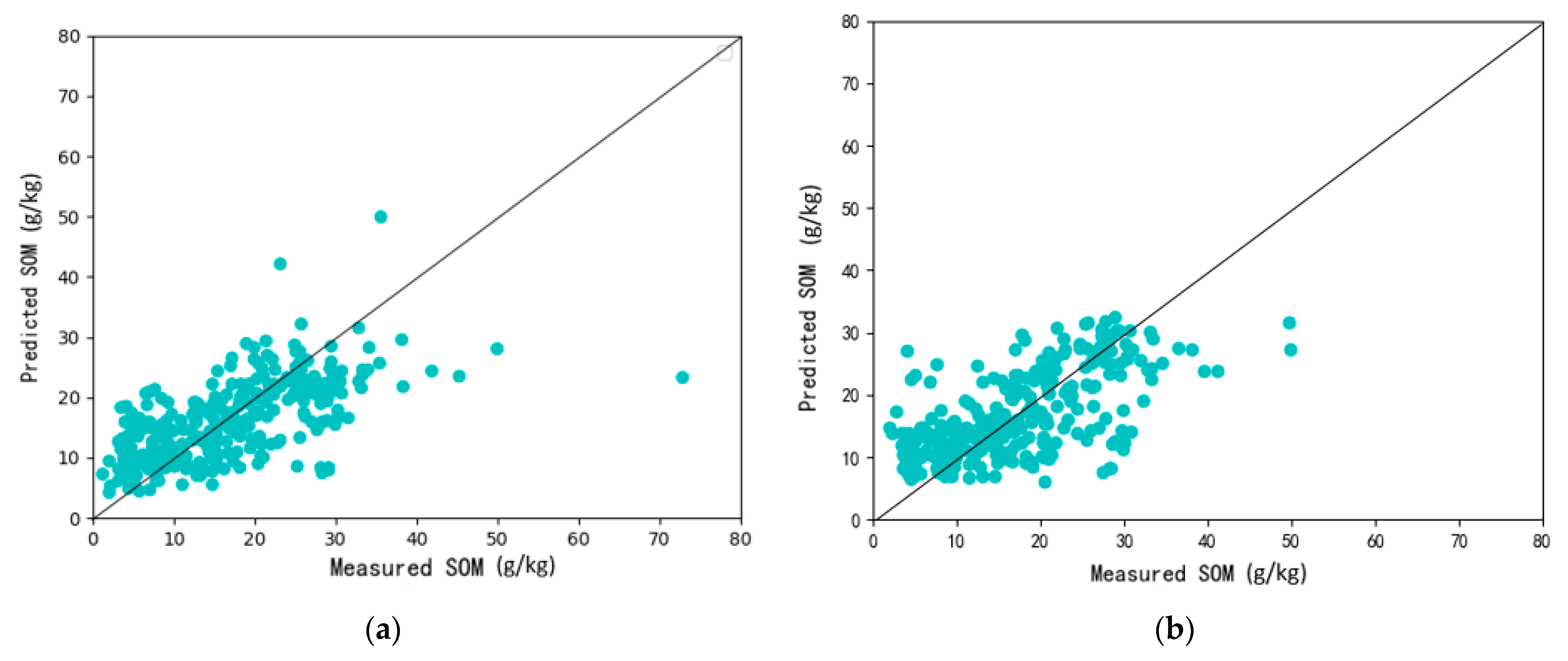
Figure 7a,b show the scatter plot of predicted and observed SOM values for the test data from the LSM-ResNet and RF models, respectively. Most predictions are collected on a 1:1 line. In general, both LSM-ResNet and RF models tend to overestimate SOM observations between 0 and 10 g/kg and underestimate SOM observations above 30 g/kg, with most observations concentrated between 10 g/kg and 30 g/kg. Compared to the LSM-ResNet, the predictions using RF were more scattered, with several overpredictions in the low range of the measured SOM values. The visual inspection in Figure 7 shows that the LSM-ResNet predicted more accurately than the RF.
To confirm this qualitative assessment, model performance metrics were generated (Table 3) and compared for both models. LSM-ResNet accuracy measures were on average equal to or better than RF. Based on RMSE and R2 values, LSM-ResNet (R2 = 0.51) outperformed RF (R2 = 0.46). CCC indicates that the reliability of LSM-ResNet (CCC = 0.71) based on covariates and correspondences is better than RF (CCC = 0.64). ME (in g/kg) showed that the predictions of both models are relatively unbiased. The LSM-ResNet model provides a small measure of accuracy (RMSE of 6.40 against 6.81 for the RF model) while providing a greater degree of prediction like falling on the 1:1 line past the origin.
Figure 8a,b shows the prediction plots of SOM based on LSM-ResNet and based on RF. The prediction results of the deep learning models are shown in a smooth but detailed plot. The prediction map gives a good indication of the spatial variation trend of surface SOM content. The high-value areas on the prediction map appear in the southeastern and central parts of the study area, and the prediction map accurately reflects the variation characteristics of SOM in the study area to a certain extent. From the Figure 8, it can be seen that the high-value and low-value areas in the study area are obvious and have obvious spatial distribution characteristics, the SOM map (Figure 8b) generated from the RF model was found to rely heavily on the MAP covariate, and as such, the spatial patterns of MAP are evident in the SOM map. The low-value zone (5–9 g/kg) appearing in the central part is well reflected in the LSM-ResNet (Figure 8a) prediction map, with obvious differences from the surrounding SOM content.
5. Discussion
5.1. Effect of the Input Window Size
The effect of the window size of the input image on the accuracy of the prediction is shown in Figure 6, and when using images with different window sizes, the optimal image size is 15 pixels, which corresponds to a contextual information of about 225 m for this study, and the RMSE for this image size is also the lowest. This suggests that the contextual information of the auxiliary data within 225 m is more useful for predicting SOM than the local information of a specific point where only a single soil property measurement is available. This is also the expected result reported by Padarian et al. [11]. The window size is closely related to the contextual information provided to the model. The model integrates the spatial context by considering the covariate pixels near the sampling locations. More additional background can improve the predictive power of the model, but too much background information will certainly generate noise. Padarian et al. [11] found an optimal range of window sizes in the case studies where topographic attributes were derived from the DEM used in the soil survey. However, it is worth noting that the optimal window size in DSM analysis varies from case study to case study depending on the spatial resolution of the input data and the characteristics of the landscape. Some authors have provided equivalent values of spatially relevant range for the SOM. Kumhalova et al. [72] reported values for the spatial correlation range of organic matter between 240 and 270 m using data from an experimental site in the Czech Republic. Similarly, Jian-Bing et al. [73] found a spatial correlation range of 309 m for a small watershed in northeastern China. For our study, we tested this hypothesis by fitting the spherical semi-variogram function to the experimental variogram of SOM. The fitted value for the range is 216 m, close to the window size we found. However, it is difficult to draw conclusions based on the predicted results. The relationship between the correlation range of the window size and the autocorrelation distance of the SOM needs to be further explored.
In our study, we found that a window size between 13 × 13 pixels and 18 × 18 pixels was optimal. DEM, as one of the important factors affecting SOM, was chosen by several other authors as a covariate to compose the RGB images [11,35]. However, in this experiment, the plain area occupied 78% of the total area. The topographic attributes of the plain area were less variated, and the expression of topographic attributes such as elevation was not obvious. It is known that the prediction of soil attributes in plain areas has been a difficult problem, and a good prediction accuracy was achieved in this experiment without selecting topographic attributes as covariates. Outside this range, the prediction accuracy may be 6% lower than the highest accuracy value. Therefore, it can be assumed that there is a spatial autocorrelation between a certain range of contextual information and the SOM of plain areas. However, further research is needed to draw general conclusions about the relationship between the range of autocorrelation of soil properties and window size [60]. Investigation of this issue would certainly make a valuable extension to future DSM studies.
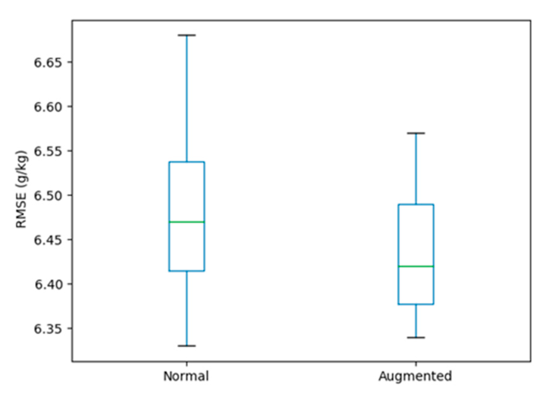
5.2. Data Augmentation
To generalize and improve the LSM-ResNet, we created new data by rotating the original image input and using only the information from the training data. The data augmentation was effective in reducing the model error (Figure 9), and a 3% reduction in model error was observed. Studies have generally shown that data “augmentation” can improve the accuracy of classification tasks [74]. It is assumed that by increasing the amount of training data, we can reduce the overfitting phenomenon of LSM-ResNet. In terms of data spatial autocorrelation, we need to consider that in the case of data augmentation, we have four sampling points at the same location with the same SOM content at the sampling points, so assuming that the distance is equal to 0 makes no difference if we consider the distance to be exactly equal to 0 [35]. However, it did not substantially reduce the error of the model (with and without data augmentation) [11,35]. Few people have discussed this, as covariate images have a different data representation than the images often used in computer vision. We tentatively assume that the data augmentation effect of covariate pictures is related to the selected covariates. DEM achieves better data enhancement than other covariates under the same conditions (e.g., weather and DEM), because DEM has more distinct spatial information features and performs better when mining shallow data features. However, it is undeniable that deep learning requires a large number of samples to train the model, and data augmentation can be very helpful for soil mapping based on deep learning [74].
5.3. Interpretation of the Map Features
In Figure 8a, we give the predicted SOM content map using the proposed LSM-ResNet architecture. The overall organic matter content interval ranged from 2 to 40 g/kg and was heavily concentrated in a 10–20 g/kg margin. The map shows that the SOM content of the study area decreases from northwest to southeast, with the edge of the Taihang Mountains in the northwest of the study area and the Yellow River in the south, and the topography changes from hills to plains as the elevation decreases. It is generally believed that SOM content is significantly and positively correlated with altitude, and the SOM content is higher in the relatively high altitude (18–25 g/kg of organic matter) in the northwest than in other plain areas. Meanwhile, we found obvious organic matter dividing lines at the edge of the Taihang Mountains, where organic matter was more accumulated at the bottom of the slope than on the ridge, and organic matter changes had obvious spatial variation. Xinxiang City is an important grain producing area in China, 78% of which is in the plain area, while the central area (19–27 g/kg of organic matter) has a large amount of farmland, and effective soil management measures have significantly increased the SOM content in the central area. The central low-value area is partly the ancient Yellow River basin, which is dominated by yellow sandy soils, which are known to have a much lower organic matter content than other soils. This is the reason why the central region has a low-value zone. Figure 8b shows the distribution of the SOM based on the random forest model after calibration. We noted a striped region in the middle of the southeast direction, which was not present in the prediction map of LSM-ResNet. We think the reason is that the region is a plain area, some covariates (e.g., DEM, Aspect) in RF prediction do not vary much, and the model is more influenced by a single covariate (MAP), while LSM-ResNet can utilize more depth features through deep learning and has better performance in the plain area.
By comparing Figure 8a and b, perhaps another advantage of the ResNet model is that it can make better use of covariates. This is shown by the fact that the predictions of the RF model show the spatial trend of MAP, while ResNet uses the same covariates but does not. Thus, perhaps this effect of ResNet in protecting DSM maps is common when using coordinates as predictors. A similar pattern of spatial variation is seen in the SOM predicted by both models, with a decreasing trend from northwest to southeast. As can be seen in the figure, the average map of the mapping using the LSM-ResNet architecture shows a smooth but detailed pattern with significant spatial variation.
5.4. Analyses of the Results of the Forecast Accuracy Assessment
In this study, deep learning provided good predictive power as shown by RMSE, MAE, CCC, ME, and R2. The architecture used a dataset consisting of three covariates that outperformed traditional machine learning. The results we derived are similar to recent studies using deep learning for soil mapping [61], concluding that deep learning outperforms RF. Some people use DEM, NDVI, and Landsat TM band 5 images, among others [35]. The reason for this could be that the performance is better when there are fewer covariates, possibly because that the model generates a large number of super covariates from the original image during the convolution process, while RF is purely data driven and makes empirical judgments about the available covariates. Additionally, one of the reasons for the better performance of LSM-ResNet is the usage of a residual network to replace the original convolutional layer. In deep learning models, the deeper the model depth, the more features are extracted. It is easy to underfit the model, and if a model with inadequate depth with too few parameters is used, overfitting occurs. The LSM-ResNet model reduces model overfitting. It makes the model perform better in limited dataset training. We replace the Flatten layer with a Global Average Pooling layer. The Flatten layer may destroy the spatial information, which needs to be removed to abstract features, and the Global Average Pooling layer [75] pools the feature map of the last layer with the mean value to form a feature point, which is composed of these feature points final feature vector, which retains spatial information to a greater extent. In our experiments, LSM-ResNet adds shortcut paths to enable the combination of features at different levels, allowing for the LSM-ResNet model to converge faster.
6. Conclusions
In this study, we propose an innovative deep learning-based, data-driven LSM-ResNet approach to produce SOM predictions in the Xinxiang City, located in the central plain of Henan Province, China, while we evaluate and compare the prediction performance of a traditional machine learning prediction model, the RF model. Our results show that LSM-ResNet has better SOM content mapping performance compared to the RF algorithm. The advantage of LSM-ResNet is that it explicitly merges contextual information of covariates at adjacent locations. In addition, LSM-ResNet, like other machine learning models, does not rely on rigid statistical assumptions about the distribution of soil properties. The LSM-ResNet architecture proposed in this experiment is well suited for the prediction of soil organic matter in plains, and the SOM prediction map has significant spatial variation. In addition, the proposed model can be used for the prediction of other environmental variables.
Author Contributions
Conceptualization, Pengyuan Zeng and Xuan Song; methodology, Pengyuan Zeng; software, Pengyuan Zeng; validation, Pengyuan Zeng, Huan Yang and Ning Wei; formal analysis, Pengyuan Zeng and Huan Yang; investigation, Pengyuan Zeng and Xuan Song; resources, Xuan Song and Liping Du; data curation, Ning Wei; writing—original draft preparation, Pengyuan Zeng; writing—review and editing, Xuan Song and Huan Yang; visualization, Pengyuan Zeng and Ning Wei; supervision, Xuan Song; project administration, Xuan Song and Liping Du; funding acquisition, Xuan Song All authors have read and agreed to the published version of the manuscript.
Funding
This research was supported by National Key Research and Development Program of China (No. 2017YFD0800605).
Data Availability Statement
The data presented in this study are available on request from the corresponding author. The data are not publicly available due to privacy.
Conflicts of Interest
The authors declare no conflict of interest.
References
- Wu, T.; Luo, J.; Dong, W.; Sun, Y.; Xia, L.; Zhang, X. Geo-Object-Based Soil Organic Matter Mapping Using Machine Learning Algorithms With Multi-Source Geo-Spatial Data. IEEE J. Sel. Top. Appl. Earth Obs. Remote Sens. 2019, 12, 1091–1106. [Google Scholar] [CrossRef]
- Taghizadeh-Mehrjardi, R.; Nabiollahi, K.; Kerry, R. Digital mapping of soil organic carbon at multiple depths using different data mining techniques in Baneh region, Iran. Geoderma 2016, 266, 98–110. [Google Scholar] [CrossRef]
- Kane, D.A.; Bradford, M.A.; Fuller, E.; Oldfield, E.E.; Wood, S.A. Soil organic matter protects US maize yields and lowers crop insurance payouts under drought. Environ. Res. Lett. 2021, 16, 044018. [Google Scholar] [CrossRef]
- Meersmans, J.; de Ridder, F.; Canters, F.; de Baets, S.; van Molle, M. A multiple regression approach to assess the spatial distribution of Soil Organic Carbon (SOC) at the regional scale (Flanders, Belgium). Geoderma 2008, 143, 1–13. [Google Scholar] [CrossRef]
- Li, Q.Q.; Yue, T.X.; Wang, C.Q.; Zhang, W.J.; Yu, Y.; Li, B.; Yang, J.; Bai, G.C. Spatially distributed modeling of soil organic matter across China: An application of artificial neural network approach. Catena 2013, 104, 210–218. [Google Scholar] [CrossRef]
- Arrouays, D.; Grundy, M.G.; Hartemink, A.E.; Hempel, J.W.; Heuvelink, G.B.; Hong, S.Y.; Lagacherie, P.; Lelyk, G.; McBratney, A.B.; McKenzie, N.J. GlobalSoilMap: Toward a fine-resolution global grid of soil properties. Adv. Agron. 2014, 125, 93–134. [Google Scholar]
- Hengl, T.; Mendes de Jesus, J.; Heuvelink, G.B.; Ruiperez Gonzalez, M.; Kilibarda, M.; Blagotić, A.; Shangguan, W.; Wright, M.N.; Geng, X.; Bauer-Marschallinger, B. SoilGrids250m: Global gridded soil information based on machine learning. PLoS ONE 2017, 12, e0169748. [Google Scholar] [CrossRef] [Green Version]
- McBratney, A.B.; Mendonça Santos, M.L.; Minasny, B. On digital soil mapping. Geoderma 2003, 117, 3–52. [Google Scholar] [CrossRef]
- Dokuchaev, V. Russian Chernozem-Selected Works of VV Dokuchaev; v. 1; Israel Program for Scientific Translations: Jerusalim, Israel, 1967. [Google Scholar]
- Jenny, H. Factors of Soil Formation: A System of Quantitative Pedology; Courier Corporation: North Chelmsford, MA, USA, 1994. [Google Scholar]
- Padarian, J.; Minasny, B.; McBratney, A.B. Using deep learning for digital soil mapping. Soil 2019, 5, 79–89. [Google Scholar] [CrossRef] [Green Version]
- Guo, P.-T.; Wu, W.; Sheng, Q.-K.; Li, M.-F.; Liu, H.-B.; Wang, Z.-Y. Prediction of soil organic matter using artificial neural network and topographic indicators in hilly areas. Nutr. Cycl. Agroecosystems 2013, 95, 333–344. [Google Scholar] [CrossRef]
- Heung, B.; Ho, H.C.; Zhang, J.; Knudby, A.; Bulmer, C.E.; Schmidt, M.G. An overview and comparison of machine-learning techniques for classification purposes in digital soil mapping. Geoderma 2016, 265, 62–77. [Google Scholar] [CrossRef]
- Wu, W.; Li, A.-D.; He, X.-H.; Ma, R.; Liu, H.-B.; Lv, J.-K. A comparison of support vector machines, artificial neural network and classification tree for identifying soil texture classes in southwest China. Comput. Electron. Agric. 2018, 144, 86–93. [Google Scholar] [CrossRef]
- Wang, S.; Zhuang, Q.; Wang, Q.; Jin, X.; Han, C. Mapping stocks of soil organic carbon and soil total nitrogen in Liaoning Province of China. Geoderma 2017, 305, 250–263. [Google Scholar] [CrossRef]
- Wiesmeier, M.; Barthold, F.; Blank, B.; Kögel-Knabner, I. Digital mapping of soil organic matter stocks using Random Forest modeling in a semi-arid steppe ecosystem. Plant. Soil 2011, 340, 7–24. [Google Scholar] [CrossRef]
- Taghizadeh-Mehrjardi, R.; Nabiollahi, K.; Minasny, B.; Triantafilis, J. Comparing data mining classifiers to predict spatial distribution of USDA-family soil groups in Baneh region, Iran. Geoderma 2015, 253, 67–77. [Google Scholar] [CrossRef]
- Taghizadeh-Mehrjardi, R.; Schmidt, K.; Eftekhari, K.; Behrens, T.; Jamshidi, M.; Davatgar, N.; Toomanian, N.; Scholten, T. Synthetic resampling strategies and machine learning for digital soil mapping in Iran. Eur. J. Soil Sci. 2020, 71, 352–368. [Google Scholar] [CrossRef]
- Yang, L.; Qi, F.; Zhu, A.X.; Shi, J.; An, Y. Evaluation of Integrative Hierarchical Stepwise Sampling for Digital Soil Mapping. Soil Sci. Soc. Am. J. 2016, 80, 637–651. [Google Scholar] [CrossRef] [Green Version]
- Mondal, A.; Khare, D.; Kundu, S.; Mondal, S.; Mukherjee, S.; Mukhopadhyay, A. Spatial soil organic carbon (SOC) prediction by regression kriging using remote sensing data. Egypt. J. Remote Sens. Space Sci. 2017, 20, 61–70. [Google Scholar] [CrossRef] [Green Version]
- Wang, K.; Zhang, C.; Li, W. Predictive mapping of soil total nitrogen at a regional scale: A comparison between geographically weighted regression and cokriging. Appl. Geogr. 2013, 42, 73–85. [Google Scholar] [CrossRef]
- Song, X.-D.; Brus, D.J.; Liu, F.; Li, D.-C.; Zhao, Y.-G.; Yang, J.-L.; Zhang, G.-L. Mapping soil organic carbon content by geographically weighted regression: A case study in the Heihe River Basin, China. Geoderma 2016, 261, 11–22. [Google Scholar] [CrossRef]
- Zeng, C.; Yang, L.; Zhu, A.X.; Rossiter, D.G.; Liu, J.; Liu, J.; Qin, C.; Wang, D. Mapping soil organic matter concentration at different scales using a mixed geographically weighted regression method. Geoderma 2016, 281, 69–82. [Google Scholar] [CrossRef]
- Wadoux, A.M.J.C.; Minasny, B.; McBratney, A.B. Machine learning for digital soil mapping: Applications, challenges and suggested solutions. Earth-Sci. Rev. 2020, 210, 103359. [Google Scholar] [CrossRef]
- Hengl, T.; Gruber, S.; Shrestha, D.P. Reduction of errors in digital terrain parameters used in soil-landscape modelling. Int. J. Appl. Earth Obs. Geoinf. 2004, 5, 97–112. [Google Scholar] [CrossRef]
- Hengl, T.; Heuvelink, G.B.; Rossiter, D.G. About regression-kriging: From equations to case studies. Comput. Geosci. 2007, 33, 1301–1315. [Google Scholar] [CrossRef]
- Cressie, N.; Johannesson, G. Fixed rank kriging for very large spatial data sets. J. R. Stat. Soc. Ser. B (Stat. Methodol.) 2008, 70, 209–226. [Google Scholar] [CrossRef]
- Zhu, X.X.; Tuia, D.; Mou, L.; Xia, G.-S.; Zhang, L.; Xu, F.; Fraundorfer, F. Deep learning in remote sensing: A comprehensive review and list of resources. IEEE Geosci. Remote Sens. Mag. 2017, 5, 8–36. [Google Scholar] [CrossRef] [Green Version]
- Mahdianpari, M.; Salehi, B.; Rezaee, M.; Mohammadimanesh, F.; Zhang, Y. Very Deep Convolutional Neural Networks for Complex Land Cover Mapping Using Multispectral Remote Sensing Imagery. Remote Sens. 2018, 10, 1119. [Google Scholar] [CrossRef] [Green Version]
- Zhang, C.; Mishra, D.R.; Pennings, S.C. Mapping salt marsh soil properties using imaging spectroscopy. ISPRS J. Photogramm. Remote Sens. 2019, 148, 221–234. [Google Scholar] [CrossRef]
- Krizhevsky, A.; Sutskever, I.; Hinton, G.E. Imagenet classification with deep convolutional neural networks. Adv. Neural Inf. Processing Syst. 2012, 25, 1097–1105. [Google Scholar] [CrossRef]
- Veres, M.; Lacey, G.; Taylor, G.W. Deep learning architectures for soil property prediction. In Proceedings of the 2015 12th Conference on Computer and Robot Vision, Halifax, NS, Canada, 3–5 June 2015; pp. 8–15. [Google Scholar]
- Volpi, M.; Tuia, D. Dense semantic labeling of subdecimeter resolution images with convolutional neural networks. IEEE Trans. Geosci. Remote Sens. 2016, 55, 881–893. [Google Scholar] [CrossRef] [Green Version]
- Behrens, T.; Schmidt, K.; MacMillan, R.A.; Rossel, R.V. Multiscale contextual spatial modelling with the Gaussian scale space. Geoderma 2018, 310, 128–137. [Google Scholar] [CrossRef]
- Wadoux, A.M.J.C.; Padarian, J.; Minasny, B. Multi-source data integration for soil mapping using deep learning. Soil 2019, 5, 107–119. [Google Scholar] [CrossRef] [Green Version]
- Tsakiridis, N.L.; Keramaris, K.D.; Theocharis, J.B.; Zalidis, G.C. Simultaneous prediction of soil properties from VNIR-SWIR spectra using a localized multi-channel 1-D convolutional neural network. Geoderma 2020, 367, 114208. [Google Scholar] [CrossRef]
- Taghizadeh-Mehrjardi, R.; Mahdianpari, M.; Mohammadimanesh, F.; Behrens, T.; Toomanian, N.; Scholten, T.; Schmidt, K. Multi-task convolutional neural networks outperformed random forest for mapping soil particle size fractions in central Iran. Geoderma 2020, 376, 114552. [Google Scholar] [CrossRef]
- Wu, Z.; Shen, C.; van den Hengel, A. Wider or deeper: Revisiting the resnet model for visual recognition. Pattern Recognit. 2019, 90, 119–133. [Google Scholar] [CrossRef] [Green Version]
- Szegedy, C.; Liu, W.; Jia, Y.; Sermanet, P.; Reed, S.; Anguelov, D.; Erhan, D.; Vanhoucke, V.; Rabinovich, A. Going deeper with convolutions. In Proceedings of the IEEE Conference on Computer Vision and Pattern Recognition, Boston, MA, USA, 7–12 June 2015; pp. 1–9. [Google Scholar]
- He, K.; Zhang, X.; Ren, S.; Sun, J. Deep residual learning for image recognition. In Proceedings of the IEEE Conference on Computer Vision and Pattern Recognition, Las Vegas, NV, USA, 27–30 June 2016; pp. 770–778. [Google Scholar]
- Wang, F.; Jiang, M.; Qian, C.; Yang, S.; Li, C.; Zhang, H.; Wang, X.; Tang, X. Residual attention network for image classification. In Proceedings of the IEEE Conference on Computer Vision and Pattern Recognition, Honolulu, HI, USA, 21–26 July 2017; pp. 3156–3164. [Google Scholar]
- Long, J.; Shelhamer, E.; Darrell, T. Fully convolutional networks for semantic segmentation. In Proceedings of the IEEE Conference on Computer Vision and Pattern Recognition, Boston, MA, USA, 7–12 June 2015; pp. 3431–3440. [Google Scholar]
- Song, W.; Li, M.; He, Q.; Huang, D.; Perra, C.; Liotta, A. A Residual Convolution Neural Network for Sea Ice Classification with Sentinel-1 SAR Imagery. In Proceedings of the 2018 IEEE International Conference on Data Mining Workshops (ICDMW), Singapore, 17–20 November 2018; pp. 795–802. [Google Scholar]
- Zhang, T.; Yang, Y.; Shokr, M.; Mi, C.; Li, X.M.; Cheng, X.; Hui, F. Deep Learning Based Sea Ice Classification with Gaofen-3 Fully Polarimetric SAR Data. Remote Sens. 2021, 13, 1452. [Google Scholar] [CrossRef]
- Were, K.; Bui, D.T.; Dick, Ø.B.; Singh, B.R. A comparative assessment of support vector regression, artificial neural networks, and random forests for predicting and mapping soil organic carbon stocks across an Afromontane landscape. Ecol. Indic. 2015, 52, 394–403. [Google Scholar] [CrossRef]
- Chen, D.; Chang, N.; Xiao, J.; Zhou, Q.; Wu, W. Mapping dynamics of soil organic matter in croplands with MODIS data and machine learning algorithms. Sci. Total Environ. 2019, 669, 844–855. [Google Scholar] [CrossRef]
- Bot, A.; Benites, J. The Importance of Soil Organic Matter: Key to Drought-Resistant Soil and Sustained Food Production; Food & Agriculture Organization of United Nations: Rome, Italy, 2005. [Google Scholar]
- Zhang, F.; Li, C.; Wang, Z.; Wu, H. Modeling impacts of management alternatives on soil carbon storage of farmland in Northwest China. Biogeosciences 2006, 3, 451–466. [Google Scholar] [CrossRef] [Green Version]
- Chinese Soil Taxonomy Research Group, I. Keys to Chinese Soil Taxonomy; Press of University of Science and Technology of China: Hefei, China, 2001; pp. 205–206. [Google Scholar]
- Zhang, J.; Wang, Y.; Zhang, Z. Effect of terrace forms on water and tillage erosion on a hilly landscape in the Yangtze River Basin, China. Geomorphology 2014, 216, 114–124. [Google Scholar] [CrossRef]
- Qiao, Z.; Zhang, Z.; Wen, Q.; Wei, X. Study on spatio-temporal change of cultivated land in Xinxiang City using remote sensing and GIS. In Proceedings of the International Conference on Earth Observation Data Processing and Analysis (ICEODPA), Wuhan, China, 28–30 December 2008; p. 72854M. [Google Scholar]
- Yeomans, J.C.; Bremner, J.M. A rapid and precise method for routine determination of organic carbon in soil. Commun. Soil Sci. Plant. Anal. 1988, 19, 1467–1476. [Google Scholar] [CrossRef]
- Kumar, S.; Lal, R. Mapping the organic carbon stocks of surface soils using local spatial interpolator. J. Environ. Monit. 2011, 13, 3128–3135. [Google Scholar] [CrossRef] [PubMed]
- McLauchlan, K. The nature and longevity of agricultural impacts on soil carbon and nutrients: A review. Ecosystems 2006, 9, 1364–1382. [Google Scholar] [CrossRef]
- Fick, S.E.; Hijmans, R.J. WorldClim 2: New 1-km spatial resolution climate surfaces for global land areas. Int. J. Climatol. 2017, 37, 4302–4315. [Google Scholar] [CrossRef]
- Beven, K.J.; Kirkby, M.J. A physically based, variable contributing area model of basin hydrology/Un modèle à base physique de zone d’appel variable de l’hydrologie du bassin versant. Hydrol. Sci. J. 1979, 24, 43–69. [Google Scholar] [CrossRef] [Green Version]
- Rouse, J.W.; Haas, R.H.; Schell, J.A.; Deering, D.W. Monitoring vegetation systems in the Great Plains with ERTS. NASA Spec. Publ. 1974, 351, 309. [Google Scholar]
- Huete, A.; Didan, K.; Miura, T.; Rodriguez, E.P.; Gao, X.; Ferreira, L.G. Overview of the radiometric and biophysical performance of the MODIS vegetation indices. Remote Sens. Environ. 2002, 83, 195–213. [Google Scholar] [CrossRef]
- Richardson, A.J.; Wiegand, C. Distinguishing vegetation from soil background information. Photogramm. Eng. Remote Sens. 1977, 43, 1541–1552. [Google Scholar]
- Behrens, T.; Zhu, A.X.; Schmidt, K.; Scholten, T. Multi-scale digital terrain analysis and feature selection for digital soil mapping. Geoderma 2010, 155, 175–185. [Google Scholar] [CrossRef]
- Behrens, T.; Schmidt, K.; MacMillan, R.A.; Rossel, R.A.V. Multi-scale digital soil mapping with deep learning. Sci. Rep. 2018, 8, 15244. [Google Scholar] [CrossRef] [Green Version]
- Zhang, L.; Zhang, L.; Du, B. Deep learning for remote sensing data: A technical tutorial on the state of the art. IEEE Geosci. Remote Sens. Mag. 2016, 4, 22–40. [Google Scholar] [CrossRef]
- Sun, Y.; Wang, X.; Tang, X. Deep convolutional network cascade for facial point detection. In Proceedings of the IEEE Conference on Computer Vision and Pattern Recognition, Portland, OR, USA, 23–28 June 2013; pp. 3476–3483. [Google Scholar]
- Garajeh, M.K.; Malakyar, F.; Weng, Q.; Feizizadeh, B.; Blaschke, T.; Lakes, T. An automated deep learning convolutional neural network algorithm applied for soil salinity distribution mapping in Lake Urmia, Iran. Sci Total Env. 2021, 778, 146253. [Google Scholar] [CrossRef] [PubMed]
- Dumoulin, V.; Visin, F. A guide to convolution arithmetic for deep learning. arXiv 2018, arXiv:1603.07285. [Google Scholar]
- Lee, H.; Grosse, R.; Ranganath, R.; Ng, A.Y. Convolutional deep belief networks for scalable unsupervised learning of hierarchical representations. In Proceedings of the 26th Annual International Conference on Machine Learning, New York, NY, USA, 14–18 June 2009; pp. 609–616. [Google Scholar]
- Ciregan, D.; Meier, U.; Schmidhuber, J. Multi-column deep neural networks for image classification. In Proceedings of the 2012 IEEE Conference on Computer Vision and Pattern Recognition, Providence, RI, USA, 16–21 June 2012; pp. 3642–3649. [Google Scholar]
- Ketkar, N. Introduction to keras. In Deep learning with Python; Springer: New York, NY, USA, 2017; pp. 97–111. [Google Scholar]
- Abadi, M.; Barham, P.; Chen, J.; Chen, Z.; Davis, A.; Dean, J.; Devin, M.; Ghemawat, S.; Irving, G.; Isard, M. Tensorflow: A system for large-scale machine learning. In Proceedings of the 12th Symposium on Operating Systems Design and Implementation (OSDI’16), Savannah, GA, USA, 2–4 November 2016; pp. 265–283. [Google Scholar]
- Snoek, J.; Larochelle, H.; Adams, R.P. Practical bayesian optimization of machine learning algorithms. Adv. Neural Inf. Processing Syst. 2012, 25. Available online: https://dash.harvard.edu/bitstream/handle/1/11708816/snoek-bayesopt-nips-2012.pdf?sequence%3D1 (accessed on 17 August 2021).
- Lawrence, I.; Lin, K. A concordance correlation coefficient to evaluate reproducibility. Biometrics 1989, 45, 255–268. [Google Scholar]
- Kumhálová, J.; Kumhála, F.; Kroulík, M.; Matějková, Š. The impact of topography on soil properties and yield and the effects of weather conditions. Precis. Agric. 2011, 12, 813–830. [Google Scholar] [CrossRef]
- Jian-Bing, W.; Du-Ning, X.; Xing-Yi, Z.; Xiu-Zhen, L.; Xiao-Yu, L. Spatial variability of soil organic carbon in relation to environmental factors of a typical small watershed in the black soil region, northeast China. Environ. Monit. Assess. 2006, 121, 597–613. [Google Scholar] [CrossRef]
- Perez, L.; Wang, J. The effectiveness of data augmentation in image classification using deep learning. arXiv 2017, arXiv:1712.04621. [Google Scholar]
- Lin, M.; Chen, Q.; Yan, S. Network in network. arXiv 2014, arXiv:1312.4400. [Google Scholar]
Figure 1.
The geographic location of Henan in China (a), the study area in Henan (b), and the spatial distribution of the soil samples overlaid on a true color composite of Landsat 8 images (c).
Figure 1.
The geographic location of Henan in China (a), the study area in Henan (b), and the spatial distribution of the soil samples overlaid on a true color composite of Landsat 8 images (c).

Figure 2.
Four examples of selectable covariate data, including NDVI (a), band4 (b), MAP (c), and DEM(d). NDVI: normalized vegetation index; MAP: mean annual precipitation; band4: Landsat5 Band4 (NIR); DEM: digital elevation model.
Figure 2.
Four examples of selectable covariate data, including NDVI (a), band4 (b), MAP (c), and DEM(d). NDVI: normalized vegetation index; MAP: mean annual precipitation; band4: Landsat5 Band4 (NIR); DEM: digital elevation model.

Figure 3.
Flowchart of methodology for digital soil mapping in this study. SOM: soil organic matter content log (g/kg) at the topsoil.
Figure 3.
Flowchart of methodology for digital soil mapping in this study. SOM: soil organic matter content log (g/kg) at the topsoil.

Figure 4.
ResNet residual block structure.

Figure 5.
In this study, a lightweight deep residual neural network model, LSM-ResNet, based on deep learning is proposed. (a) shows the overall structure of the LSM-ResNet, and (b) shows the structure of the residual module of the LSM-ResNet. (Fc: fully connected layer; ReLU: rectified linear unit; GAP: Global Average Pooling).

Figure 6.
The effect of the vicinity size of the input image. The RMSE corresponds to the error between the predicted and measured values in the test set.
Figure 6.
The effect of the vicinity size of the input image. The RMSE corresponds to the error between the predicted and measured values in the test set.

Figure 7.
Scatterplot of the measured against predicted SOM for the LSM-ResNet (a) and RF (b), along with the 1:1 line.
Figure 7.
Scatterplot of the measured against predicted SOM for the LSM-ResNet (a) and RF (b), along with the 1:1 line.

Figure 8.
Maps of the prediction of SOM. The values are expressed in g/kg. (a): based on LSM-ResNet; (b): based on RF.
Figure 8.
Maps of the prediction of SOM. The values are expressed in g/kg. (a): based on LSM-ResNet; (b): based on RF.

Figure 9.
Effect of using data augmentation as a pretreatment on a 15 × 15 pixel array.


Table 1.
The list of 13 selectable covariates for SOM mapping.
| Explanatory Variable | Acronym | Resolution | Formula | Reference |
|---|---|---|---|---|
| * Mean annual precipitation ** | MAP | 1000 m | − | [55] |
| Elevation ** Slope ** | DEM | 30 m | − | SRTM |
| slope | 30 m | − | Calculated from DEM | |
| Aspect ** | aspect | 30 m | − | Calculated from DEM |
| Topographic wetness index ** | TWI | 30 m | [56] | |
| Landsat5 Band1 (Blue) | b1 | 30 m | − | Calculated from Landsat5 |
| Landsat5 Band 2 (Green) | b2 | 30 m | − | Calculated from Landsat5 |
| Landsat5 Band 3 (Red) | b3 | 30 m | − | Calculated from Landsat5 |
| * Landsat5 Band 4 (NIR) ** | b4 | 30 m | − | Calculated from Landsat5 |
| Landsat5 Band 5 (SWIR) ** | b5 | 30 m | − | Calculated from Landsat5 |
| * Normalized difference vegetation index ** | NDVI | 30 m | [57] | |
| Mean enhanced vegetation index | EVI | 30 m | [58] | |
| Mean difference vegetation index | DVI | 30 m | [59] |
* Selection of covariates in LSM-ResNet; ** Selection of covariates in RF; the covariates of RS were collected in 2006–2008.
Table 2.
Layers used in the sequential model built for SOM prediction. A graphical representation is given in Figure 5.
Table 2.
Layers used in the sequential model built for SOM prediction. A graphical representation is given in Figure 5.
| Layer Type | Kernel Size | Filter | Activation |
|---|---|---|---|
| Convolutional | 3 × 3 | 32 | ReLU |
| Convolutional | 3 × 3 | 64 | ReLU |
| Max pooling | 2 × 2 | - | - |
| ResNet block1 | - | - | ReLU |
| ResNet block2 | - | - | ReLU |
| Global Average Pooling | - | - | |
| Fully connected | - | 64 | ReLU |
| Dropout (0.2) | - | - | - |
| Fully connected | - | 8 | ReLU |
| Dropout (0.3) | - | - | - |
| Fully connected | - | 1 | Linear |
Table 3.
Evaluation of prediction accuracy on the independent test set (R2—coefficient of determination; MAE—mean absolute error, in g/kg; RMSE—root mean square error, in g/kg; CCC: Lin’s Concordance Coefficient; ME—mean error, in g/kg).
Table 3.
Evaluation of prediction accuracy on the independent test set (R2—coefficient of determination; MAE—mean absolute error, in g/kg; RMSE—root mean square error, in g/kg; CCC: Lin’s Concordance Coefficient; ME—mean error, in g/kg).
| R2 | RMSE | MAE | CCC | ME | |
|---|---|---|---|---|---|
| LSM-ResNet | 0.51 | 6.40 | 4.98 | 0.71 | 0.73 |
| RF | 0.46 | 6.81 | 5.19 | 0.64 | −0.20 |
Publisher’s Note: MDPI stays neutral with regard to jurisdictional claims in published maps and institutional affiliations. |
© 2022 by the authors. Licensee MDPI, Basel, Switzerland. This article is an open access article distributed under the terms and conditions of the Creative Commons Attribution (CC BY) license (https://creativecommons.org/licenses/by/4.0/).
Share and Cite
MDPI and ACS Style
Zeng, P.; Song, X.; Yang, H.; Wei, N.; Du, L. Digital Soil Mapping of Soil Organic Matter with Deep Learning Algorithms. ISPRS Int. J. Geo-Inf. 2022, 11, 299. https://0-doi-org.brum.beds.ac.uk/10.3390/ijgi11050299
AMA Style
Zeng P, Song X, Yang H, Wei N, Du L. Digital Soil Mapping of Soil Organic Matter with Deep Learning Algorithms. ISPRS International Journal of Geo-Information. 2022; 11(5):299. https://0-doi-org.brum.beds.ac.uk/10.3390/ijgi11050299
Chicago/Turabian StyleZeng, Pengyuan, Xuan Song, Huan Yang, Ning Wei, and Liping Du. 2022. "Digital Soil Mapping of Soil Organic Matter with Deep Learning Algorithms" ISPRS International Journal of Geo-Information 11, no. 5: 299. https://0-doi-org.brum.beds.ac.uk/10.3390/ijgi11050299
Note that from the first issue of 2016, this journal uses article numbers instead of page numbers. See further details here.