1. Introduction
Stubble burning has wreaked havoc on public health, polluting vast swaths of northern India and putting the health of hundreds of millions of people in jeopardy [
1]. Overall, 24% of crop remains were burned in the open field, as reported by farmers in North India [
2]. Stubble burning is one of the significant anthropogenic sources of air pollution, particularly in Northern India [
3]. The burning of crop residues releases major air pollutants into the atmosphere, including carbon oxides (CO
2, CO), methane (CH
4), oxides of nitrogen (NO
x), oxides of sulfur (SO
X), and particulate matters (PM
2.5, PM
10) [
4,
5]. Primary atmospheric pollutants act as precursors of secondary pollutant generation, i.e., O
3, Peroxyacetyl nitrate (PAN), and acid rain in an aqueous medium or in the presence of solar radiation [
6], which are more dangerous than the primary. Stubble burning can cause negative consequences on the environment and humans due to emissions, which ramifies climate change and health expenditures for people in impacted areas and economic disruptions (flight cancellations/delays, slow vehicle traffic, and accidents). According to studies, the cost of air pollution caused by stubble burning is estimated to exceed
$30 billion a year in India [
7].
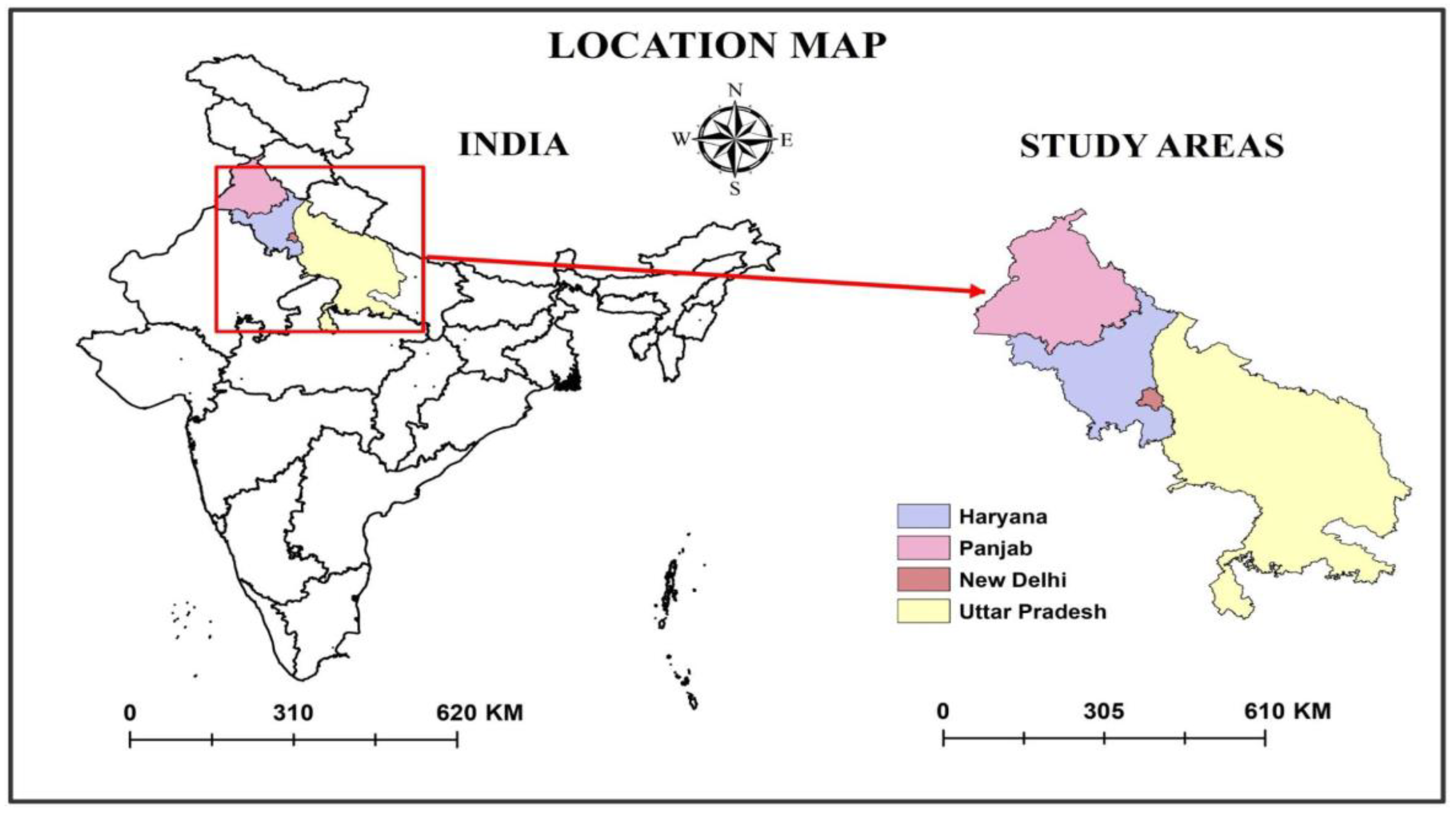
What forced the farmers across parts of Punjab, Haryana, and Uttar Pradesh to burn the stubble after harvesting yield in each season? This is a crucial issue that needs to be addressed before evaluating the air pollutants using geospatial technologies.
The reason behind the stubble burning in Punjab, Haryana, and Uttar Pradesh is that the farmers there have moved to specialized short-duration during Rabi (wheat) and Kharif (rice) growing seasons for increased crop yields. The cropping system allows time for the growing of two or more crops in a year. This generally takes June/July to October/November (Kharif season) for the rice crop, followed by November/December to March/April (Rabi season) for the wheat crop. It opens a short window of time for sowing wheat after the rice cropping season [
2]. However, a delayed sowing of wheat crops will adversely affect production and reduce crop yields. According to the Punjab Preservation of Subsoil Act of 2009, the paddy transplantation date is 20 June, pushing the rice harvesting date forward. Due to this law, farmers only have less than 20–25 days between two crops, so, given the unavailability of any cost-effective methods, burning is the only option left to them. This practice also cuts the labour cost from farmers’ perspectives and checks the growth of weeds, disease, and pests [
8]. Furthermore, this “cost-effective” agricultural approach results in a high cost to the environment and human health. Apart from causing air pollution, the burning of stubble also deprives the soil quality by burning the vital nutrients inside the soil and killing or displacing the essential microbes present in soil up to the depth of 2.5 cm because of increased temperature up to 42 °C [
9,
10]. This practice increases the additional expenses to the former in applying fertilizers or compost to restore the fertility of the fields. According to the published report by NPMCR [
11], the burning of 1oneton of stubble soil loses 5.6 kg of nitrogen, 2.4 kg of phosphorus, 25.5 kg of potassium, and 1.20 kg of sulfur [
12].
Severe haze is seen over the southern parts of the Indian Continent during the winter season [
13] because stubble fires have become rampant in Northern India (air mass movement carrying pollutants), especially in Punjab, Haryana, and some parts of western Uttar Pradesh. The low temperature in winter, especially from October to December, results in inversion conditions which act as a favourable condition for pollutants concentrating in the lower troposphere [
14], which leads to experiencing poor air quality in New Delhi and NCR (National Capital Region) that are listed among the top ranking most-polluted city areas in the world since 1990. In 2019, a global air quality report revealed that 14 of the world’s top 20 most polluted cities are in India, with Ghaziabad in Uttar Pradesh (UP) being the most contaminated [
15]. To maintain the air quality, central coordination is required to handle the problem, implying that the government would need to share the costs of compensation, abatement (lower stubble burning), or both in various ways. In general, incentive-based regulation could be cost-effective in reducing air pollution. As per Section 188 of the Indian Penal Code and the Air and Pollution Control Act 1981, 10 December 2015, the National Green Tribunal (NGT), it is illegal to burn stubble in open fields in Rajasthan, Uttar Pradesh, Haryana, and Punjab [
16]. Moreover, in 2014 the Union government released “the National Policy for Management of Crop Residue” to deal with stubble burning.
Physical ground-based monitoring for large areas is not possible using either fixed stations or movable instruments for a long period of time. These ground-based monitoring stations and instruments have certain limitations, such as higher maintenance costs and data point collections limited to small areas or only up to a few meters around the station resulting in discontinuous data incorporated to generate interpolated outcomes [
17]. The ground stations are limited in number and distributed unevenly, which provides data points, impeding the mapping of atmospheric pollutants as air quality varies frequently varies with regions [
18]. Atmospheric pollutants spread in a faraway place from emission source points of the pollutants through wind speed and direction as causing factors [
19]. Therefore, air mass movement and trajectory assessment are necessary to ascertain atmospheric pollutant concentration in a region for their movement and dispersal. Apart from main atmospheric pollutants, there are emissions of several kinds of hazardous pollutants nearby factories and industrial regions, such as Fluoride, which are harmful to humans, plants, and the surrounding environment [
20].
Earlier, Landsat 8 OLI data were employed to estimate the stubble burning area and its impact on the air quality index [
21]. Utilizing Earth Observation (EO) datasets for atmospheric pollutants monitoring provides continuous spatio-temporal data at different scales, i.e., the local to global scale [
22]. In recent decades, there has been increased and widespread use of EO datasets for the monitoring of atmospheric pollutants along with different algorithms and modelling techniques. Few researchers utilised the thermal infrared band from Landsat ETM sensors to monitor the distribution of PM
10 [
17]. Recently, researchers have utilised multi-sensor EO datasets such as IRS-P4 OCM, MODIS AOD, MOPITT CO, and OMI to monitor aerosol and CO transportation characteristics in the Indo-Gangetic plains over the Arabian sea [
23,
24]. Authors reported increased atmospheric pollutants in November [
23]. Some studies demonstrated the utilization of ground-based instruments for monitoring aerosols (High Volume Sampler-HVS) and NO
2 and SO
2 gases (using Thermoelectric Gaseous Attachments techniques) [
25]. Authors reported that the change in air chemistry just after the burning of crop residue was due to an increase in the concentration of SO
2 and NO
2 abruptly into the air. With the above discussion, it can be inferred that different EO and ground-based sensors and instruments are used for different parameters. However, with the launch of the Sentinel-5P instrument, major atmospheric pollutants can be monitored independently at a larger spatial extent in different periods. Though several articles were published for monitoring and observation of pollutants/air quality across the world and over India, no studies have yet exploited the advantages of the Sentinel-5P Tropomi/MODIS-derived MOD16A1 for the spatio-temporal monitoring of atmospheric pollutants due to stubble burning over the chosen site during 2018–2021.
The main objective of the present study was to monitor and investigate the spatio-temporal patterns of Sentinel-5P Tropomi based atmospheric pollutants, such as NO
X, SO
x, CH
4, CO, aerosols, and ozone (O
3) and the MOD64A1-derived burned area through cloud computing supported by the Google Earth Engine. This was performed in order to monitor the level of pollutants before and after stubble burning. Due to the movement and directions of the wind, pollutants are aggravated and circulate around the surrounding local states at a high level during the winter season. Trajectory frequency (HYSPLIT model) is utilised to assess the pollutant level through air mass movement. It was the first time implementing Sentinel-5P Tropomi to estimate the concentration of air pollutants due to stubble burning in parts of India. Several studies reported the air pollutants in terms of their concentration at ground level and monitoring of atmospheric concentration by use of preceding space-borne satellite data such as OMI, DOME, DOME 2, as discussed earlier [
26,
27,
28]. This attempt to identify changes in air pollutant concentrations at a spatial extent over time has been the subject of great interest and an important research theme. As mentioned above, the present work fills the gap between knowledge and estimation of air pollutants concentration due to stubble burning in India’s states.
3. Data Used and Methodology Adopted
The present study was conducted using the Google Earth Engine (GGE) and it used S5P and MODIS datasets for computational purposes. GGE is a cloud computing-based platform used to monitor and measure the change in the Earth’s environment at a planetary scale on a massive database of EO data. Thousands of computers in Google’s data centres are accessible via the platform, which intrinsically provides parallel-computing access. The platform also contains a new application programming framework, or “API”, available in Python and JavaScript that gives scientists access to these computing and data resources, allowing them to scale up or create new methods [
29]. Sentinel-5P was used for evaluating tropospheric data and MODIS MOD64A1 for burned data of the study site. The LULC map was generated for the study site for the year 2020, and later on, the agricultural area was extracted to illustrate how much area is used for agricultural practices. To estimate the burned area for the study site, we employed cloud-based computing for MOD64A1 monthly data for 2018, 2019, 2020, and 2021. It was performed to check the actual burned area in the study site and based on the results of the burned area. We extracted the month-wise data to evaluate the concentration and dispersion of the atmospheric pollutant for the years 2018, 2019, 2020, and 2021.
The Sentinel-5P TROPOMI: Tropospheric Monitoring Instrument was launched on 13 October 2017, at 2:57 p.m. IST as part of the Copernicus project. Sentinel-5P TROPOMI effectively observes concentrations of atmospheric pollutants and trace gases such as NO
2 Column Density, O
3 Total Atmospheric Column, SO
2, HCHO, CH
4, CO, Aerosol Absorbing Index (AAI), which are emitted into the atmosphere due to anthropogenic activities. Further, the instrument strengthens the assessment of aerosols and clouds. The specifications of Sentinel-5P TROPOMI are listed in
Table 1, along with the availability date of the data for particular pollutants.
Sentinel-5P TROPOMI-based datasets on the pollutant concentration levels were extracted and retrieved via cloud computing from the Google Earth Engine (GGE) (
https://code.earthengine.google.com/, accessed on 11 March 2021). GGE is a cloud-based platform widely used for processing satellite data. Sentinel-5P uses the TROPOMI instrument, a multispectral sensor that records the reflectance of wavelengths, optimised for measuring the atmospheric concentration of gases at a spatial resolution of 0.01 arc degree. The retrieval of the Sentinel-5P data was used for pre-processing, and the map generation was carried out using the SNAP and ArcGIS software, respectively.
To illustrate the spatio-temporal variation of major atmospheric pollutants due to the excessive stubble burning, the analyses of the above-mentioned analysis were obtained for different periods as listed above, corresponding to the stubble burning months, as shown in
Table 2 (for years 2018, 2019, 2020, and 2021).
Phase-1—the year 2018-(August to December 2018 based on data availability-
Table 1).
Phase-2—the year 2019 (January to December 2019).
Phase-3—the year 2020 (January to December 2020).
Phase-4—the year 2021 (January to December 2021).
The results/outcomes of major atmospheric pollutants are based on their data availability from Sentinel-5P Tropomi sensors.
4. Results
In this section, we will deal with the output generated for the LULC of the study site, the monthly burned area estimation for the years 2018, 2019, 2020, and 2021, and later, one of the Sentinel-5P Tropomi datasets which processed an estimation of the atmospheric pollutants generated from the study site, thus highlighting the impact of stubble burning using Earth observation datasets, i.e., MOD64A1 and S5P-Tropomi.
4.1. LULC for the Study Site
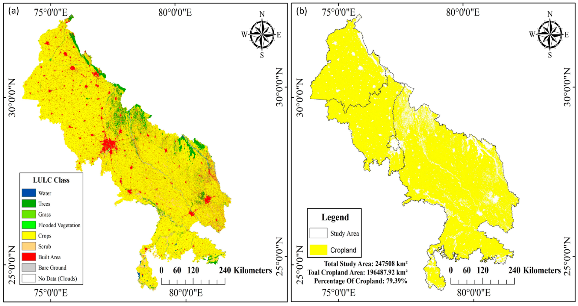
LULC is generated for the identification of land cover in the study sites from the ESRI LULC2020 product [
30] that establishes the baseline information for mapping and change analysis [
31,
32]. LULC for the study site was created to assess the utilization of land for different purposes, such as agriculture, urban areas, water bodies, forests, and so on, for activities such as thematic mapping and change detection analysis. The main purpose of LULC in the present study is to delineate or estimate the total agricultural area where there is a chance of possible stubble burning. The LULC map was derived from the ESA Sentinel-2 imagery at a 10 m spatial resolution from ESRI2020 [
30], representing crops, water bodies, vegetation, flooded vegetation, scrub, built-up areas, and bare ground (the land cover types were considered from the ESRI land cover products). As we aimed to assess the impact of stubble burning, we mainly focused on the agricultural area through the LULC of the study sites for 2020 (as shown in
Figure 2a). The agricultural area was extracted from the derived LULC to determine the total area of agricultural practices in the study site and individual states. The agricultural area accounts for 38,154.66 km
2 for Haryana, 42,888.15 km
2 for Punjab, 436.23 km
2 for New Delhi, and 176,531.80 km
2 for Uttar Pradesh in the year 2020, as calculated and extracted from the LULC outputs (refer to
Figure 2b). The stubble burning is mainly carried out in Punjab and Haryana, with only small instances of burning in only a few parts of Uttar Pradesh.
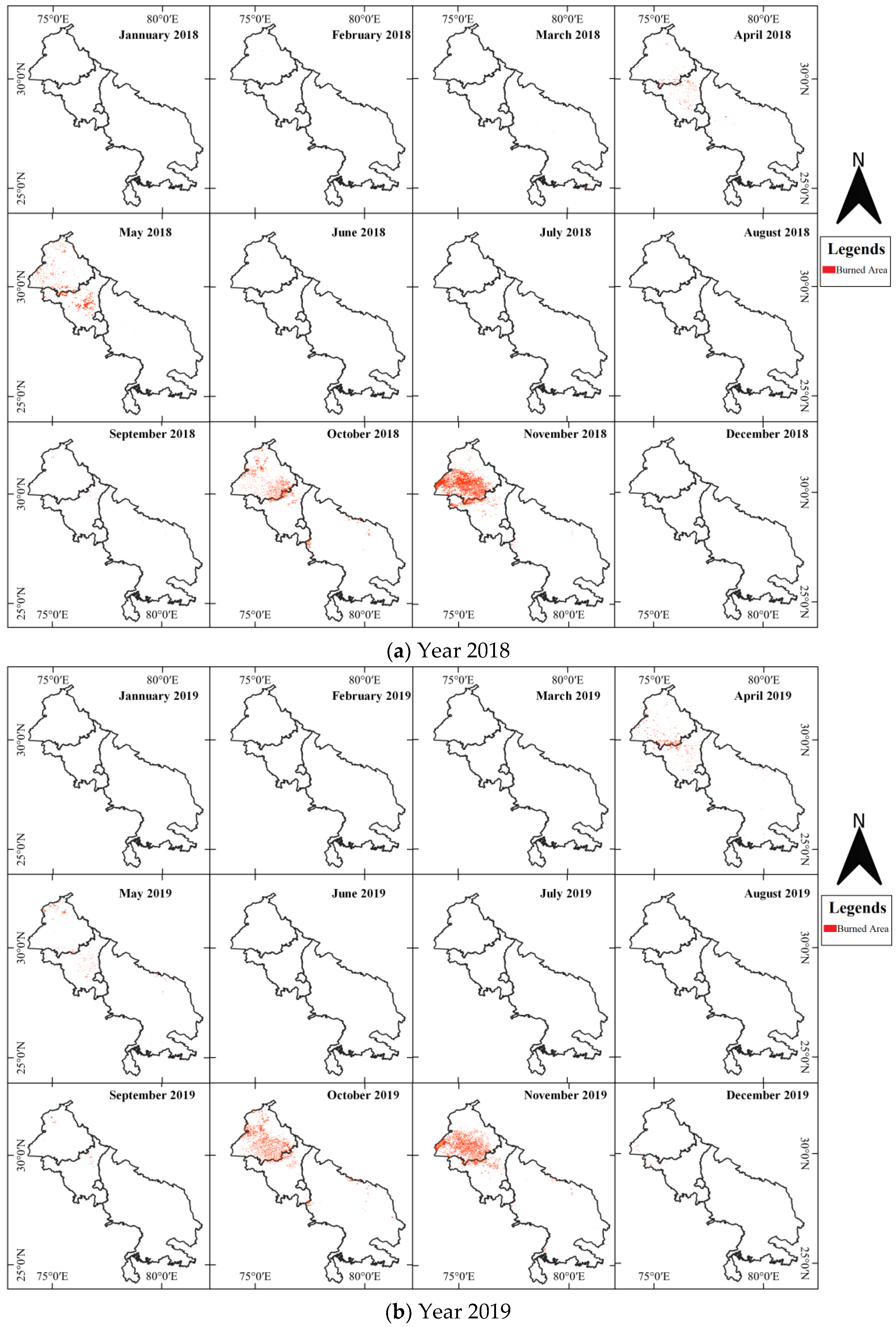
4.2. Burned Area for the Study Sites (the Years 2018, 2019, 2020, and 2021)
This section identifies the stubble burning months for each year by using Moderate Resolution Imaging Spectro-radiometer (MODIS) MCD64A1 data. Kharif crops are sown during early May and late June, for which fields need to be cleared of stubble, and the subsequent stubble burning (the burning of refuses after Rabi crop harvesting) can be seen during the AMJ months. Similarly, Rabi crops are sown in late October and late November, which results in quick stubble burning (the refuses from Kharif harvested crops preferably after monsoon rains) across the major parts of the country. The time gap between Rabi crop planting and Kharif crop harvesting is approximately two to three weeks, and the field needs to be prepared. This is considered to be a fast clearing method by the farmers to prepare the field for the new crops [
33]. We had reviewed several published pieces of literature to precisely focus on the month when agricultural residues were burnt in the study sites [
33,
34,
35]. Based on month-wise burned area estimation, we have defined the span period for assessing pollutants using Sentinel-5P (as shown in
Table 1 and
Figure 3).
MODIS-Surface Reflectance imagery provides the MCD64A1 burned-area gridded data, which helps estimate active fires [
36]. We have used cloud-based computing to generate estimates of the active burn regions in the study site, using algorithms that include the burn date for the 500 m-grid cells within the MODIS tile. As MODIS is the exclusive fire monitoring sensor and has the capability to estimate or detect fires in a small area precisely when compared to the other existing Earth observation sensors.
The information is available in the MOD64A1 product version 6 data layers, including Burn Date, Burn Data Uncertainty, Quality Assurance, and Julian day (1 to 365) of the concerned year (data availability from January 2000 to present).
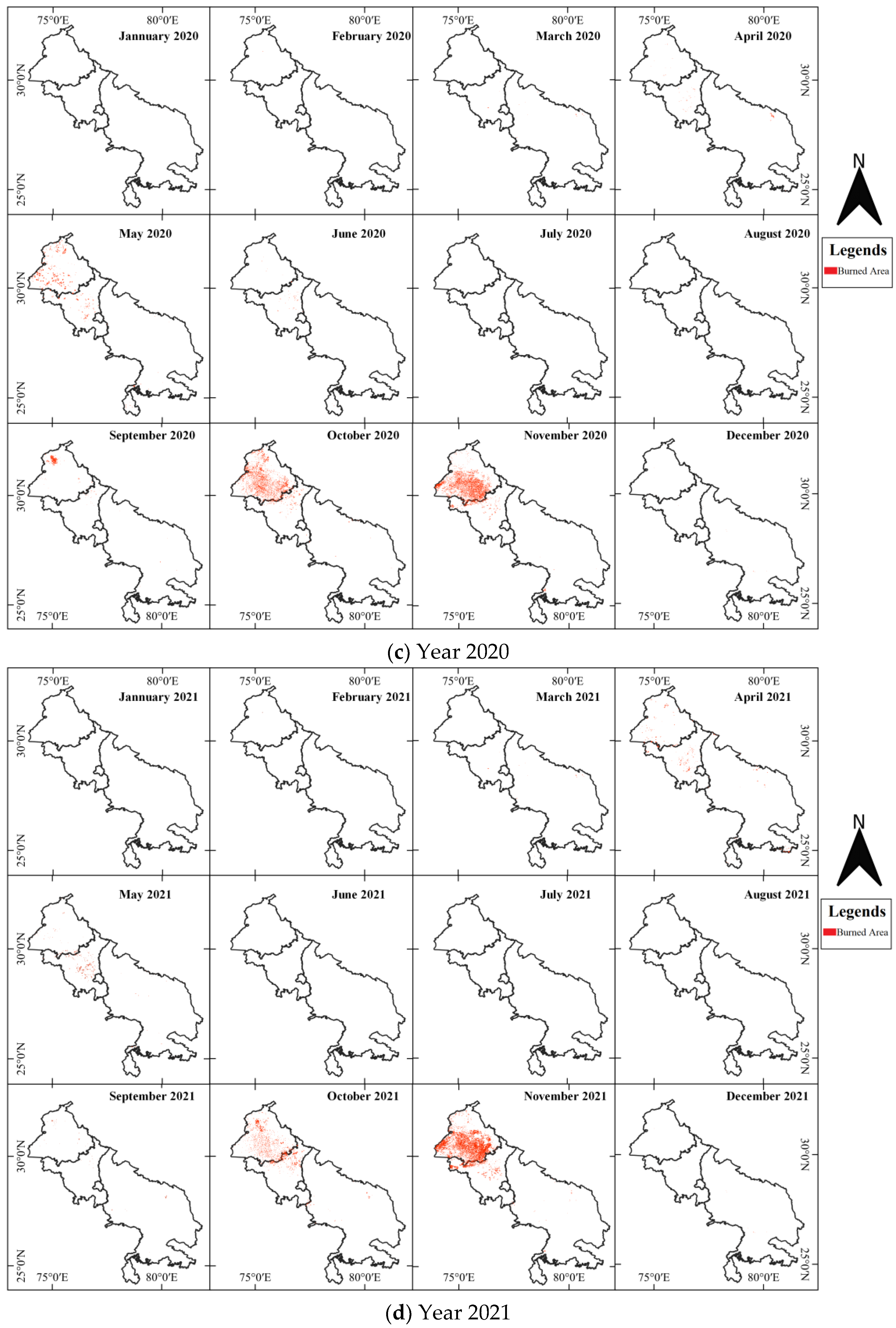
MODIS data illustrate that the stubble burning cases were recorded in April, May, and June (OMJ-Months) as well as during October, November, and December (OND-Months) for 2018, 2019, 2020, and 2021. These months of 2018, 2019, 2020, and 2021 were considered severe because stubble burning added more carbon to the atmosphere than in other months. We have tried to classify three-time periods based on our understanding of atmospheric pollutants linked with seasonal variation, with higher atmospheric concentrations during post-monsoon/winter and lower during pre-monsoon seasons [
23,
34].
As previously discussed, we have included the above period of April to June and September to December in highlighting the atmospheric pollutants using the Sentinel-5P datasets as described below:
Spring period: As seen from
Figure 2 (MODIS Burned area), the data demonstrates that burn areas were detected in April, May, and June due to the burning of post-harvest residue leftover from Kharif crops, such as as rice. During this period, stubble burning will not aggravate the problems.
The summer/monsoon period: Another reason for less burning in the rainy season, as it brought down stubble burning incidents. Stubble burning usually occurs until May 15 in North India as farmers prepare their fields for Kharif crops. However, this does not lead to acute pollution because of the high temperature and high dispersion rates.
Post-Monsoon and Winter period: Stubble burning takes place in September, October, and November across the study area as farmers involved in agricultural practices prepare their fields for Rabi crops, such as wheat. During this period, the impact of stubble burning is more severe because the lower temperature in winter leads to a stable environment (inversion condition) [
14]. The rice stubble burning is higher than wheat and, in the inversion condition, favours the pollutant to stay longer in the atmosphere, creating a massive visibility problem in the capital region and degrading the Air Quality Index (AQI) during this period [
21]. Thus, OND months present with a high concentration of pollutants. Stubble burning alone is not the only factor affecting post-monsoon air quality in the study area; other factors, including ambient temperature, relative humidity, wind speed, wind direction, and ambient pressure, also play an important part [
37].
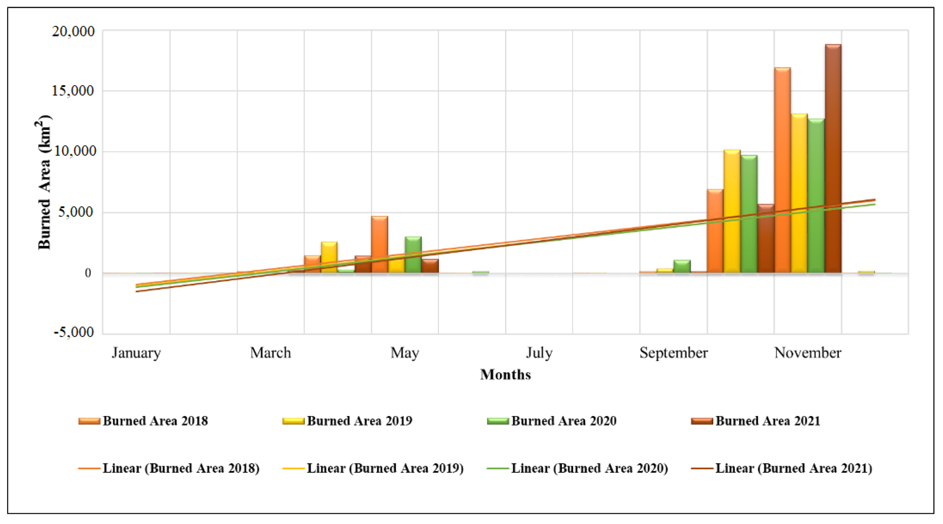
The data processed from MODIS shows that the total burned area for 2018, 2019, 2020, and 2021 are 30,422.5 km
2, 27,956 km
2, 27,084.5 km
2, and 27,591.5 km
2. In which the AMJ share for each year is 20.44%, 14.65%, 12.73%, and 9.49% (as offline/real-time data were not available for December 2021, it was reported until November 2021), respectively, and OND shares are 78.44%, 83.44%, 82.94%, and 88.84%, respectively (refer to
Figure 4). As seen in
Figure 4, April–May–June and October–November–December during 2018, 2019, 2020, and 2021 correspond to the highest burned area in the study site, as seen in
Table 2.
4.3. Sentinel-5P TROPOMI Derived Results for Major Pollutants
This section deals with the estimation of atmospheric pollutants using Sentinel-5P data through the use of cloud computing. Indicators of atmospheric pollution due to stubble burning can be assessed using the Sentinel-5P TROPOMI data.
4.3.1. Aerosol Estimation
The
Aerosol Index Product provided by S5P TROPOMI is a qualitative index that measures the presence of aerosols with substantial absorption. Mathematically, the aerosol Index can be expressed by:
AAI is the aerosol absorbing Index; R
meas depicts measured reflectance at wavelengths
λ1 and
λ2; R
calc describes calculated reflectance from the atmosphere with Rayleigh scattering; A
LER is the Lambert equivalent reflectivity, which is the measured reflectance for wavelength
λ2. The aerosol concentration range varies from −21 (min) to 39 (max). The aerosols that absorb light (dust and smoke) are represented by positive values of the Aerosol Index, while tiny or negative values represent non-absorbing aerosols and clouds. If the Index of refraction, particle size distribution, and the height of the aerosol layer are known from previous measurements, the Index can be interpreted in terms of optical depth [
38].
The S5P TROPOMI instrument estimates the Aerosol Index (AI) using two wavelength ranges. Therefore, AI is calculated using the 340 nm and 380 nm wavelengths from the S5P Tropomi instrument. AI
340/380 and AI
354/388 are provided to the users in the Level-3 product in the cloud computing platform for analysis at spatial scale (as L2 products are binned at the time and not at spatial scale). Offline AI data from July 2018 to December 2021 were collected for analysis.
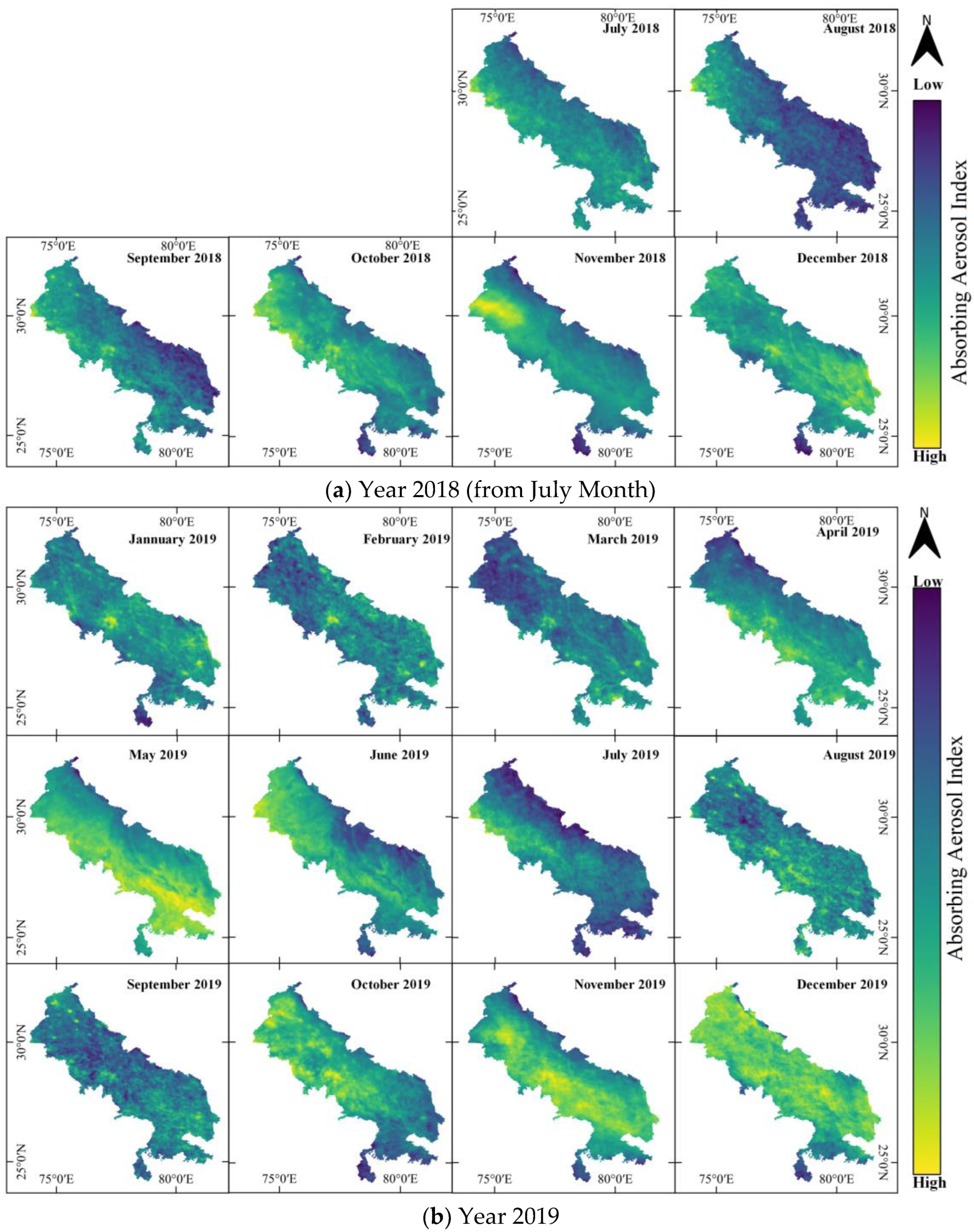
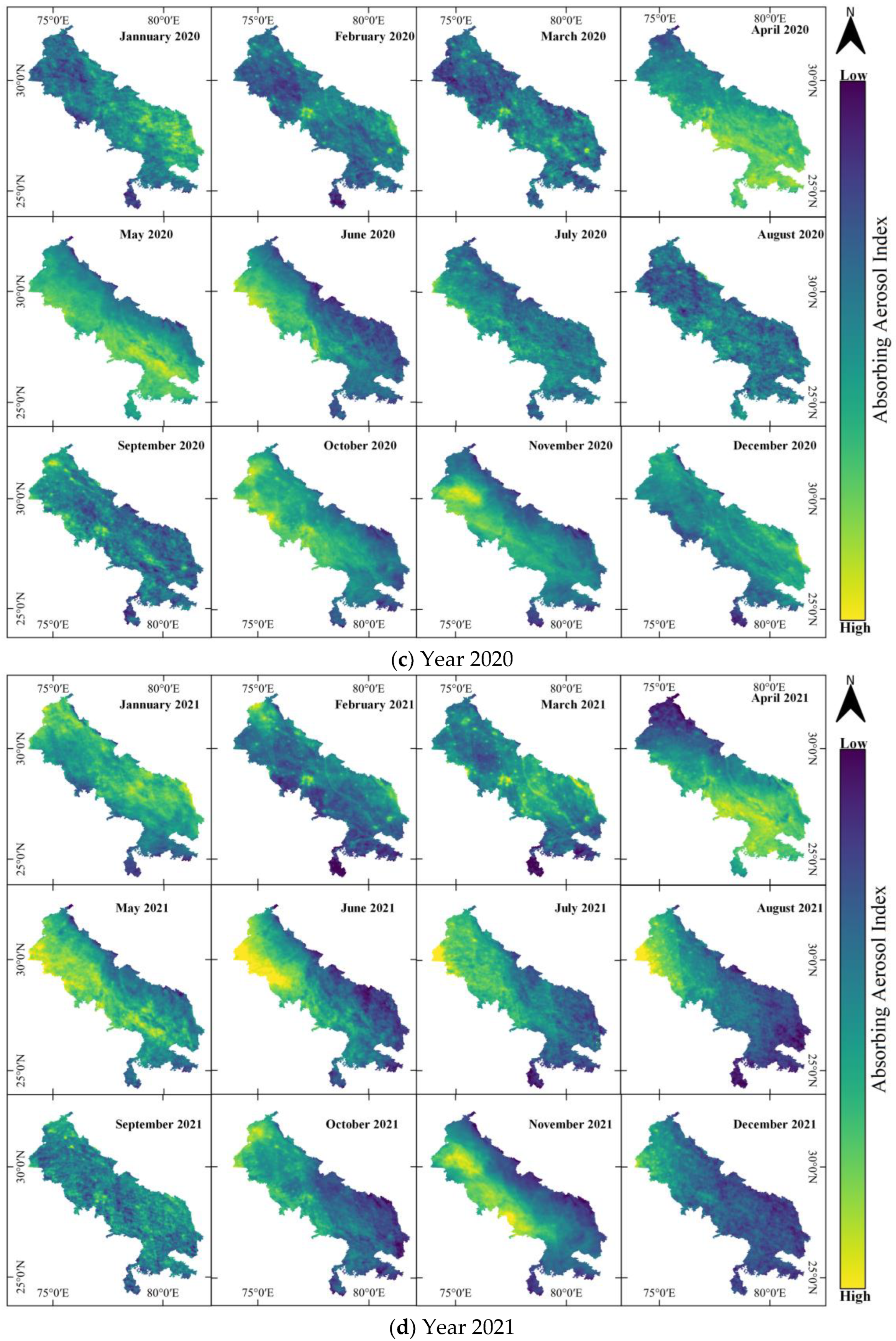
Figure 5. illustrates the concentration of the Aerosol Index from 2018 to November 2021. The results showed that the maximum concentrations were seen in April, May, and June (AMJ) and during winter, October through to December (the OND months of each year). Sentinel5P can achieve a maximum value of 39 for the Aerosol index. Our findings show that the AI for the AMJ months was found to be 0.11, 0.24, and 0.15 for the years 2019, 2020, and 2021, while those for OND months are 0.99, 1.58, 1.63, and 1.90 for the years 2018, 2019, 2020, and 2021, respectively. Our findings reported that the concentration was found to be higher in the OND months (winter) followed by the AMJ months of each year, as seen in
Figure 5.
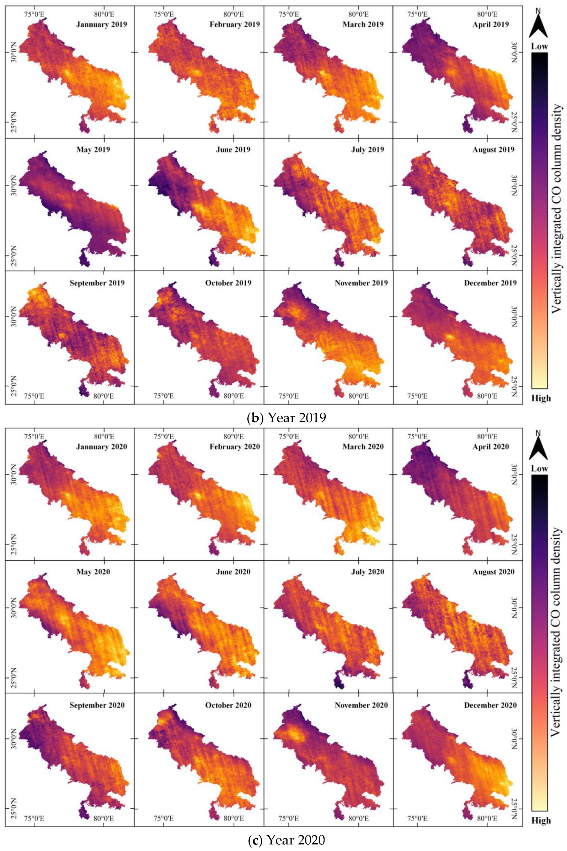
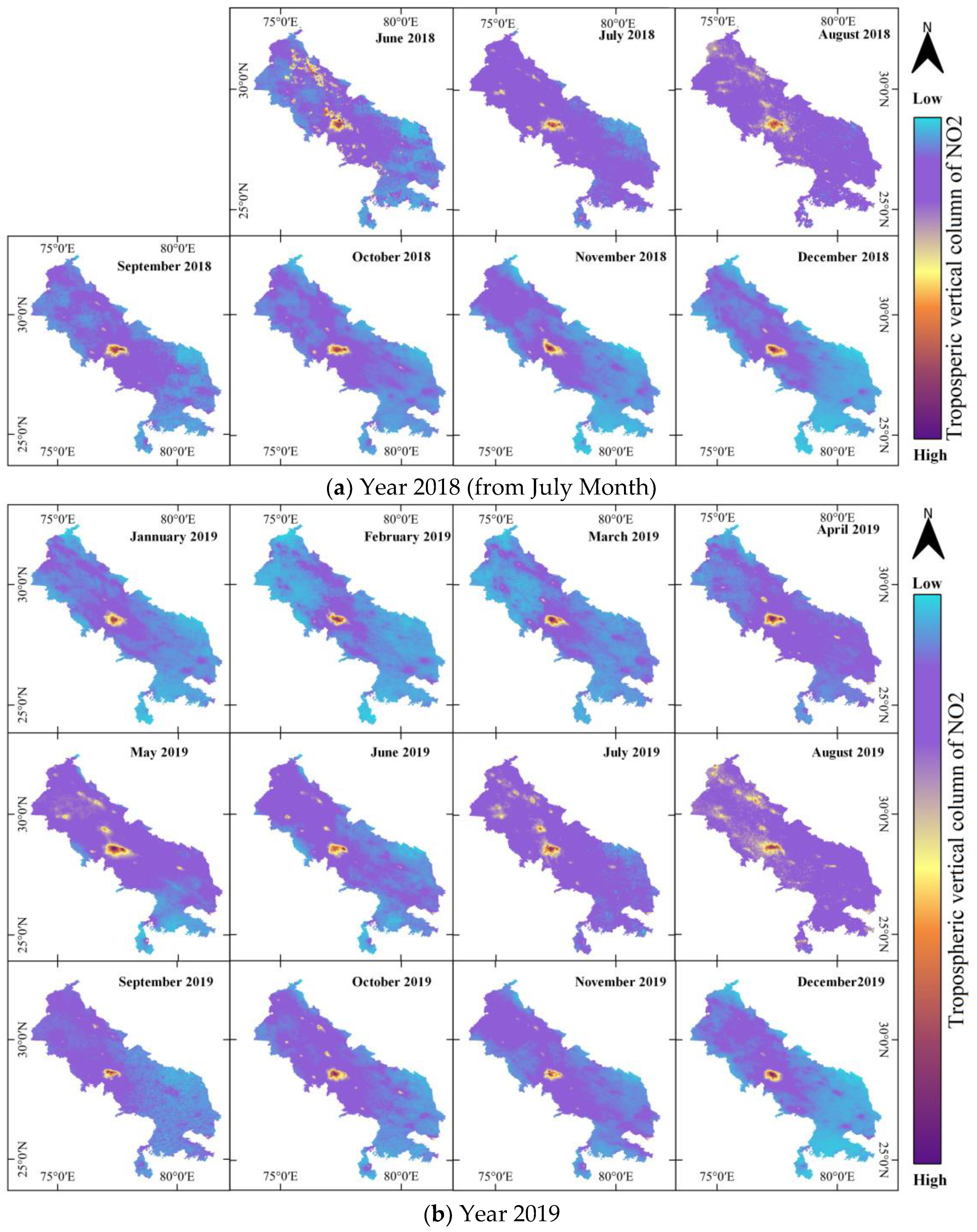
4.3.2. CO (Carbon Monoxide)
The
Carbon Monoxide Product is used to estimate the total column that needs to be retrieved for background CO abundance and surface reflection. A physics-based retrieval approach was used to derive the scattering properties of the observed atmosphere and associated trace gases in the atmosphere [
39]. Carbon monoxide (CO) is an important atmospheric trace gas for understanding tropospheric chemistry. In some urban regions, it is a major atmospheric pollutant. The primary sources of CO are the combustion of fossil fuels, biomass burning, and the atmospheric oxidation of methane and other hydrocarbons. Whereas fossil fuel combustion is the primary source of CO in northern mid-latitudes, the oxidation of isoprene and biomass burning play an essential role in the tropics. TROPOMI on the Sentinel 5 Precursor (S5P) satellite observes the CO global abundance exploiting clear-sky and cloudy-sky Earth radiance measurements in the 2.3 µm spectral range of the shortwave infrared (SWIR) part of the solar spectrum [
40]. S5P TROPOMI clear sky observations provide CO total columns sensitive to the tropospheric boundary layer [
41].
The column sensitivity changes according to the light path for cloudy atmospheres and is thus easy to estimate using SP5 datasets. Here, Sentinel-5P is employed to estimate the vertically integrated CO column density at 0.01 arc degrees, which provides the CO concentrations ranging from a minimum of 0.01 to a maximum reported value of 5.71 mol/m
2. Offline CO data from June 2018 to December 2021 were collected for analysis.
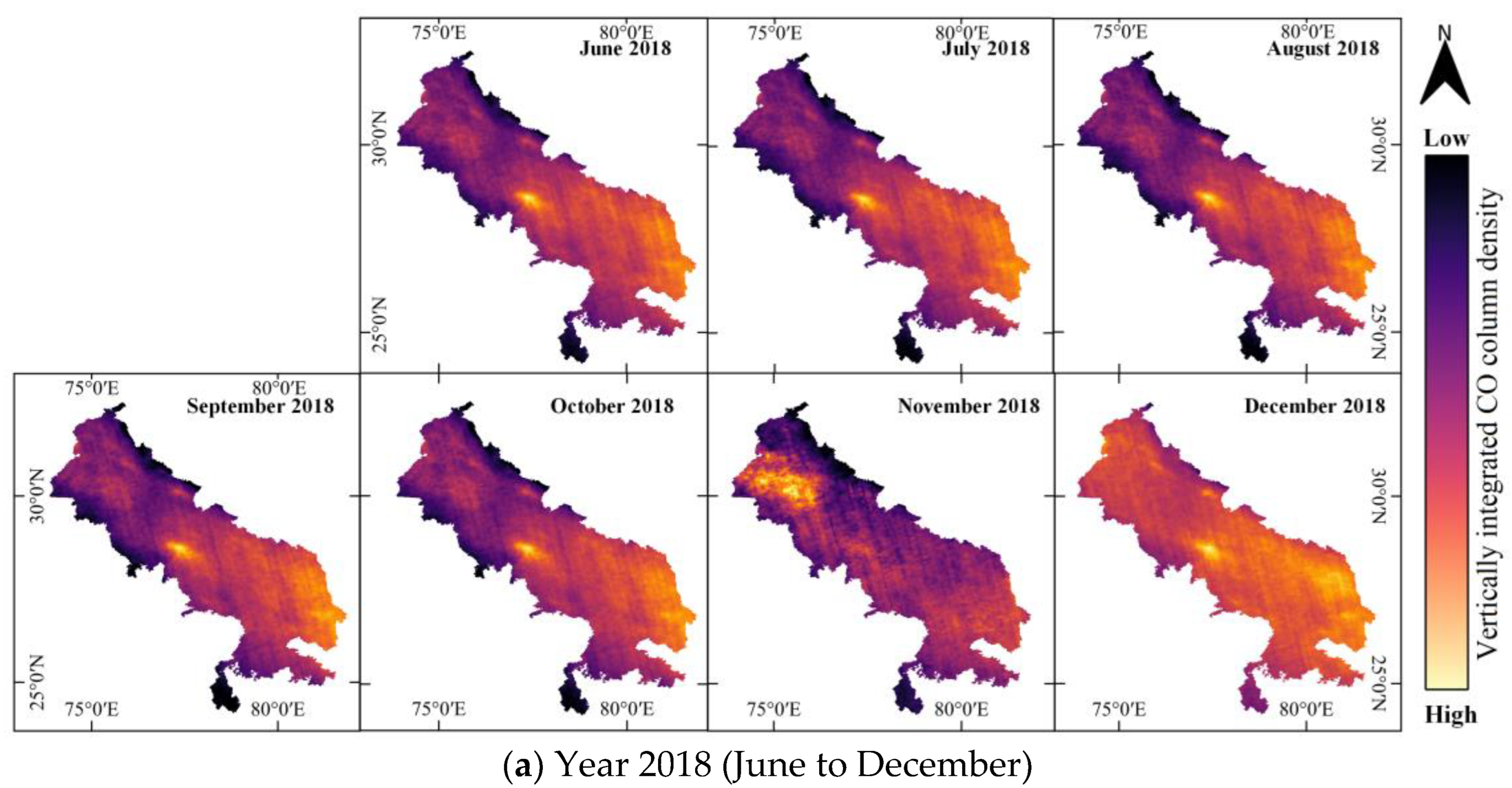
Figure 6 illustrates the CO concentration from November 2018 to November 2021. The results showed that the maximum concentrations were seen in April, May, and June (AMJ) and during winter, October through to December (OND months) each year. The average value of CO concentration in the study area was found to be 4.6 × 10
−2 mol/m
2. The CO concentrations for the AMJ months are found to be 4.8 × 10
−2, 4.54 × 10
−2 and 4.59 × 10
−2 for the years 2019, 2020, and 2020 while, it was found to be 5.16 × 10
−2, 4.98 × 10
−2, 5.44 × 10
−2 and 5.46 × 10
−2 mol/m
2 for the OND months for the years 2018, 2019, 2020, and 2021, respectively. The results concluded that CO concentrations were found to be slightly higher in thr OND months (winters) as compared to AMJ months in each year, as seen in
Figure 6.
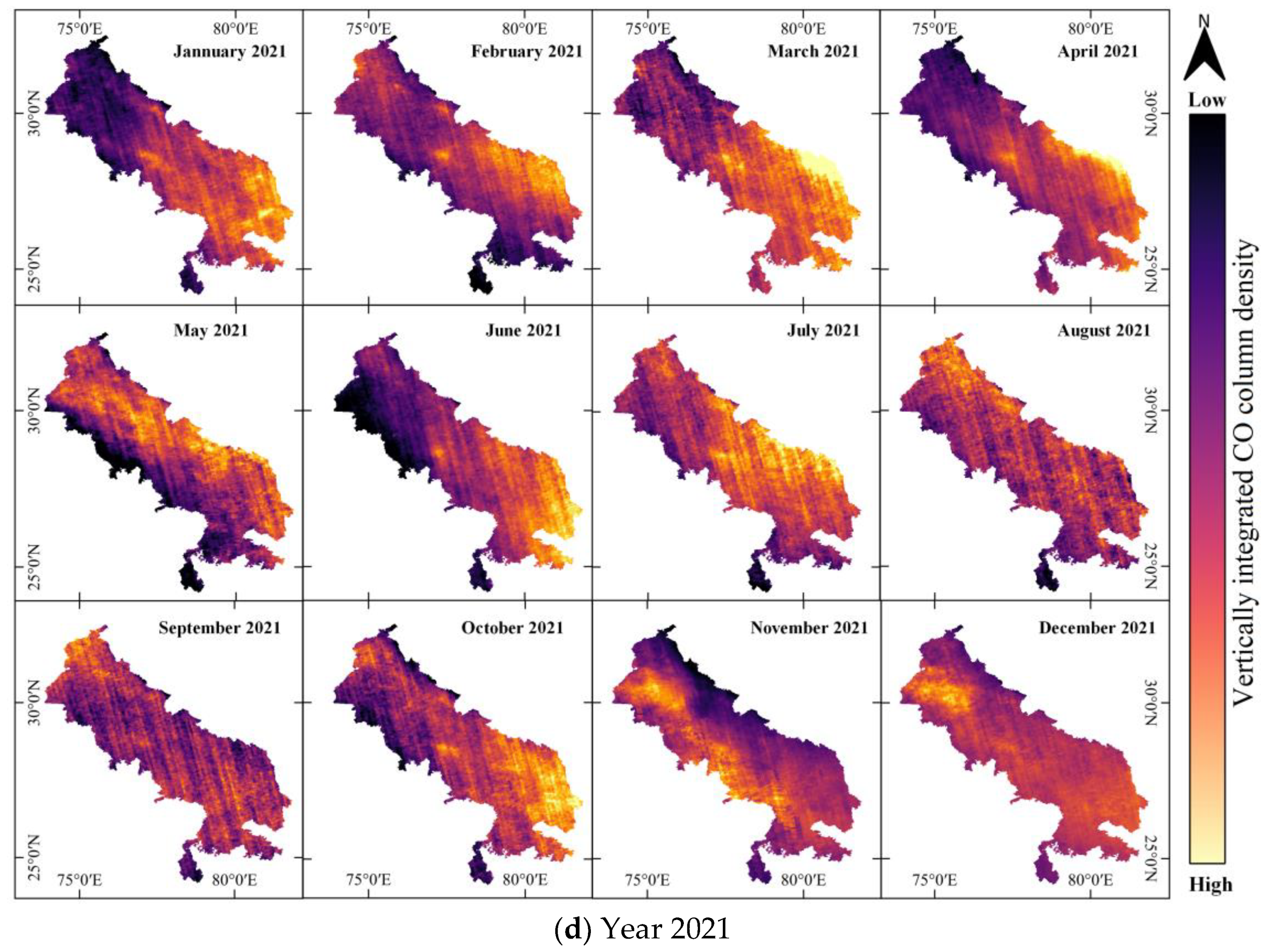
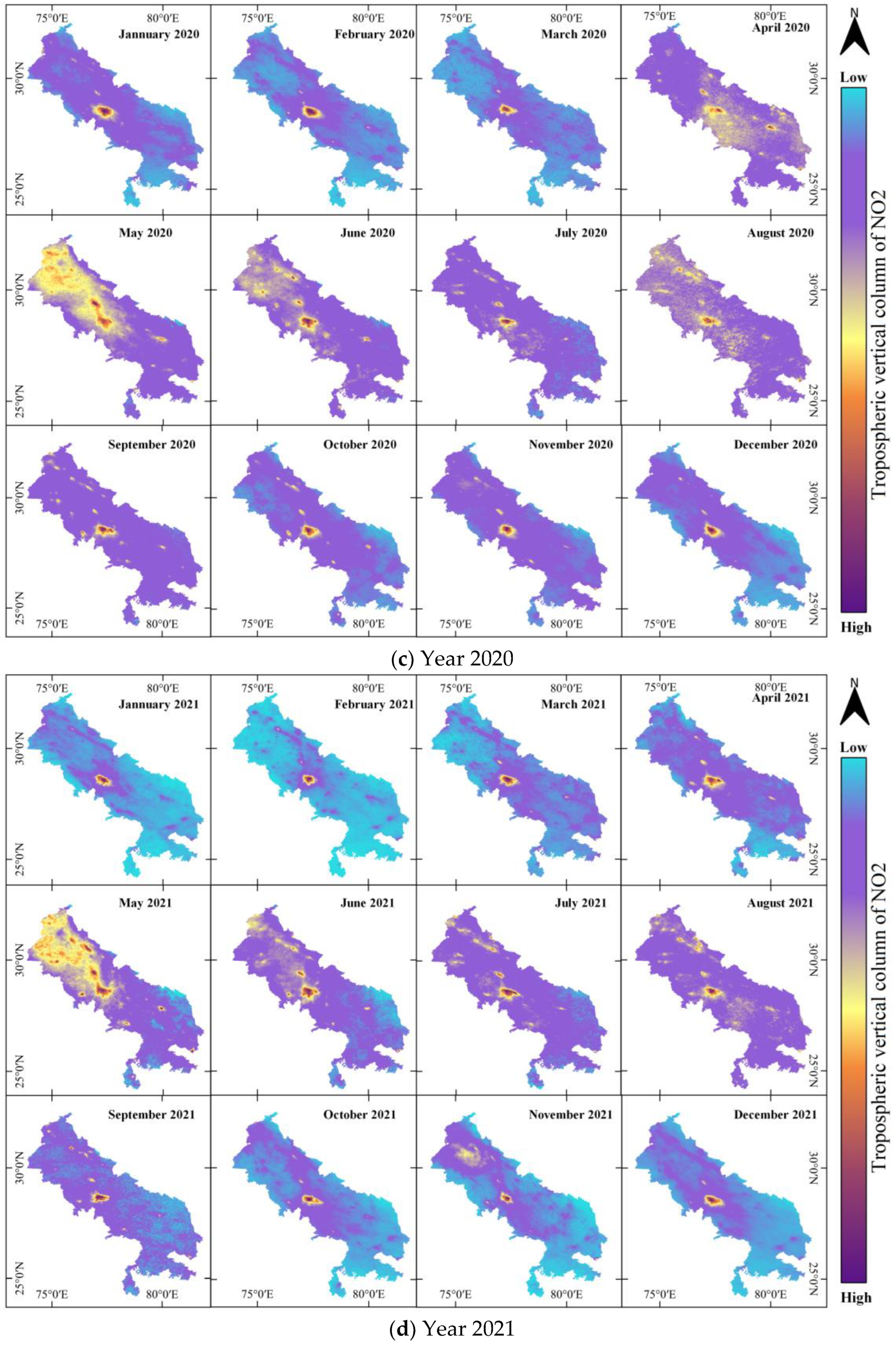
4.3.3. Oxide of Nitrogen (NO2/NO)
Oxides of nitrogen (such as nitrogen dioxide (NO
2) and nitrogen oxide (NO)) are significant trace gases that are the end products of anthropogenic sources as well as natural processes. These are emission gases that are harmful to the atmosphere, which cause smog, acid rains, and other related problems. Nitrogen oxides (NO
2 and NO) are important trace gases in the Earth’s atmosphere, present in the troposphere and the stratosphere. These gases enter the atmosphere due to anthropogenic activities (fossil fuel combustion and biomass burning) and natural processes (wildfires, lightning, and microbiological processes in soils) [
42]. Here, NO
2 is used to represent the concentrations of collective nitrogen oxides because during the daytime, i.e., in the presence of sunlight, a photochemical cycle involving ozone (O
3) converts NO into NO
2 and vice versa on a timescale of minutes. The TROPOMI NO
2 processing system is based on the algorithm developments for the DOMINO-2 product, and the EU QA4ECV NO
2 re-processed dataset for OMI and has been adapted for TROPOMI. This retrieval-assimilation-modelling system uses the three-dimensional global TM5-MP chemistry transport model at a resolution of 1 × 1 degree as an essential element. Here, Sentinel-5P is employed to estimate the total vertical column of NO
2 (ratio of the slant column density of NO
2 and the total air mass factor) at 0.01 arc degrees. The tropospheric NO
2 column number density ranges from minimum values of −5.37 × 10
−4 to maximum reported values of 1.92 × 10
−2 (mol/m
2). However, from December 2020 onwards, there have been changes and improvements in the S5P NO products [
43,
44,
45]. The offline NO
2 data from June 2018 to December 2021 were collected for analysis (refer to
Table 1 for more information).
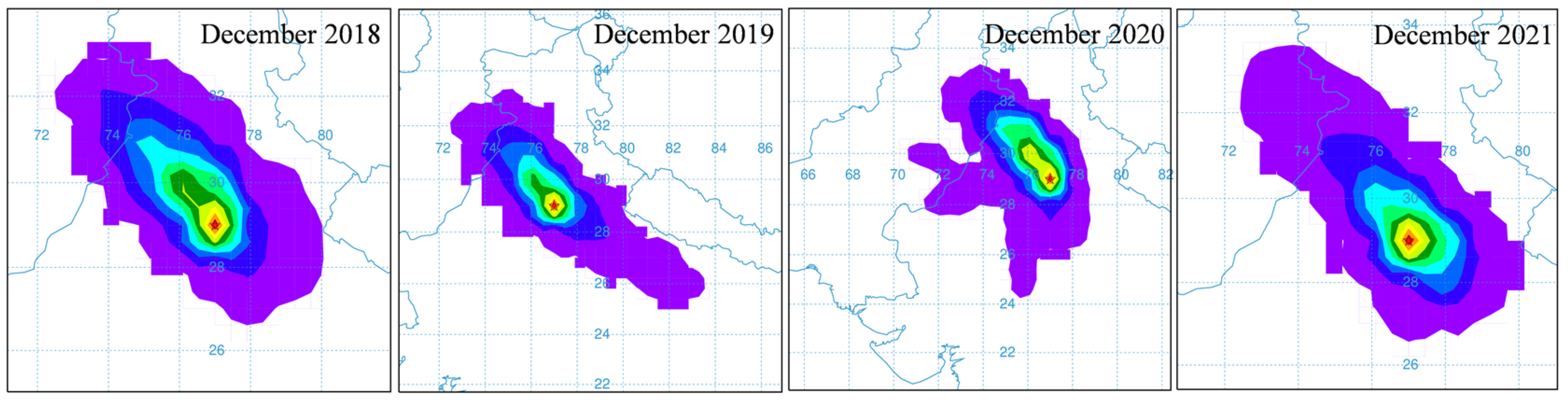
Figure 7 demonstrates NO
2 concentration from November 2018 to November 2021. The results showed that maximum concentration was seen in April, May, and June (AMJ) and during winter, October through to December (the OND months of each year). The concentration in winter is slightly higher than the AMJ months in each year, as seen in
Figure 7. The amount of NO
2 in the atmosphere is linked to several emission sources, such as vehicular emissions and natural sources. The average NO
2 concentration in the study area was found to be 2.02 × 10
−4 mol/m
2. The concentrations for the AMJ months are 1.27 × 10
−4, 1.75 × 10
−4, 9.32 × 10
−5 and 1.26 × 10
−4 mol/m
2 and for the OND months are 3.37 × 10
−4, 2.87 × 10
−4, 2.26 × 10
−4 and 2.62 × 10
−4 mol/m
2 for the years 2018, 2019, 2020, and 2021, respectively.
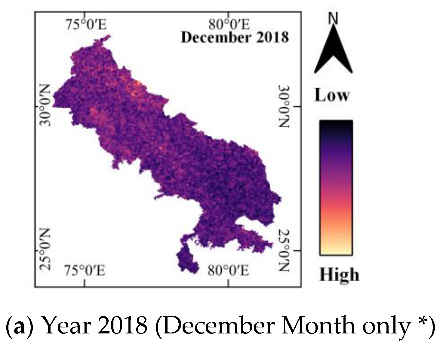
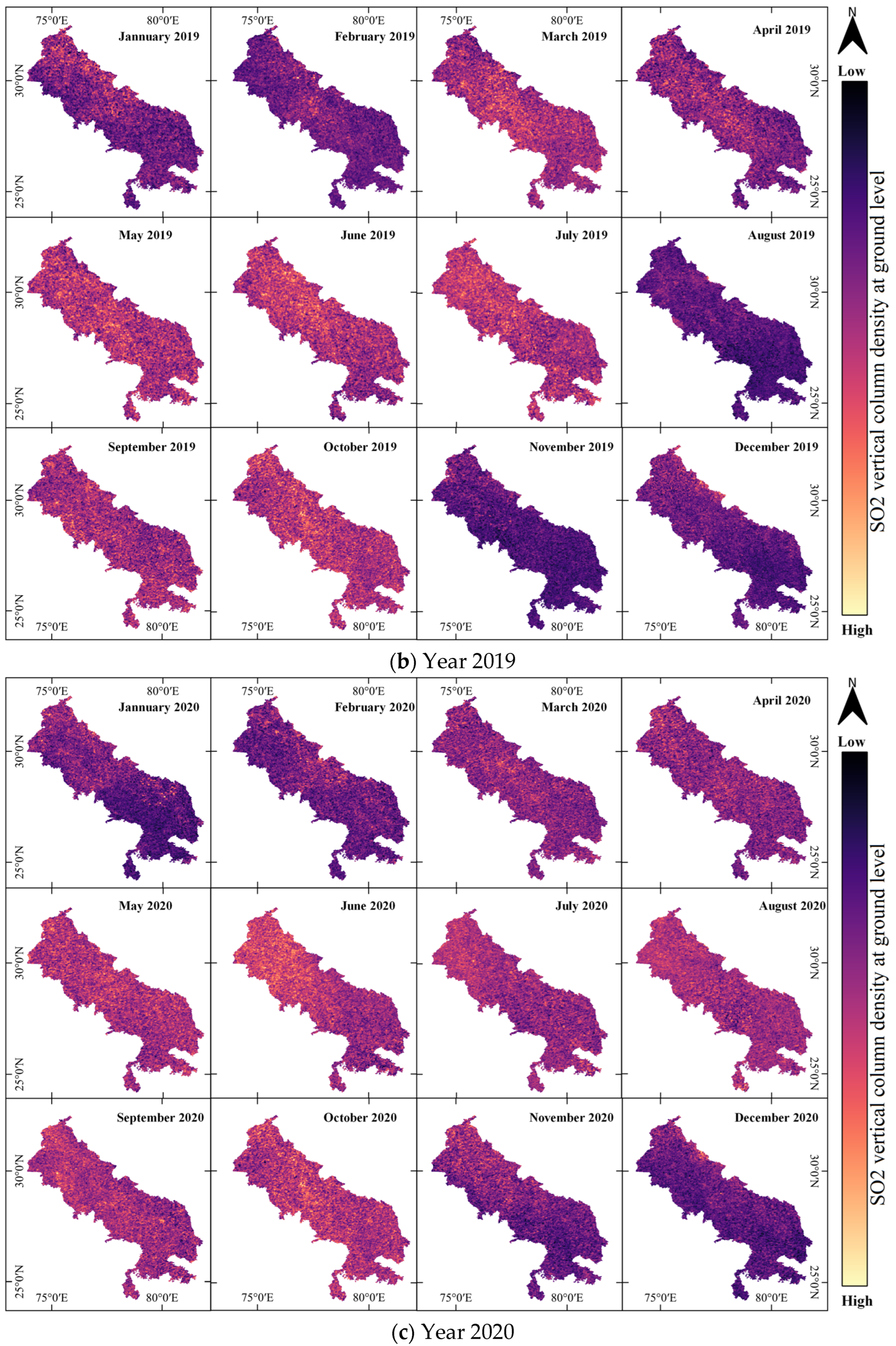
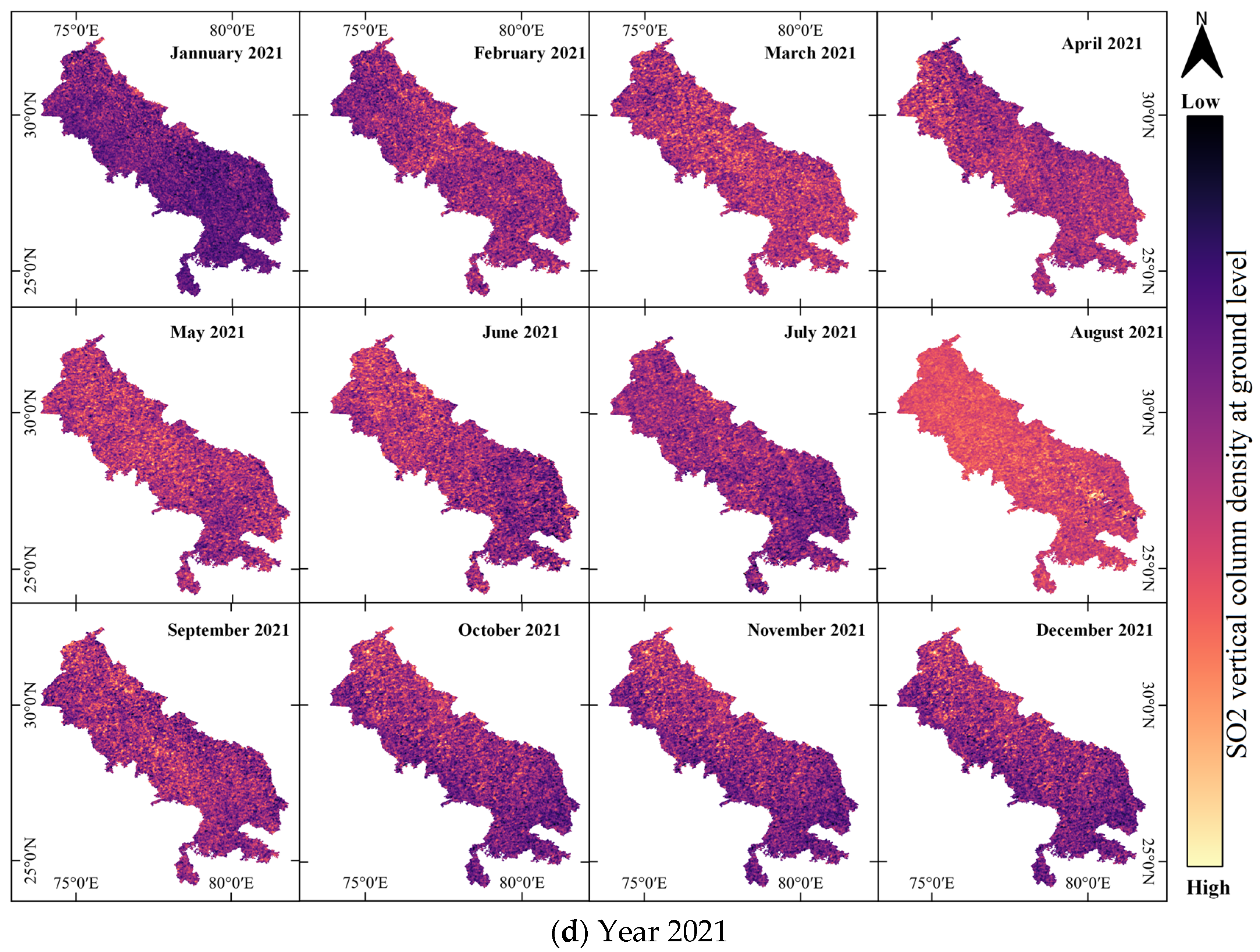
4.3.4. Oxide of Sulfur (SO2)
Sulfur dioxide (SO
2) enters the Earth’s atmosphere through natural and anthropogenic processes. It plays a role in chemistry on a local and global scale, and its impact ranges from short-term pollution to effects on the climate. The sources of the increased concentration of SO
2 in the atmosphere are attributed to anthropogenic sources, vehicular emissions, biomass burning, and fossil fuels combustion) [
46] and natural phenomena (lightning, forest fires, microbial activities, and other means). Only about 30% of the emitted SO
2 comes from natural sources; most are anthropogenic. SO
2 emissions adversely affect human health and air quality. SO
2 affects climate through radiative forcing via the formation of sulfate aerosols. Volcanic SO
2 emissions can also pose a threat to aviation, along with volcanic ash. S5P/TROPOMI samples the Earth’s surface with a revisit time of one day with an unprecedented spatial resolution of 3.5 × 7 km, which allows the resolution of fine details, including the detection of much smaller SO
2 plumes. More information about the datasets and their processing can be checked at GGE.
Here, S5P TROPOMI is employed to estimate the SO
2 vertical column density at ground level, calculated using the DOAS technique at 0.01 arc degrees, ranging from 0.4051 to 0.2079 (mol/m
2) as reported by S5P-Tropomi outcomes. The weighted mean of cloudy and clear air mass factor (and) weighted by intensity-weighted cloud fraction ranges from 0.1 to 3.387 (mol/m
2) and can be measured using Sentinel-5P. Offline SO
2 data from December 2018 to December 2021 were collected for analysis. The average SO
2 was found to be 9 × 10
−4 mol/m
2 over the study area and for AMJ months 5.4 × 10
−4, 5.61 × 10
−4 and 5.59 × 10
−4 mol/m
2 and for OND months 1.55 × 10
−3, 1.32 × 10
−3 and 8.9 × 10
−4 mol/m
2 of 2019, 2020, and 2021, respectively.
Figure 8 demonstrates SO
2 concentration from December 2018 to November 2021. The results showed that the maximum concentration was seen in the months of AMJ as well as during the winter, October through to December (OND) each year. The concentrations in winter were slightly higher than those of the AMJ months of each year, as seen in
Figure 8. The amount of SO
2 in the atmosphere is linked to several emission sources, such as vehicular emissions and even natural sources.
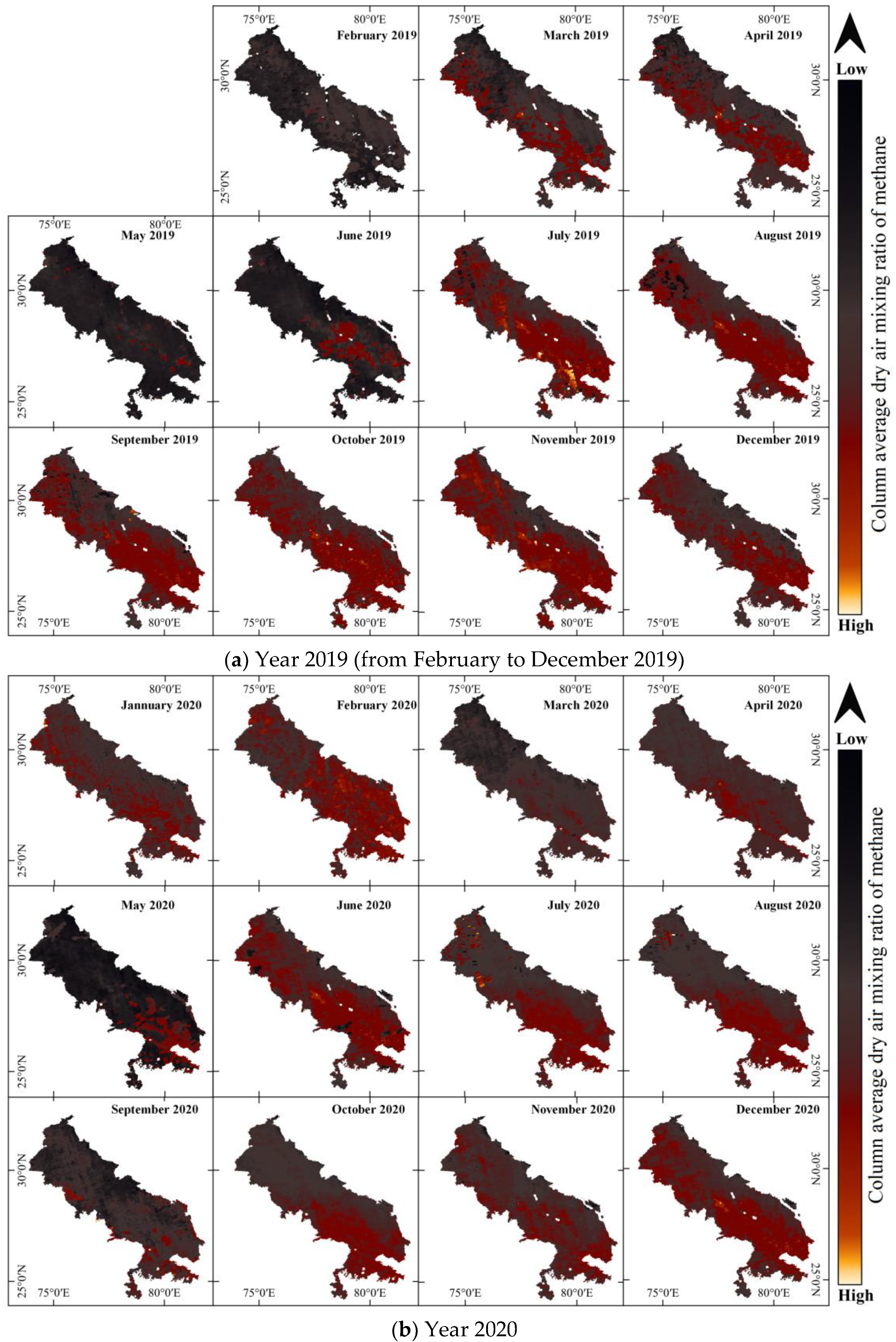
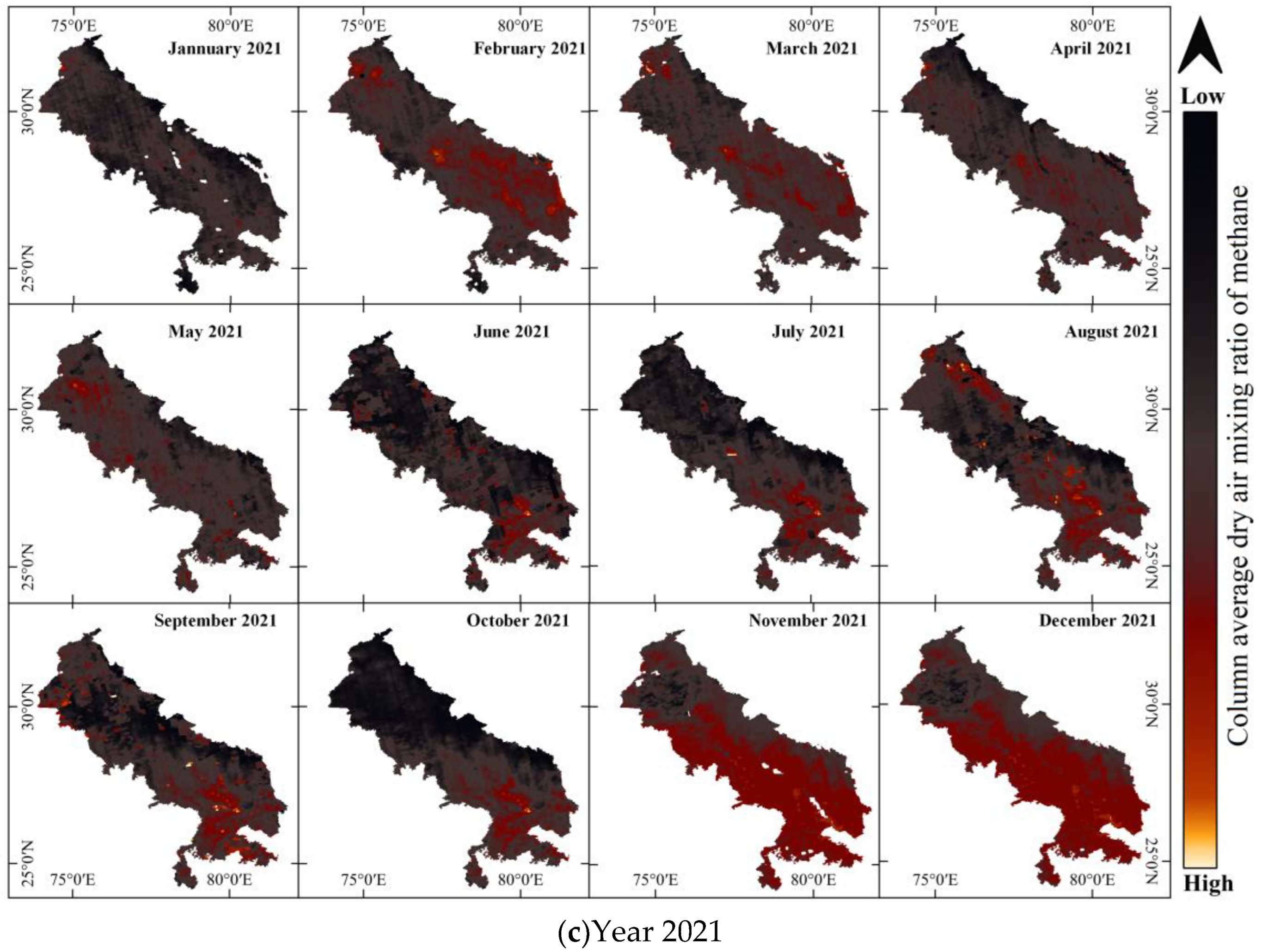
4.3.5. Methane (CH4)
Methane (CH
4), after carbon dioxide (CO
2), is the largest contributor to greenhouse gases (GHGs) from anthropogenic emissions, which causes a global warming effect [
30,
47]. Roughly three-quarters of CH
4 emissions are anthropogenic, so it is essential to continually record satellite-based measurements. TROPOMI aims to provide CH
4 column concentrations with a high sensitivity to readings from the Earth’s surface, good spatiotemporal coverage, and sufficient accuracy to facilitate the inverse modelling of sources and sinks. The offline CH
4 data from February 2019 to December 2021 were collected for analysis. TROPOMI uses absorption information from the Oxygen-A Band (760 nm) and the SWIR spectral range to monitor CH
4 abundances in the Earth’s atmosphere [
48]. Some filters need to be applied to remove the bad pixels, but filtering on a value of <0.5 does not remove all the pixels considered useless. Some pixels with too low of a methane concentration are still present: (a) Single TROPOMI overpasses show stripes of erroneous CH
4 values in the flight direction. Secondly, not all pixels above inland bodies of water are filtered out. Here, Sentinel-5P is employed to estimate methane’s column-averaged dry-air mixing ratio at 0.01 arc degrees, ranging from 1491 to 2352 (ppbV) (refer to
Figure 9). The average CH
4 was found to be 1967.12 ppbV for the study area and for the AMJ months 1999.153, 1965.32, and 1956.627 ppbV, and in the OND months it was observed to be 1952.167, 1978, and 1988.55 ppbV for 2019, 2020, and 2021, respectively.
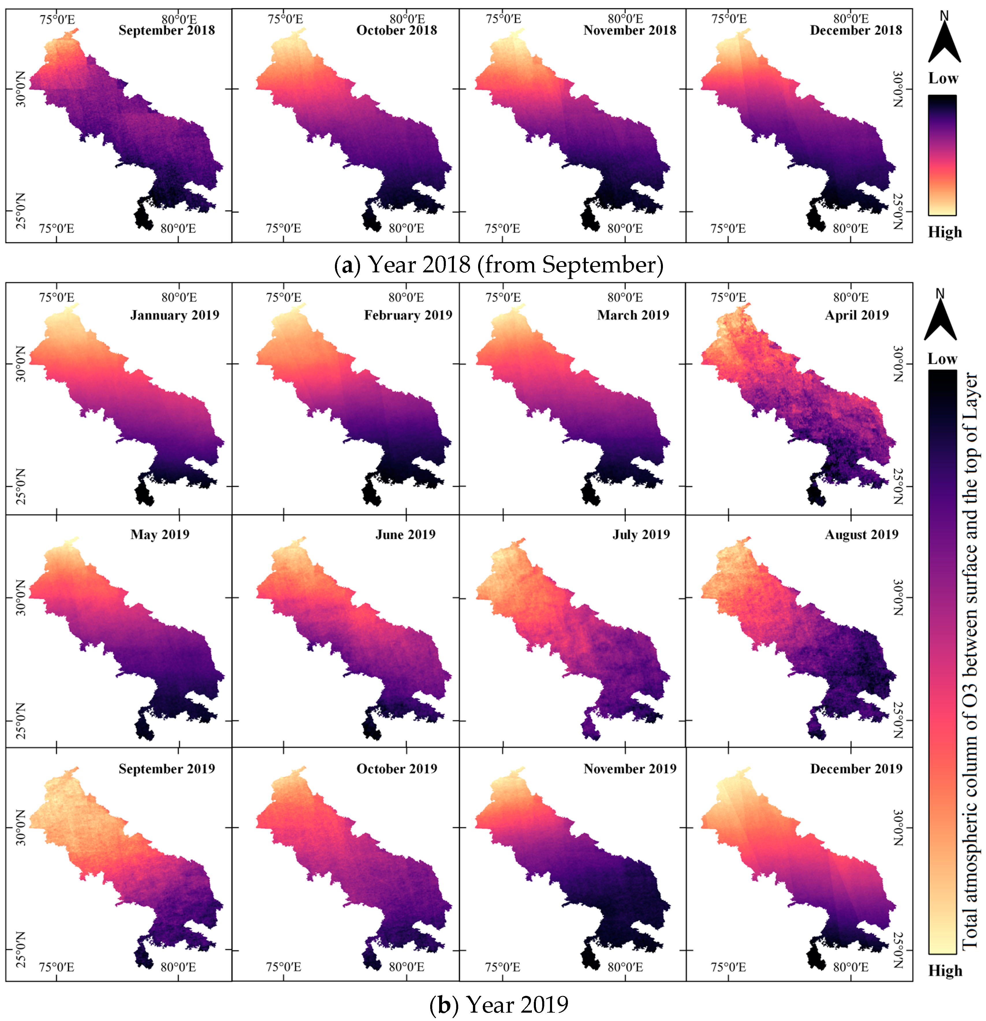
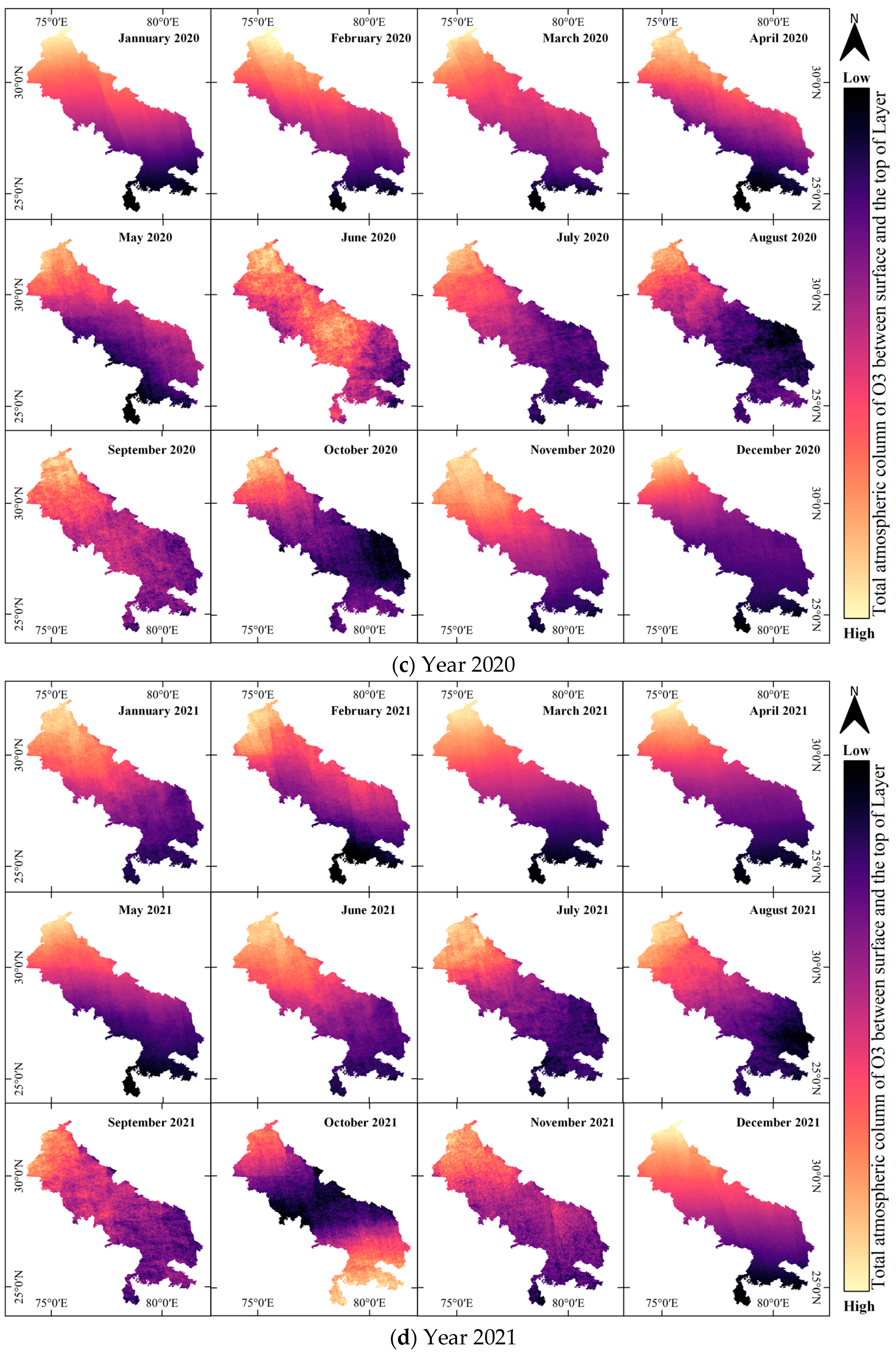
4.3.6. Ozone (O3) Concentration Distribution
O
3 (Ozone) is considered hazardous to organisms when present in the lower troposphere and nearer to ground level. However, it is considered to be beneficial and safe when shielding the biosphere from dangerous solar ultraviolet rays when present in the stratosphere. Tropospheric O
3 is formed by primary pollutants, such as HCHO (see
Section 4.3.7 for brief information). The Sentinel-5P Tropomi is capable of capturing the total atmospheric O
3 concentration with a minimum value of 0.1082 and a maximum of up to 0.1420 mol/m
2. The offline O
3 data from September* 2018 to December 2021 were collected for analysis in the present study (refer to
Table 1 for more information). According to the technical user guides available with the cloud computing engine, the GODfit algorithm is used to calculate the total O
3 for offline products [
49]. Our results showed that the average O
3 concentration is mol/m
2 over the study sites for the chosen time period (refer to
Figure 10). Furthermore, O
3 concentration was found to be highest at 0.1420 mol/m
2 in April 2020, followed by 0.1411 mol/m
2 in April 2021, while the minimum concentration was observed at 0.1080 mol/m
2 in February 2020. The mean Tropospheric O
3 concentrations were found to be 0.1308, 0.1329, and 0.1365 mol/m
2 during the AMJ months for the years 2019, 2020, and 2021 while the mean concentrations were found to be 0.1246, 0.1278, 0.1236, and 0.1280 mol/m
2 in the OND months for the years 2018, 2019, 2020, and 2021.
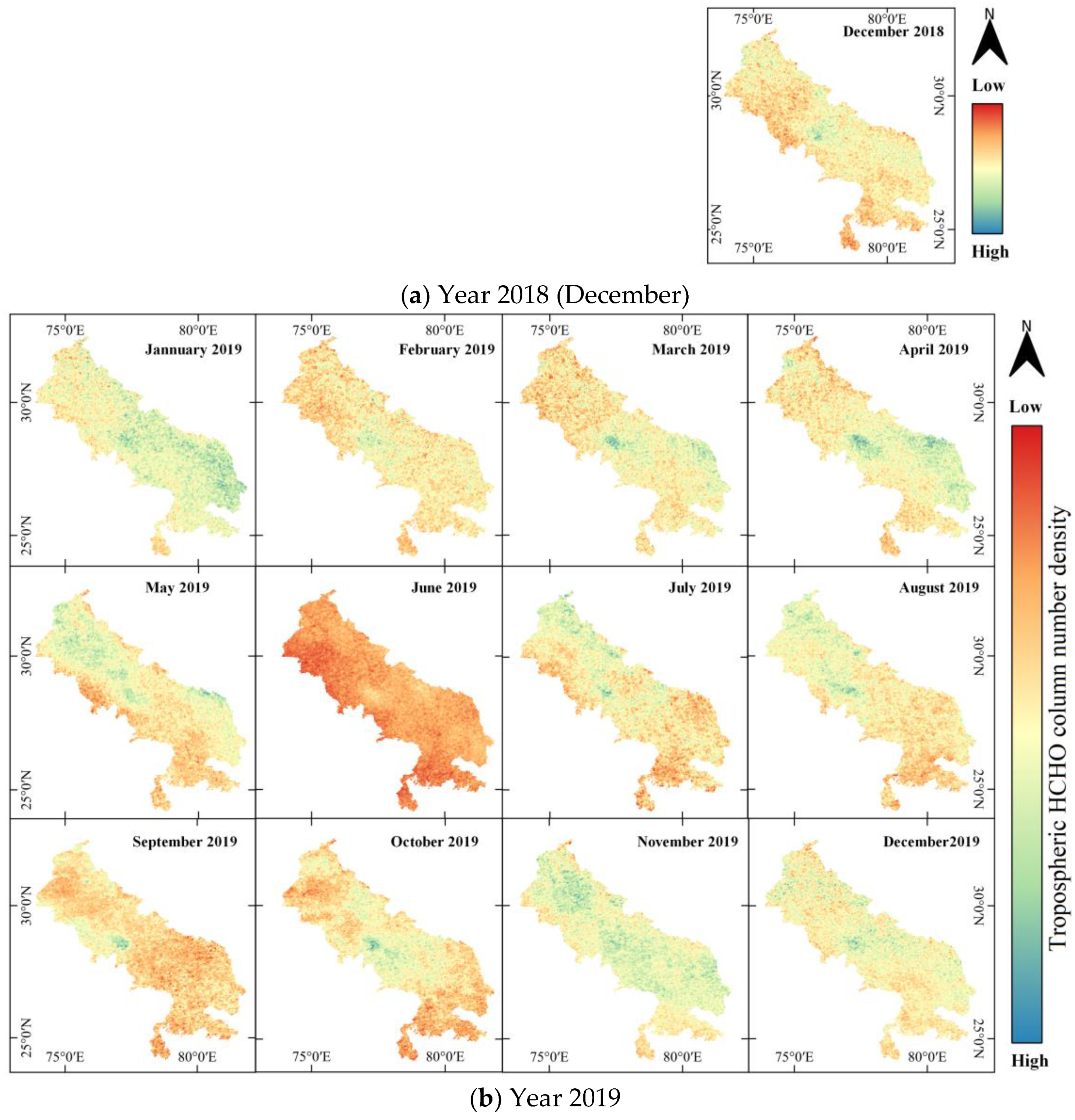
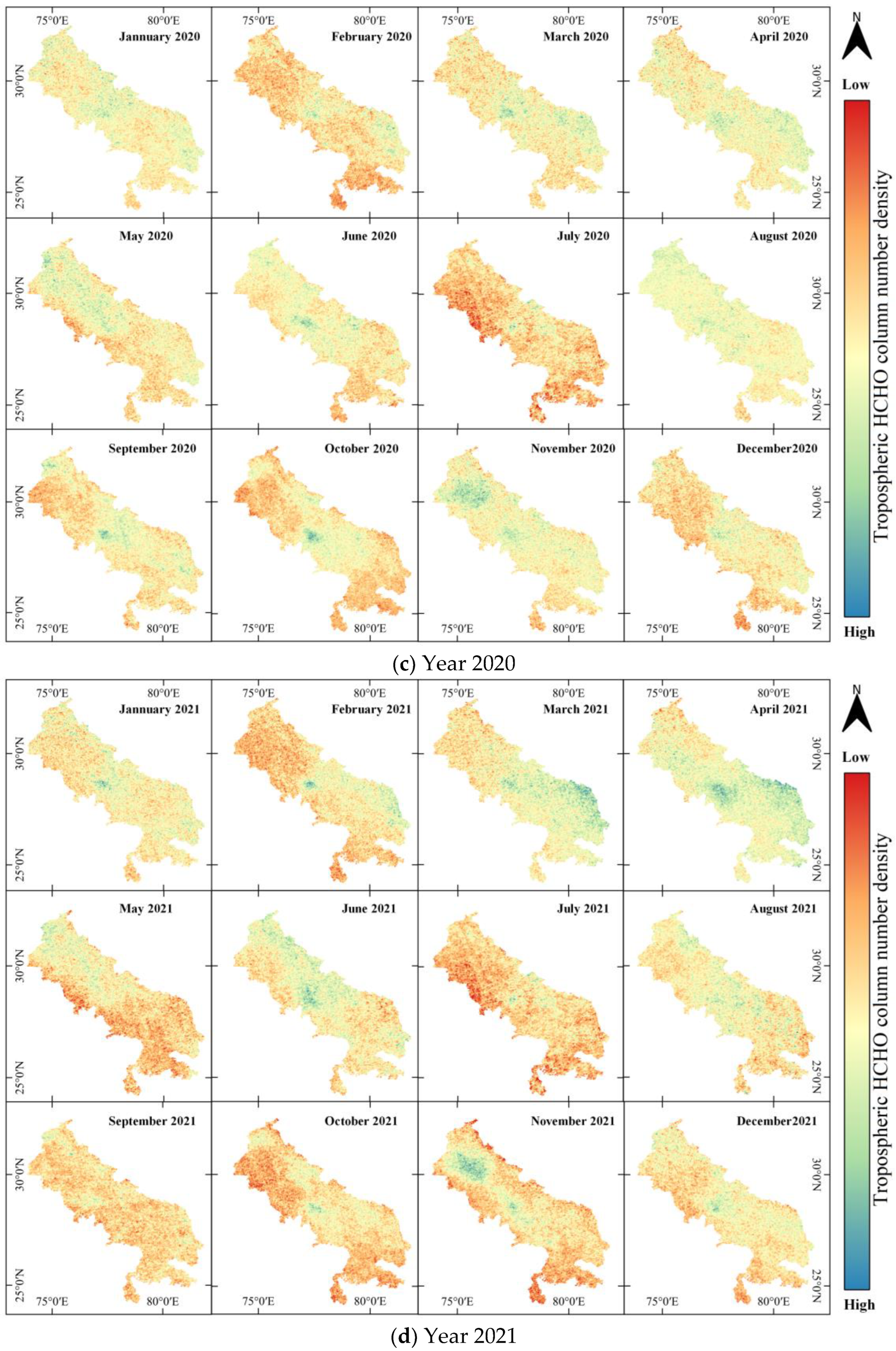
4.3.7. Formaldehyde (HCHO) Concentration Distribution
Formaldehyde (HCHO) is one of the major hazardous air pollutants (HAPs) [
50,
51] among the 187 pollutants (HAPs) that are also known for their carcinogenic effect in outdoor environments [
52]. HCHO is an intermediate gas in almost all oxidation chains of non-methane volatile organic compounds leading eventually to the formation of CO
2 and the concentration of CO
2 in the atmosphere. It also acts as an important precursor to Tropospheric O
3 concentration. These compounds are released into the troposphere by the oxidation of higher non-methane volatile organic compounds emitted mainly from vegetation, fires, and traffic. People are generally exposed to surface concentrations of HCHO, which are directly related to health risks. Detailed information about its hazardous nature and health impact can be found in published works of literature [
50,
51]. Considering the hazardous impact, systematic and accurate ground-based monitoring is difficult and associated with several limitations (expensive, associated errors, small scale-point data) [
53]. Most countries are facing the problem of ground instruments for HCHO sampling, except the USA, which uses a HAPs sampling network, but is limited to urban regions. There is a requirement for the spatio-temporal monitoring of HCHO at different levels, from the local to a global scale [
54]. Therefore, space-borne datasets are suitable for monitoring HCHO and are also supported by Sentinel-5P Tropomi for larger-scale surveillance with effective and accurate outcomes (the maximum achievable value for HCHO concentration was reported to be 0.0074 mol/m
2). Satellite datasets were utilised for mapping HCHO distribution by [
55]. Offline HCHO data from December 2018 to December 2021 were collected for analysis (refer to
Table 1 for more information). According to the technical user guides available with the cloud computing engine, data points whose quality index (QA-value) was less than 0.5 were removed in order to ensure the best quality of output [
56]. Our results show that HCHO’s average concentration is 3.8 × 10
−4 mol/m
2 over the study sites (refer to
Figure 11). The maximum Tropospheric HCHO column number density is found to be 1.31 × 10
−5, 3.72 × 10
−4 and 2.10 × 10
−5 mol/m
2 during the AMJ months for the years 2019, 2020, and 2021 while the concentration is 3.92 × 10
−4, 4.02 × 10
−4, 4 × 10
−4, and 4.6 × 10
−4 mol/m
2 for the OND months of the year 2018, 2019, 2020, and 2021. Furthermore, the HCHO concentration was found to be highest in the southern parts of Haryana, western parts of Punjab, a few parts of Delhi, and the eastern part of UP.
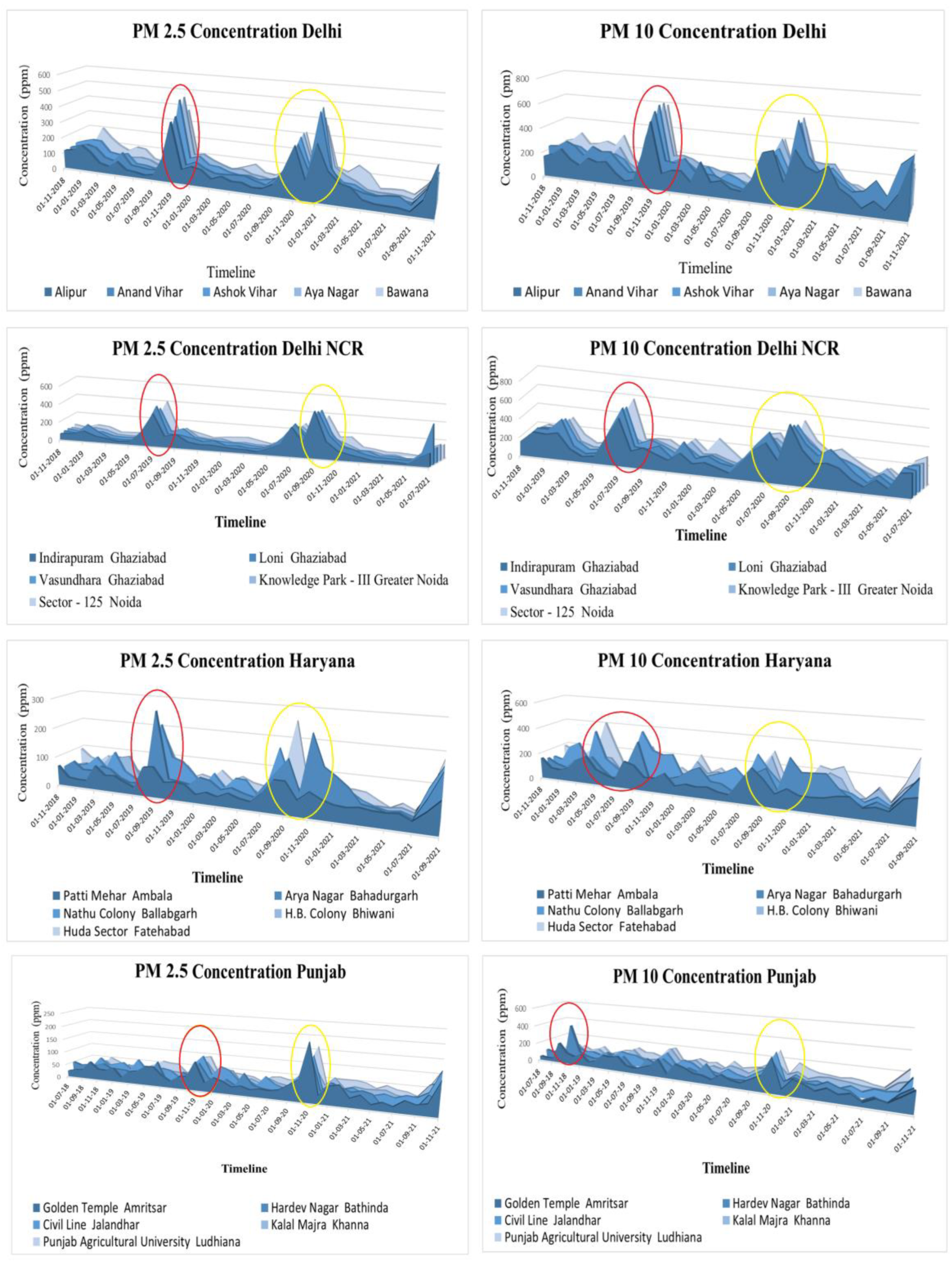
4.4. Ground Station Data for PM2.5/10
Apart from satellite estimation, we have collected the ground samples for the major air pollutants through several agencies, such as the CPCB, for the selected pollutants, PM
2.5 and PM
10.
Figure 12 demonstrates that the concentration is only high in the months following the stubble burning in the vicinity of the states mentioned earlier. In Delhi, the PM emitted by burning stubble is 17 times higher than that emitted by all other sources, including vehicle emissions, the burning of waste, and factories [
57]. The wind speed is the most important parameter that influences the concentration of particulate matter and its transport from the source point to other locations [
58]. Due to the lightweight nature of particulate matter, it floats in the air for a longer time and travels over longer distances; weather conditions amplify the effect of particulate matter by forming smog [
59,
60]. The annual contribution of PM
2.5 and PM
10 is shown in
Figure 11. From the different stations of the study sites, it is clear that the concentration of PM
2.5 and PM
10 is high in the AMJ months and higher in the OND months due to the stable environment. The circles that are highlighted in the graph (refer to
Figure 12) represent the particular time that has been used to demonstrate the PM
2.5 and PM
10 graphs of the Haryana, Punjab, and Delhi areas. It can be concluded that during the AMJ and OND months, the peaks are highest in Haryana and Punjab, as well as some parts of Delhi NCR.
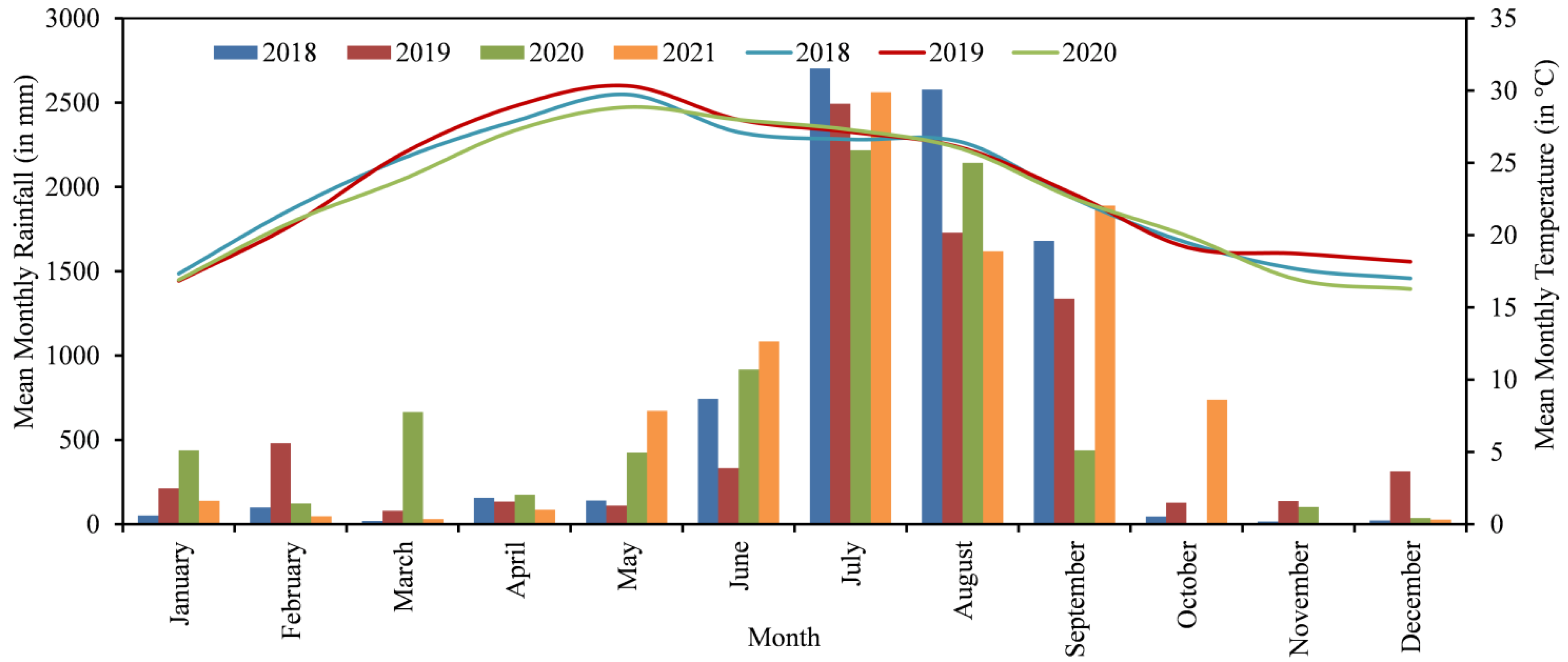
4.5. Rainfall and Temperature Data
Furthermore, rainfall and temperature were considered before inferring from the results. Gridded rainfall (0.25° × 0.25°) and temperature (1° × 1°) from the India Meteorological Department, Govt. of India were utilised to infer the mean monthly rainfall and temperature during the study period [
61,
62]. The temperature data for the year 2021 were not available; therefore, it was not considered in the study. The mean monthly rainfall was relatively low during the AMJ months (April, May, and June) and the OND months (October, November, and December) as compared to the peak monsoon months (July, August, and September). It can be inferred from the rainfall data that after starting July, the amount of rainfall increased, which resulted in a decrease in PM
2.5 and PM
10 concentration (as seen in
Figure 12). The mean monthly temperature is relatively high during April, May, and June (AMJ months) compared to that in the months of October, November, and December for the years 2018, 2019, and 2020 (refer to
Figure 13). It is also inferred that the AMJ months show a relatively higher mean temperature for the years 2018, 2019, and 2020 which probably caused an increase in the concentration of atmospheric pollutants, mainly O
3, and its precursors decreased slightly due to the high temperature and were concerted to secondary pollutants.
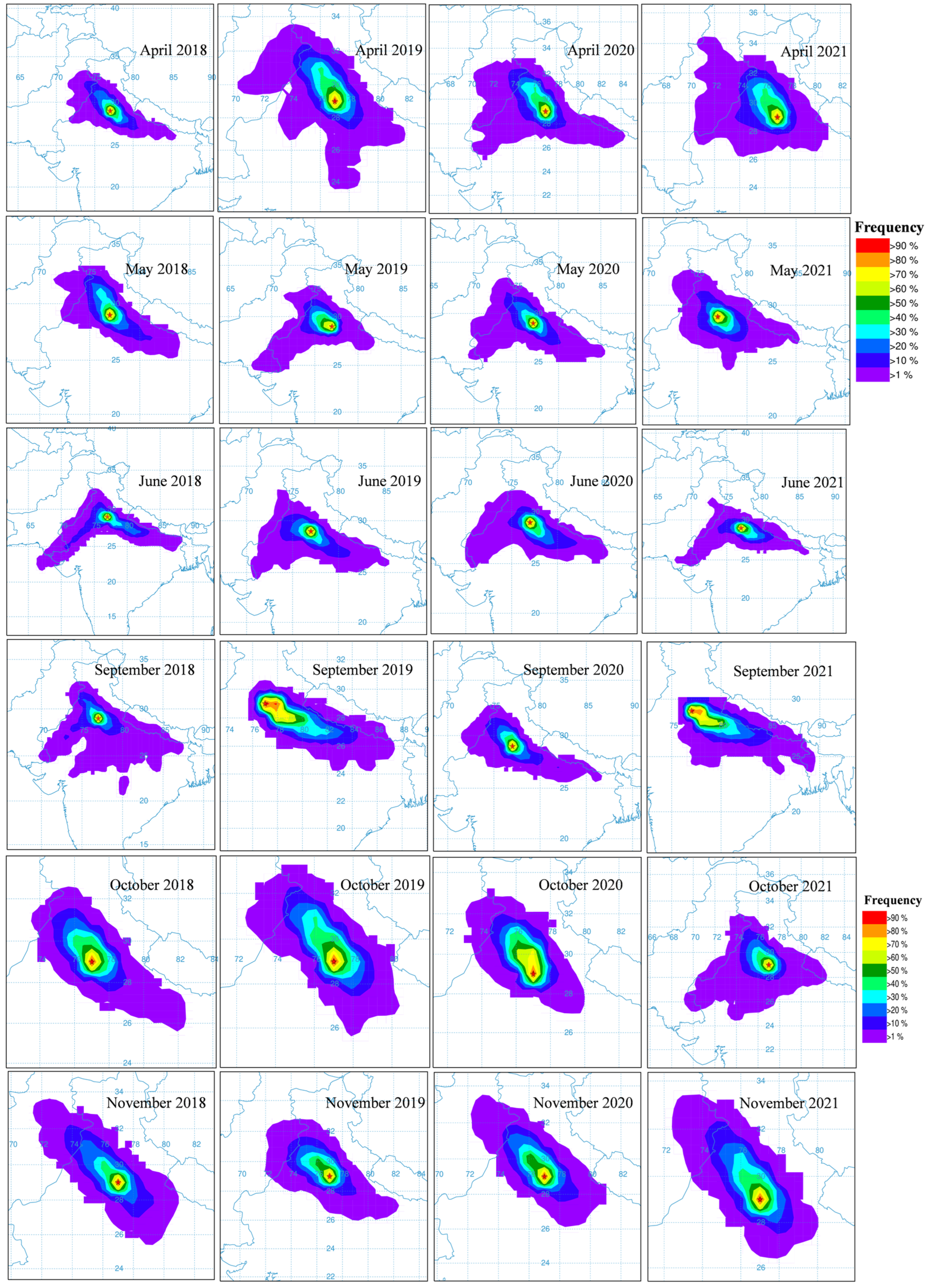
4.6. Trajectory Frequency
The potential medium- and long-range movement of air masses were analyzed using backward trajectories at the defined location for a given time to identify the source region of pollution [
63,
64]. The monthly frequency (April–June and September–December) or backward wind trajectories at all levels in the atmosphere during 2018–2021 were processed using the Global Data Assimilation System (GDAS) meteorological data from the National Centers for Environmental Prediction (NCEP) at a 1° × 1° spatial resolution and the Hybrid Single-Particle Lagrangian-Integrated Trajectory (HYSPLIT) model developed by the National Oceanic and Atmospheric Administration’s Air (NOAA) Air Resources Laboratory (ARL) [
65]. Equation 3 was used to compute the frequency of backward trajectories with no residence time [
65].
The frequency of backward trajectories was analyzed at 77.4508667° E and 28.6568510° N. Trajectory frequency grid resolution and starting time interval was set at 1° × 1° and 6-h, respectively, in the HYSPLIT model.
4.7. Interpretation
The study’s air mass movement comes from the northwest during the pre-monsoon season (April–June) (refer to
Figure 14). During the pre-monsoon season, air masses transport dust and pollutants from Rajasthan, Punjab, and Haryana. In the case of the post-monsoon season, the air masses come from the northwest direction, especially in October and November. In October, the dominant direction of the air mass movement goes from the southeast to the northwest (as seen in
Figure 14). Back trajectory analysis in
Figure 14 indicated that winter air masses reaching Delhi and parts of Uttar Pradesh had travelled long distances during the winter OND months of each year, while during the AMJ months, air masses travelled for a short duration, mainly in the month of June.
5. Conclusions
As demonstrated in the results of the present study, the concentration of pollutants increased after stubble burning from (OND) October to November, followed by from (AMJ) April to June each year. Further, the transboundary pollutants are transported to other states, primarily in the eastern states, from Punjab and Haryana towards New Delhi NCR and Uttar Pradesh. It is evident from the environmental pollutants data retrieved and collected from the CPCB, which confirms the increases in pollutant concentration in the months mentioned above as seen through air mass movements. The higher aerosol concentrations during the AMJ months are interpreted to be a result of the air masses spending more time over land during the summer as compared to winter during the OND months. While monsoonal rainfall tends to reduce aerosol concentrations by removing aerosols and PM2.5/PM10 from the atmosphere, thus causing a decline in their concentration after July and onwards before rising again in the winter season with the renewed stubble burning after Kharif crops have been harvested. Furthermore, several other factors contribute to the aggravated level of atmospheric concentration, such as transportation/vehicular emissions and factory or industrial activities during the winter. These increase the chance of respiratory problems in infants, and older people, with COPD, asthma, bronchitis, and acute respiratory problems, aggravated due to the cold atmospheric climatic conditions.
Environmental conditions, such as wind speed and wind direction, play a significant role in the transportation of transboundary pollution from one place to another through air mass movement, as confirmed in the study (refer to
Figure 13). In this study, we investigated MODIS-derived burned areas and estimated the spatio-temporal density of major atmospheric pollutants (NO
X, SO
x, CH
4, CO, HCHO, aerosols, and O
3) utilizing the Sentinel-5P Tropomi-based analysis for the years from 2018 to December 2021. The results showed a significant increase in CH
4, SO
2, SO
X, CO, and aerosol concentration during the AMJ months (stubble burning of Rabi crops) and in the OND months (stubble burning of Kharif crops) each year. Based on the above discussion, our findings demonstrate that the atmospheric concentration level was highest during the AMJ months as well as in the OND months in the assessment period (November month was the highest level, as confirmed by [
23]. As illustrated in
Figure 3 and
Figure 4 and
Table 2, stubble burning cases were at a maximum during the OND months of each year and burned area assessment using MOD14A1 data also reveal the following trends. The concentration of atmospheric pollutants was also found to be higher during the AMJ/OND months as compared to any other duration in the study site. Our findings from the study reported that all atmospheric pollutants were higher in the OND months (winter season) followed by AMJ months for the years 2018–2021, as seen in
Figure 6,
Figure 7,
Figure 8,
Figure 9 and
Figure 10. The results also support that rice stubble burning generates more emissions, and favourable winter conditions aggregate the concentration over the study regions. A spatio-temporal evaluation of atmospheric pollutants concentration can be used as a basis for evaluating the effectiveness of existing controls, acts, and policies, as well as identifying the alternate solutions to mitigate the problems in the region with a high/increased concentration.
Overall, it can be inferred from the study that Earth observation Sentinel-5P Tropomi based density data provided a significant outcome for the spatio-temporal monitoring of atmospheric pollutants. The outcomes of the present study support the effective monitoring of atmospheric pollutants for their spatio-temporal variations using EO- Sentinel-5P Tropomi. The Sentinel-5 Precursor mission collects data to be utilized for the assessment of air quality, and the monitoring of the concentration of pollutants and is thus considered to be one of the best data sources for atmospheric-pollutant monitoring and distribution for analysis across the globe.


 ,
, 


