Spatial Concept Query Based on Lattice-Tree

Abstract

As a basic method of spatial data operation, spatial keyword query can provide meaningful information to meet user demands by searching spatial textual datasets. How to accurately understand users’ intentions and efficiently retrieve results from spatial textual big data are always the focus of research. Spatial textual big data and their complex correlation between textual features not only enrich the connotation of spatial objects but also bring difficulties to the efficient recognition and retrieval of similar spatial objects. Because there are a lot of many-to-many relationships between massive spatial objects and textual features, most of the existing research results that employ tree-like and table-like structures to index spatial data and textual data are inefficient in retrieving similar spatial objects. In this paper, firstly, we define spatial textual concept (STC) as a group of spatial objects with the same textual keywords in a limited spatial region in order to present the many-to-many relationships between spatial objects and textual features. Then we attempt to introduce the concept lattice model to maintain a group of related STCs and propose a hybrid tree-like spatial index structure, the lattice-tree, for spatial textual big data. Lattice-tree employs R-tree to index the spatial location of objects, and it embeds a concept lattice structure into specific tree nodes to organize the STC set from a large number of textual keywords of objects and their relationships. Based on this, we also propose a novel spatial keyword query, named Top-k spatial concept query (TkSCQ), to answer STC and retrieve similar spatial objects with multiple textual features. The empirical study is carried out on two spatial textual big data sets from Yelp and Amap. Experiments on the lattice-tree verify its feasibility and demonstrate that it is efficient to embed the concept lattice structure into tree nodes of 3 to 5 levels. Experiments on TkSCQ evaluate lattice from results, keywords, data volume, and so on, and two baseline index structures based on IR-tree and Fp-tree, named the inverted-tree and Fpindex-tree, are developed to compare with the lattice-tree on data sets from Yelp and Amap. Experimental results demonstrate that the Lattice-tree has the better retrieval efficiency in most cases, especially in the case of large amounts of data queries, where the retrieval performance of the lattice-tree is much better than the inverted-tree and Fpindex-tree.

1. Introduction

A spatial keyword query (SKQ) is the basic way to meet users’ location-related demands and to explore the huge potential values of spatial textual big data. It is usually used to recommend multiple valuable spatial objects that satisfy location and content requirements to users. With the continuous emergence of massive spatial-temporal big data and the widespread use of LBS (location-based services), SKQ has been extended to a variety of research [1,2,3,4,5] to meet users’ various needs. For example, a spatial group keyword query [6,7,8], spatial keyword skyline query [9,10,11], temporal spatial keyword query [12,13,14], etc. However, the huge data volume and various textual features of spatial textual big data still bring some challenges to the efficiency and effectiveness of SKQ, especially in multi-textual-keywords queries.

Indicating the efficiency of SKQ, most of the existing index structures are evolved from inverted table [1,5,15,16], signature [3,17,18], and bitmap [19], etc. for textual features of spatial data. However, they cannot directly maintain the network-like many-to-many relationships between spatial objects and textual keywords, and multiple complex traversals are required to deal with spatial multi-keywords queries in spatial textual big data. On the other hand, too many textual keywords may often cause trouble for users to set query conditions. Users often only give fuzzy query ideas based on their biased personal experience and knowledge, leading to inaccurate or incomplete results of SKQ [20].

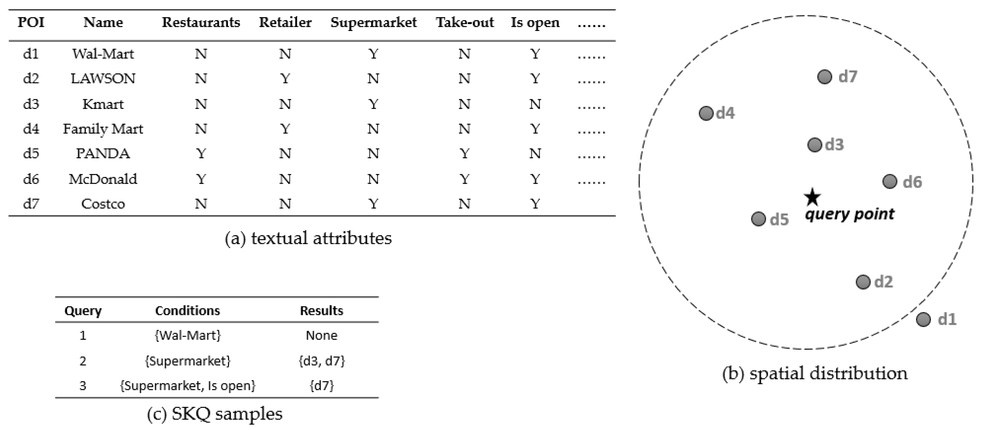
A simple example shown in Figure 1 explains the effect of textual keyword selection on SKQ. In it, seven spatial objects are given, and their textual features and spatial positions are shown in Figure 1a,b. User attempts to find something similar to “Wal-Mart” fall within the limited spatial range, i.e., the dotted circle in Figure 1b. Due to the inadequate understanding of “Wal-Mart” with many textual features in this data context, the conditions of Query 1 and 2 do not accurately characterize “Wal-Mart”. Thus, their query results are incorrect. Only Query 3 finds that “Wal-Mart” is the “open” “supermarket” and “Costco” (d7) is retrieved.

In general, spatial textual big data contain many-dimensional textual features. This data not only enrich the detailed features of spatial objects, but also show the complex associations between spatial objects and offers difficult to efficient SKQ. Most of the traditional SKQ algorithms usually employ spatial location and textual keywords as query conditions to retrieve similar spatial objects in spatial proximity and textual relevancy. However, a lack of knowledge of the textual context often occurs. In this case, users prefer to present their query intention with analogical objects and find similar spatial objects [6,8,9], especially in the condition of many textual features. Therefore, the key to efficient SKQ is to quickly identify similar spatial objects.

To clarify the similarity of spatial objects, we propose a spatial textual concept (STC) to formalize a group of similar spatial objects with several identical textual features in a given spatial range. An STC can be represented by four tuples $\left(r,D,K,I\right)$, $r$ is a spatial region, $D$ is a set of spatial objects, $K$ is a set of textual features, and $I$ is the relationships between $D$ and $K$. We also name the specific SKQ that targets STC as spatial concept query (SCQ) to answer the similar spatial textual objects. In the example shown in Figure 1, $c1=\left(r,s,\left\{supermarket\right\},\left\{d3,d7\right\}\right)$ represents that in the spatial range of $r$, the concept $c1$ contains two objects, d3 and d7. The textual attribute “supermarket” in a spatial region of $s$; and $c2=\left(r,s, \left\{supermarket, Is open\right\},\left\{d7\right\}\right)$ represents that the concept of “open” “supermarket” is $d7$, “Costco”. The many-to-many relationship between spatial objects and textual features can also be presented. More importantly, the users’ real querying intention may be directly identified as the STC $c2$ by the SCQ “Query 3”.

For the maintenance of STCs in spatial textual big data, a novel index scheme and its top-k SCQ algorithms need to be developed. This paper proposes a hybrid index structure, a lattice-tree, by embedding the concept lattice [21] model into the nodes of an R-tree like spatial index structure, in order to construct the STC index structure of spatial textual big data. Concept lattice, proposed by Wille in 1982, is known as a knowledge mining tool, in which concept nodes describe the sets of objects with the same features and the linkages between concept nodes express the hierarchical relationship between them. Due to the many-to-many relationships between objects and features that can be abstracted by concept nodes of a concept lattice directly, the concept lattice model has been employed by some researchers for describing spatial relationships [22], mining spatial association rules [23], and analyzing spatial data warehouses [24], etc. In essence, lattice-tree is still a kind of tree index structure. In it, by embedding concept lattice into tree nodes, STCs within the spatial region of a tree node are indexed by concept nodes of the corresponding concept lattice.

Moreover, this paper also develops the top-k SCQ (TkSCQ) algorithm to efficiently answer STC. The inputs of the TkSCQ algorithm include a spatial range and a spatial object, and the outputs are the top k nearest similar spatial objects belonging to the same STC with the input object. Due to the correspondence between STC and the concept node, efficient TkSCQ can be achieved by traversing tree nodes and concept nodes only once.

To provide accessible and evaluable conclusions, two baseline algorithms based on IR-tree [1,2] and FP-tree [25] are employed, and a series of experiments on performance and efficiency are performed. The experimental results demonstrate the effectiveness and efficiency of the proposed methods.

To sum up, the main contributions are as follows:

(1)

We define spatial textual concept (STC) to formalize a set of similar spatial objects and develop a hybrid index structure, a lattice-tree, to index the STCs in spatial textual big data. By embedding concept lattice structures into R-tree nodes, it can not only supply a tree-like spatial location index but also present the many-to-many relationships between spatial objects and textual features.

(2)

Based on STC, we also develop a top-k spatial concept query (TkSCQ) algorithm to retrieve the set of similar spatial objects from spatial textual big data. The TkSCQ algorithm transforms the user’s query request into an STC and retrieves the similar spatial objects by lattice-tree.

(3)

We conduct a series of performance experiments and comparative experiments with two baseline algorithms. The results demonstrate the applicability of STC to spatial textual big data and the efficiency of the proposed lattice-tree and TkSCQ.

The remainder of this paper is organized as follows. In Section 2, we describe the related work. Section 3 formalizes the model and the problem we are trying to work out. Experimental results are described in Section 4. Finally, we summarize the full paper in Section 5.

2. Related Work

Due to the rapid development of information technology, spatial textual data can be easily accessible and location-based Service has been widely used in various human activities. Some query methods extended from the baseline SKQ method have been proposed. For example, spatial group keyword query [6,7,8], prestige-based SKQ [26], spatial keyword skyline query [9,10,11], level-aware collective SKQ [27], spatial pattern matching [28], social-aware SKQ [29,30,31], etc. Based on the spatial search, these methods pay more attention to the accuracy and efficiency of a textual features query.

With the increase in spatial textual big data, not only its data volume but its structure is becoming more complex, which means that a spatial object has more non-spatial textual features. Although this provides a variety of chances to enrich data applications, it also makes it difficult for efficient retrieval and data mining [32,33]. For this, some efforts hope to identify similar spatial objects with the same textual features to answer SKQ. Spatial group keyword query [6,7,8] tries to find a spatial object group to answer the multi-textual keywords query collectively with the minimum distance cost. Prestige-based SKQ [26] retrieves the most popular objects with the prestige of the given textual conditions. Further, level-aware collective SKQ [27] proposes a level-aware keyword scoring paradigm to ask for a group of similar objects that cover the query keywords collectively. Their query targets are a group of similar spatial objects that meet the query keywords, although their solving process is different.

Motivated by this, we attempt to formalize the group of similar spatial objects with the same textual features as spatial textual concept (STC) and denote its query as spatial concept query (SCQ).

In addition, from the perspective of spatial index structure, most existing spatial index schemes can be considered as a hybrid index structure. They employ tree-like structures, such as R-tree [1,2,17,34,35], Quadtree [3,15], etc., or non-tree structures, such as Grid [5,36], space-filling curve [16,37], etc., to maintain spatial location features. Inverted file [1,5,15,16], Fp-tree [25,38], signature [3,17,18], bitmap [19], etc., are also employed to maintain non-spatial textual features. However, considering a large number of the detailed features of textual features and their many object associations, how to efficiently find and index similar spatial objects from spatial textual big data remains a hot research topic.

Since the textual features of spatial objects are or can be easily transformed into structured data, some classically structured index structures have been widely used to cope with textual keyword retrieval. Some efforts [2,16,35] integrate inverted file-based structure into spatial index structure to answer the single keyword SKQ. They create independent indexes for each keyword and only maintain the one-to-many relationships between textual features and spatial objects. For multi keywords SKQ, multiple rounds of keyword traversal and a large number of set operations are required by an inverted file structure, especially in spatial textual big data [32]. Furthermore, signature based [3] and bitmap based [19] structures can be considered as the extensive version of the inverted file. They only maintain the many-to-many relationships in specific several keywords and a lot of time-consuming set operations are still inevitable to deal with spatial textual big data [33].

In the study of social networks, the many-to-many relationships between social network data are usually indexed by a network structure to maintain the multiplexity [39] and the heterogeneity [40] of social network data, so that social-aware SKQ [29,30,31] can be achieved. Furthermore, to understand the high dimensional textual features, the idea of multi-granularity classification has been applied by S2R-tree [41] and CISK [20] to describe the high dimensional semantic space and the knowledge graph. S2R-tree classifies spatial objects with high-dimensional semantic information according to hierarchy, and CISK classifies similar spatial objects into the concept.

The proposed spatial textual concept also inherits the idea of classification to model the many-to-many relationships between objects and features. Based on the concept lattice structure, the proposed spatial concept query for STC can retrieve similar spatial objects directly.

A concept lattice [21] is a lattice structure that represents the hierarchical relationships between concepts. Each of its nodes is a concept that includes some objects with the same features. It has been widely used in information retrieval [42], knowledge discovery [43], association analysis [44], recommender systems [45], and software engineering [46]. Obviously, concept lattice is a perfect carrier for the STC to carry the many-to-many relationships in spatial textual big data.

Therefore, this paper hopes to introduce the concept lattice model to maintain STC and proposes a novel hybrid index structure, a lattice-tree, to explore the manipulating mechanism of spatial object similarity. By embedding a concept lattice into some nodes of the R-tree index, the lattice-tree integrates spatial and textual information into STC in a seamless way, and all many-to-many relationships in a tree node are fully presented as the concepts of concept lattice structure [43]. Instead of indexing spatial objects, the lattice-tree takes STC as the index object so that the efficient query for STC can be achieved. The Top-k spatial concept query (TkSCQ) algorithm is developed to retrieve the k nearest to similar spatial objects in an STC. Theoretically, due to the full coverage of a concept lattice to STC [44], the lattice-tree can find all valuable relationships in spatial textual big data and is conducive to accurately understanding the query intentions.

3. Methodology

3.1. Principles

As a new way to explore the complex relationships between spatial objects, the proposed spatial textual concept STC is used to present a group of similar spatial objects with the same textual features within a certain spatial region. In this section, a series of formal definitions of STC are presented, and the index structure Lattice-tree and the retrieval scheme Top-k spatial concept query (TkSCQ) for STC are proposed.

Lattice-tree is a hybrid index structure including a tree index structure and some concept lattice structures. It employs an R-tree structure to maintain the spatial information of objects and embeds a concept lattice structure into a tree node to organize the textual information of objects in the tree node as STCs. The concept lattice structure is the complete set of the many-to-many relationships and its volume is proportional to the quantity and complexity of textual features, so only some tree nodes that contain a moderate number of objects contain a concept lattice. TkSCQ is a proposed STC retrieval algorithm based on lattice-tree for spatial textual big data. By traversing the lattice-tree, it can accurately retrieve STCs that meet the query conditions to explore the many-to-many relationships between similar spatial objects.

3.2. STC Formulations

Spatial Textual Big Data can be denoted as a set of spatial objects, $\mathbb{D}=\langle {\mathit{d}}_{\mathit{i}}=\left\{\mathit{p},\mathit{K}\right\},\mathit{p}\in \mathit{P}, \mathit{K}\subseteq \mathbb{K}\rangle$, where $d_i$ is the $i$th spatial object with the spatial information $p$ and a textual feature set $\mathit{K}=\langle k_1,k_2,\dots ,k_j\rangle$. $\mathbb{K}$ represents the full set of textual features. $K$ represents the set of possible features that a location $\mathit{p}$ can have or not, which is the subset of $\mathbb{K}$, $\mathit{K}\subseteq \mathbb{K}$. $\mathit{P}$ represents the set of all the locations $p$. For example, the “Wal-Mart” in Figure 1 can be represented by $d_1=\{p_1,\left\{supermarkey, is\_open\right\}$ Spatial Textual Concept (STC) represents a set of spatial objects $D$ and their common textual features $K$ within a considered spatial region $r$. An STC $\mathit{c}$ can be defined by a tuple, $\mathit{c}=\left\{\mathit{r},\mathit{D},\mathit{K},\mathit{I}\right\}$, where

• $\mathit{r}$ is the considered spatial region,
• $\mathit{D}\subseteq \mathbb{D}$, is a set of spatial objects contained in $\mathit{r}$,
• $\mathit{K}\subseteq \mathbb{K}$ represents the common features of the spatial object of $\mathit{D}$.
• $\mathit{I}\in \mathit{D}\times \mathit{K}$ represents the pairs $\left(d,k\right)$ indicating that the spatial object $d$ in $\mathit{D}$ has the feature $k$ in $\mathit{K}$.

In addition, to present the many-to-many relationships between spatial objects and textual features in an STC, two operators, $f$ and $g$, are defined below.

$$f\left(D\right)=\{k\subseteq K|\forall d\subseteq D, \left(d,k\right)\in I\}$$

$$g\left(K\right)=\{d\subseteq D|\forall k\subseteq K, \left(d,k\right)\in I\}$$

The $f$ operation represents that each spatial object $d$ of $D$ has the textual features $K$, and the $g$ operation represents that each textual attribute $k$ of $K$ belongs to the object set $D$. Then an STC $c$ must satisfy the following constraints: $f\left(c.D\right)=c.K$ and $g\left(c.K\right)=c.D$.

Concept Lattice can be used to represent the hierarchical relationship between STCs. Given two STC $c_1=\left(r,D_1,K_1\right)$ and $c_2=\left(r,D_2,K_2\right)$ covering the same spatial region $r$, the following partial order relation is defined as:

$$c_1\le c_2\iff D_1\subseteq D_2\left(\iff K_2\subseteq K_1\right)$$

And $c_1$ is called the sub-concept of $c_2$, $c_2$ is called the super-concept of $c_1$. Based on this, the Concept Lattice $\mathit{L}$ considering the set $\mathit{C}$ of STCs existing in the spatial region $r$, can be formally defined as follows

$$\mathit{L}=\left\{\mathit{r},\mathit{C},\le \right\}$$

where $\le$ is the partial order relation defined above.

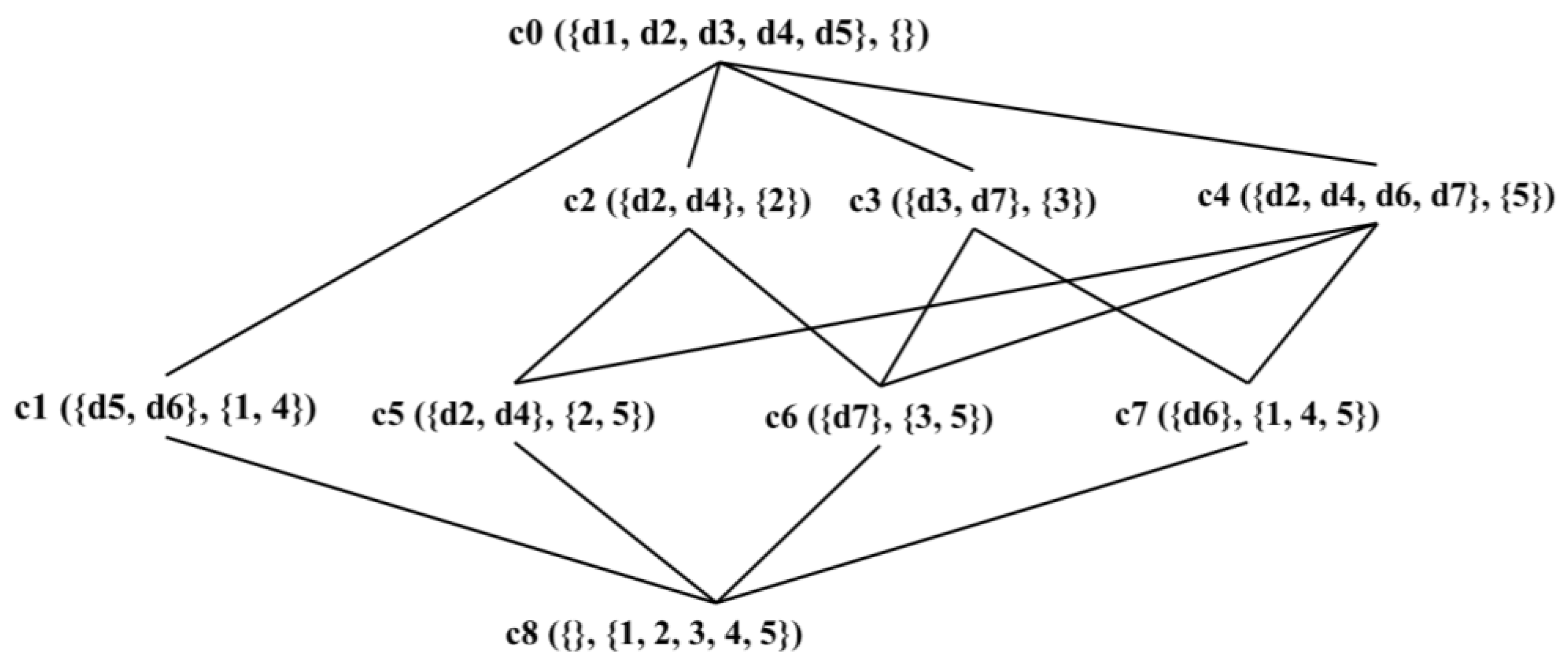
To demonstrate the concept lattice, an example employing the case data in Figure 1 is shown in

Table 1. The STCs of Example.

STC	Extent	Intent *
c0	d2, d3, d4, d5, d6, d7	$\varnothing$
c1	d5, d6	1, 4
c2	d2, d4	2
c3	d3, d7	3
c4	d2, d4, d6, d7	5
c5	d2, d4	2, 5
c6	d7	3, 5
c7	d6	1, 4, 5
c8	$\varnothing$	1, 2, 3, 4, 5

* 1: Restaurants, 2: Retailer, 3: Supermarket, 4: Take-out, 5: Is open.

and Figure 2. For the sake of readability, in Figure 2, each STC $\left\{r,D,K,I\right\}$ reported in the nodes of the lattice is represented only by listing the set of objects $D$ and the common features $K$. The search region can be understood as the area that meets the query conditions of TkSCQ (see details for Section 3.3). Because the spatial object $d_1$ is out of the search region, it is ignored and the objects $d_2$ to $d_7$ need to be considered. Table 1 shows the 9 STCs from $d_2$ to $d_7$: $c_0$ is the top STC, and $c_8$ is the bottom concept. The corresponding concept lattice structure is shown in Figure 2.

3.3. Lattice-Tree

Lattice-tree is the proposed hybrid index structure. Its main idea is to embed concept lattice structure into nodes of the R-tree to maintain STC. Similar to R-tree [47], the lattice-tree also employs the minimum bounding rectangle (MBR) to split spatial regions and build a tree index structure to index the spatial information of spatial objects. For the textual features of spatial objects, the lattice-tree inserts a concept lattice structure into some tree nodes. Then the spatial information and textual features of spatial objects can be integrated into tree nodes in a seamless way.

Let $\mathbb{T}=\left\{\langle {\mathit{n}}_{\mathit{i}}\rangle ,\mathit{\delta },\mathit{𝓇}\right\}$ be a Lattice-tree, where $\langle n_i\rangle$ is the set of tree nodes, and $n_i=\left\{id,pn, cns, level,mbr, L\right\}$ is the tree node structure containing the id of node, $id$; parent node, $pn$; and children nodes, $cns$; the level of node in tree, $level$ (the $level$ of leaf node is 0, and the $level$ of tree root is the maximum value); the minimum bounding rectangle, $mbr$; and the concept lattice structure, $L$. $\delta =\left[{\delta }_{min},{\delta }_{max}\right]$ is the range of the tree node’s entries, i.e., the number of child nodes of the tree node, and $𝓇=\left[{𝓇}_{min},{𝓇}_{max}\right]$ is the threshold for the $level$ of tree node, that determines whether the tree node contains the concept lattice structure.

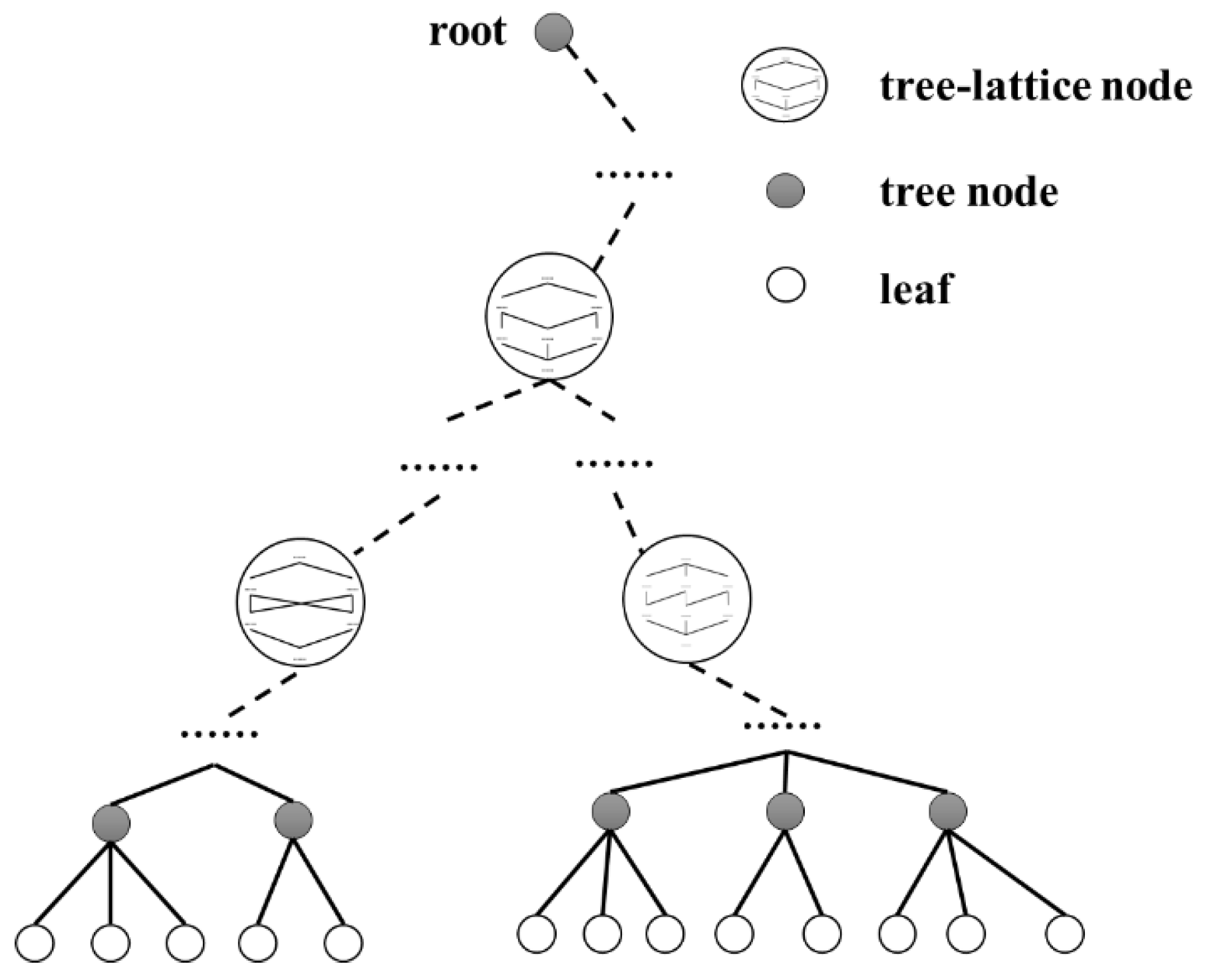
As shown in Figure 3, there are three kinds of tree nodes in the lattice-tree. When the $level$ of a tree node is in the range of $𝓇$, the tree node, named tree-lattice node, contains a $L$ structure, else the tree node only indexes the raw data of spatial objects. The reason for this is that the concept lattice is the complete set of STC, and too much data will make the concept lattice bloated and inefficient. Therefore, we hope to only embed the concept lattice on some tree nodes with a smaller data volume and a larger $level$ to achieve good performance. The detailed evaluation of this is shown in Section 4.2.

The initialization process of the lattice-tree is shown in Algorithm 1. It is a progressive algorithm that can insert spatial objects into the lattice-tree one by one by traversing the spatial textual big data set once.

Its inputs are the spatial textual big data set $\mathbb{D}$, the parameter of the tree node entries, $\delta$, and the concept lattice building parameter, $𝓇$. Its output is the Lattice-tree index structure $\mathbb{T}$. The initialization process consists of two steps. First, in lines 1 to 6, incrementally create the tree structure based on the spatial information of spatial objects. Similar to the classical initialization algorithm of R-tree [47], Algorithm 1 creates a tree structure of $\mathbb{T}$ by inserting spatial objects $d$ into a tree node whose MBR covers $d$. Then, in lines 7 to 13, it generates STCs and creates a concept lattice structure $L$ in a tree node $n$ whose $level$ is in $𝓇$. The construction process of the concept lattice is referenced from [21] but is not described in this article.

In addition, the update process of the lattice-tree is similar to Algorithm 1. Insert some new spatial textual objects into the tree nodes and update the tree structure by updating the algorithm of R-tree. Then, traverse the tree-lattice nodes and insert new objects into the concept lattice structure by the process detailed in lines 6 to 10 in Algorithm 1.

Algorithm 1: The initialization of lattice-tree

Input: $\mathbb{D}$, $\delta$, $𝓇$; Output: $\mathbb{T}$;  1: for each $d\in \mathbb{D}$: //create tree structure  2:  insert $\mathrm{d}$ into $\mathbb{T}.\mathrm{n}$;  3:  if $\mathbb{T}.n.cns>\delta$:  4:   generate a new tree node $n^{\prime }$ and update $\mathbb{T}$;  5: end for;  6: for each $n\in \mathbb{T}$: //create concept lattice structure  7:  if $n.level\mathrm{in}𝓇$:  8:   generate the STC set of $n$ → $C$;  9:   $L=\left(n.mbr,C,\le \right)$ 10:   $n\leftarrow L$ 11: end for 12: return $\mathbb{T}$

3.4. Top-k Spatial Concept Query

SCQ can be considered as an improved version of the basic SKQ (spatial keywords query). It does not match spatial objects one by one according to the user’s query conditions but conducts conceptual inference from a target object by matching STC, and returns a set of similar spatial objects. It is conducive to the query condition selection and the integrity of query results under the condition of many textual features.

A Top-k spatial concept query (TkSKQ) is represented by $q=\left(k,p,\widehat{d}\right)$, where $k$ is the expected number of query results, $p$ is the spatial location of the querier, and $\widehat{d}$ is the target spatial object. The query returns a set $\widehat{D}$ of $k$ spatial objects similar to $\widehat{d}$ and $\widehat{D}\subset \mathbb{D}$, such that (1) $\left|\mathcal{D}\right|=k$; (2) $\forall d\in \mathcal{D}$, $d$ and $\widehat{d}$ belong to the same STC; (3) $\forall d\in \mathcal{D}$, $A\subseteq d.K$, and $\forall d^{\prime }\notin \mathcal{D}$, $A\subseteq d^{\prime }.K$; then $dist\left(d,p\right)<dist\left(d^{\prime },p\right)$.

In Figure 1 and Figure 2, in the number of query results, $k$, is 1, $p$ is the query point identified by asterisks in Figure 1b, and $\widehat{d}$ is the expected object. The TkSKQ of “Wal-Mart” can be represented as $q=\left(1,“query point”,“\mathrm{Wal}-\mathrm{Mart}”\right)$. To achieve this, we firstly retrieve the textual features of “Wal-Mart” from the lattice-tree, i.e., {Supermarket, Is open}, and find the tree-lattice nodes with a smaller MBR, i.e., a larger level, from the lattice-tree, then we retrieve the concept lattice structure to achieve $k$ ($k$ = 1) object belonging to the same STC as “Wal-Mart”, i.e., d7.

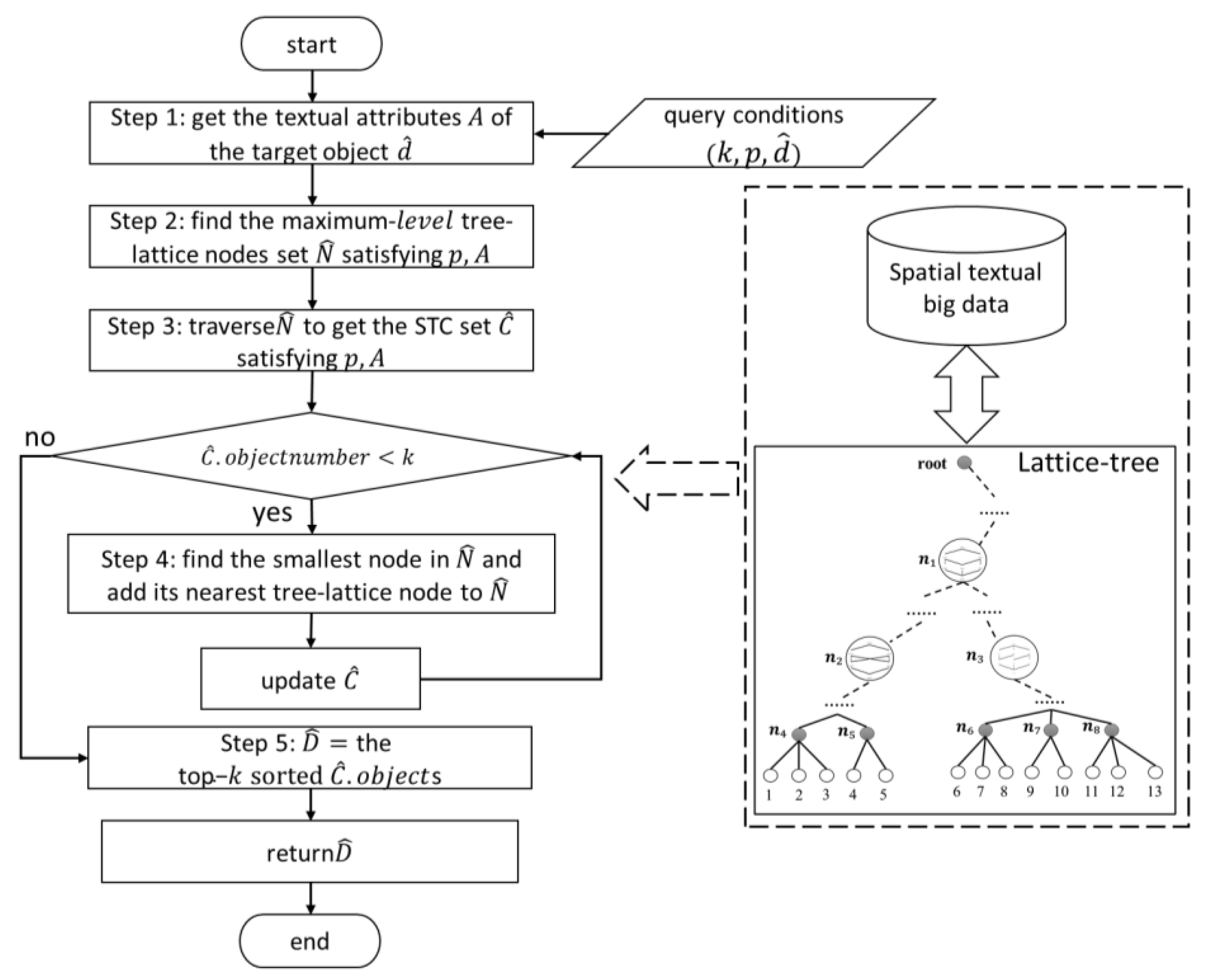
The flow chart of the TkSCQ algorithm is shown in Figure 4. It consists of five steps. Step 1 infers query conditions based on query inputs. Since many textual features will bring trouble to the accurate selection of query parameters, as in the query example in Figure 1, query inputs are often incomplete or inaccurate. Therefore, TkSCQ takes a target spatial object as one of the query inputs, retrieves its textual features $A$, and transforms the query conditions $\left(k,p,\widehat{d}\right)$ to $\left(k,p,A\right)$. Step 2 traverses the lattice-tree to find the tree-lattice nodes set $\widehat{N}$ with the maximum $level$ and $p$, $A$. Step 3 obtains the STCs set $\widehat{C}$ from $\widehat{N}$. If the number of spatial objects in $\widehat{C}$ is less than $k$, Step 4 replaces the “smallest” tree-lattice node with its “nearest” tree-lattice node. The “smallest” mean, the least number of spatial objects and the “nearest” means the nearest tree-lattice node along the lattice-tree structure. Otherwise, Step 5 retrieves and sorts all spatial objects in $\widehat{C}$ from the lattice-tree as $\widehat{D}$ and returns $\widehat{D}$ the results of TkSCQ.

Algorithm 2 presents the main details of the proposed TkSCQ. Its inputs are the expected number of query result $k$, the spatial location $p$, the target spatial object $\widehat{d}$, and the Lattice-tree index structure $\mathbb{T}$. Its output is the set of $k$ sorted spatial objects $\widehat{D}$. Corresponding to the process of the flowchart shown in Figure 4, the implementation of each step is described. In Step 1, in line 1, the textual features of the target spatial object $\widehat{d}$ are retrieved by traversing the tree nodes of $\mathbb{T}$. Step 2, in lines 2 to 8, retrieves the tree-lattice nodes with $level=\mathbb{T}.{𝓇}_{max}$, the spatial location $p$, and the textual features set $A$. Step 3, in lines 9 to 12, traverses the concept lattice structure of each node in $\widehat{N}$ to retrieve the STCs set $\widehat{C}$. Step 4, in lines 13 to 18, judges whether the number of spatial objects in $\widehat{C}$ meet $k$. If not, retrieve the tree node with the least number of objects and add its nearest tree-lattice node to $\widehat{N}$ and update $\widehat{C}$. Step 5, in lines 19 to 20, sorts the spatial objects in all STCs of $\widehat{C}$ by the distance from $p$ and finds the k spatial objects $\widehat{D}$ to $p$. Finally, it returns $\widehat{D}$.

Because the two main components, the R-tree structure and concept lattice structure of the Lattice-tree have the logarithmic retrieval efficiency [21,47], the time complexity of traversing objects from the lattice-tree can be considered as $O\left(nlogn\right)$. In addition, Step 1 and 2 of Algorithm 2 traverses the tree structure and lattice structure with $O\left(nlogn\right)$, Step 3 traverses some lattice structures with $O\left(nlogn\right)$, and Steps 4 and 5 traverse objects in concept lattice structures with $O\left(n^2\right)$. Therefore, we think that the time complexity of Algorithm 2 is $O\left(nlogn+n^2\right)$.

Algorithm 2: TkSCQ

Input:$k,p,\widehat{d},\mathbb{T}$; Output: the set of $k$ sorted spatial objects $\widehat{D}$;  1: traverse $\mathbb{T}$ to retrieve the spatial object $\widehat{d}$ and let $A=\widehat{d}.K$; //Step 1  2: $t\leftarrow \mathbb{T}.root$   //Step 2  3: while $t\ne \varnothing$:  4:   if $t\left[0\right].level=\mathbb{T}.{𝓇}_{max}$ and $\exists c\in t\left[0\right].L.C$, $c.K=A$:  5:    $\widehat{N}\leftarrow t\left[0\right]$  6:  if $p in t\left[0\right].child.mbr$:  7:   $t\leftarrow t\left[0\right].child$ and delete $t\left[0\right]$ from $t$  8: end while  9: for each $n\in \widehat{N}$: //Step 3 10:  if $\forall c\in n.L.C$, $c.K=A$ 11:   $\widehat{C}\leftarrow c$; 12: end for 13: while $\widehat{C}.objectnumber<k$: //Step 4 14:  $n^{\prime }$ = min ($\widehat{N}$); 15:  $n^{″}$ = the nearest tree-lattice node of $n^{\prime }$; 16:  insert $n^{″}$ into $\widehat{N}$; 17:   update $\widehat{C}$; 18: end while 19: $S=\mathrm{sort}\left(\widehat{C}.objects\right)$ //Step 5 20: $\hat{D}=S[0:k]$ 21: return $\widehat{D}$

4. Experiment

In this section, we conduct extensive experiments to evaluate the performance of the proposed lattice-tree and TkSCQ algorithm on a real dataset. All of the experiments were deployed on a computer with intel core i5, 3.0 GHz CPU, 24GB RAM, and 64-bit Windows 10, and all the experimental code were written in python 3.7 and several popular libraries, e.g., NumPy, pandas, etc. The experimental data, code and results have been published in https://gitee.com/xapGitee/lattice-tree.git (accessed on 17 April 2022).

4.1. Data and Preprocessing

To evaluate the effectiveness of the proposed methods, two examples of STDB, yelp and amap, are employed. The yelp dataset used in this paper comes from yelp.com, the most popular review site in the United States, which provides a typical spatial textual dataset “business” containing 192,690 spatial objects with the 12 fields in the United States. This paper employs the “business” dataset as the spatial textual big data to evaluate the lattice-tree and the TkSCQ. The other is a POI (point of interest) dataset from amap.com, named “amap”, which contains 483,990 business POIs in Shanghai, China.

To model the spatial objects of the yelp dataset, some fields are extracted from “business”. The fields of “latitude” and “longitude” are employed to the spatial information, and these 5 fields: “stars”, “review_count”, “Is_open”, “categories”, and “attributes” are transformed into 45 binary textual features. They are 3 textual features: S_low, S_middle, S_high from “stars”; 3 features, S_low, S_middle, S_high from “review_count”; 1 attribute Is_open from “Is_open”; 26 features, Beauty & Spas, Education, Health & Medical, Automotive, Bars, Mass Media, Event Planning & Services, Financial Services, Local Services, Local Flavor, Gyms, Parks, Home Services, Fitness & Instruction, Pets, Shopping, Religious Organizations, Active Life, Landscape Architects, Public Services & Government, Restaurants, Hotels & Travel, Professional Services, Arts & Entertainment, Nightlife, Food from “categories”; and 8 features, Alcohol, DogsAllowed, GoodForDancing, HasTV, Music, Open24Hours, Smoking, WIFI, RestaurantsTableService, GoodForKids, GoodForGroups, AgesAllowed from “attributes”. Then, the spatial textual big data ${\mathbb{D}}_{yelp}=\langle d_i=\left\{p,K\right\},K\subseteq {\mathbb{K}}_{yelp}, 0\le i\le 192690\rangle$, and ${\mathbb{K}}_{yelp}=\left\{k_j\right|j\le 45\}$.

amap only has location information and a few textual keywords. To ensure the diversity of experimental scenes and the comparability of experimental results, we redesign 30 simulation textual keywords similar to yelp to expand amap. Then, the data volume of amap with 483,990 spatial objects is greater than that of yelp with 192,690 spatial objects, and the data complexity of amap with 30 textual keywords is lower than that of yelp 45 keywords. ${\mathbb{D}}_{amap}=\langle d_i=\left\{p,K\right\},K\subseteq {\mathbb{K}}_{amap}, 0\le i\le 483990\rangle$, and ${\mathbb{K}}_{amap}=\left\{k_j\right|j\le 30\}$.

${\mathbb{D}}_{yelp}$ has higher textual complexity (more keywords) and less data than ${\mathbb{D}}_{amap}$, and the indexing mechanism of the lattice-tree can be explored comprehensively by employing them.

4.2. The Initialization of Lattice-Tree

In the lattice-tree index structure, 2 parameters $\delta$ and $𝓇$ need to be considered for its initialization. According to the existing mature schemes [1,2,17,34,35], the number of tree node entries $\delta$ is often taken as [2,4]. Therefore, in this paper, Lattice-tree still uses this setting $\delta =\left[2,4\right]$. By it, the Lattice-tree ${\mathbb{T}}_{yelp}$ of ${\mathbb{D}}_{yelp}$ contains 291,678 tree nodes (192,609 leaf nodes and 99,069 non-leaf nodes) in 12 level, and the Lattice-tree ${\mathbb{T}}_{amap}$ of ${\mathbb{D}}_{amap}$ contains 732,340 tree nodes (483,990 leaf nodes and 248350 non-leaf nodes) in 14 level. Their leaf nodes are on level 0, and the descriptive statistics of tree nodes in Lattice-tree are shown in

Table 2. The descriptive statistics of ${\mathbb{T}}_{yelp}$ and ${\mathbb{T}}_{amap}$.

Description	${\mathbb{T}}_{\mathit{y}\mathit{e}\mathit{l}\mathit{p}}$	${\mathbb{T}}_{\mathit{a}\mathit{m}\mathit{a}\mathit{p}}$
Data volume	100 Mb	192 Mb
Index volume	487 Mb	1193 Mb
The number of objects	192,690	483,990
The number of features	45	30
Total of level	12	14
The number of leaf nodes	192,690	483,990
The number of non-leaf nodes	99,069	248,350

.

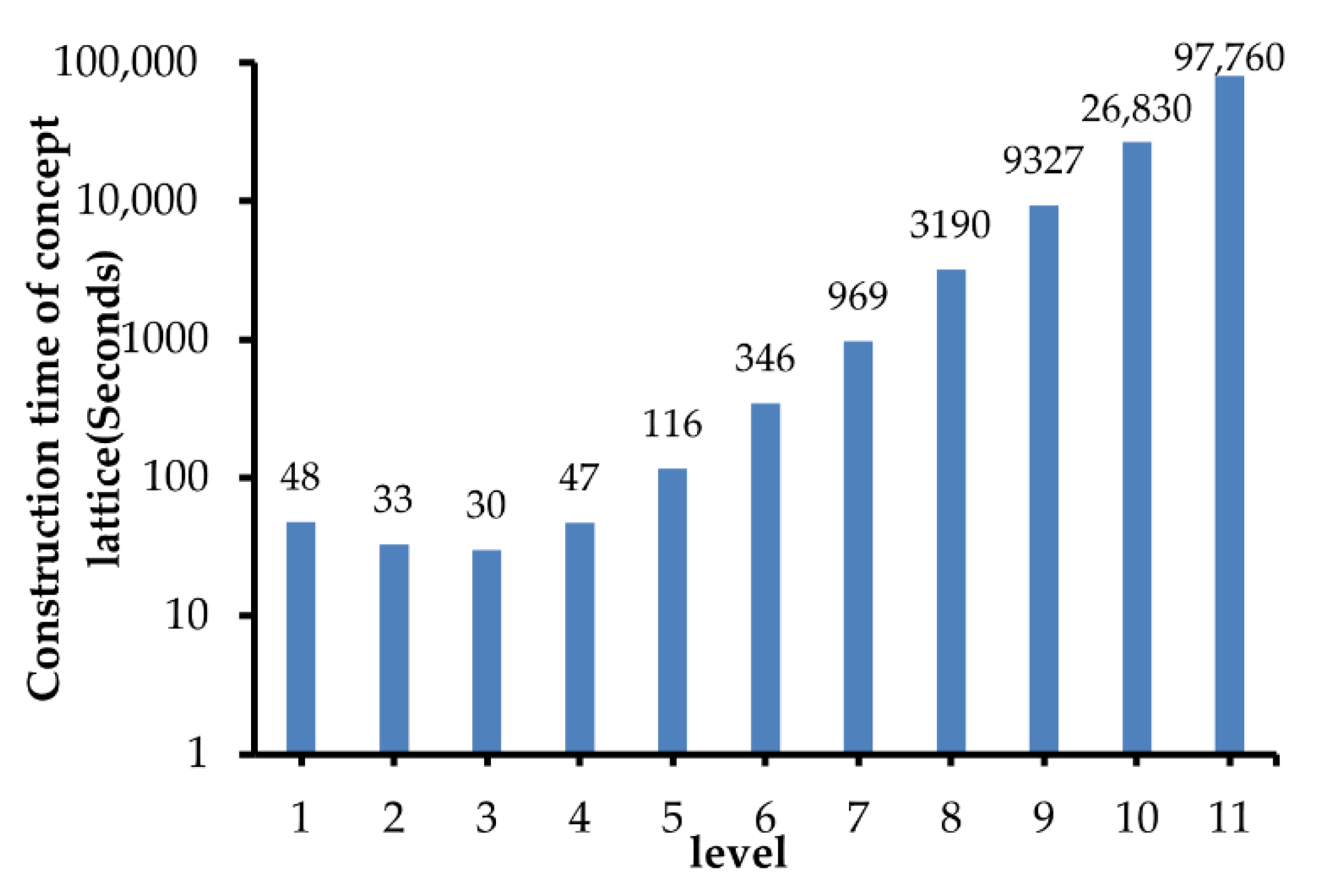
Another parameter $𝓇$ is related to the level of tree node and it determines on which level the tree-lattice nodes should be created. For evaluating the effective of $𝓇$, the time consumptions of constructing tree-lattice nodes in each level are measured and shown in Figure 5. Obviously, the initialized time of a tree-lattice node is positively related to the number of spatial objects it contains, and the performances of level 1 to 5 are better than others. In addition, too few objects in a tree-lattice node are not conducive to the expression and retrieval of the complex relationships between objects, and these nodes in level 1 to 2 are not suitable as the tree-lattice node.

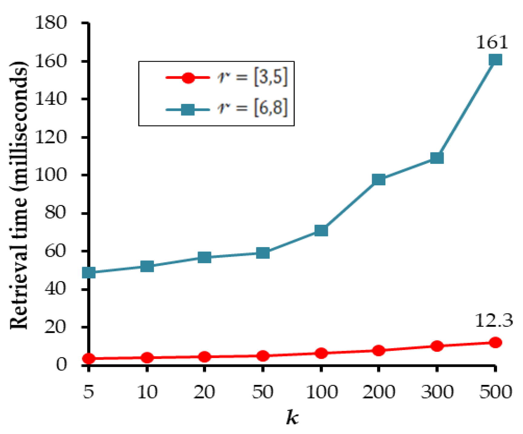
Furthermore, to evaluate the effect of $𝓇$ on the lattice-tree, some comparative results with different $𝓇$, i.e., [3,5] or [6,8], are shown in Figure 6. When $𝓇=\left[3,5\right]$, concept lattice structure will be embedded into the tree nodes of level 3 to 5. Likewise, when $𝓇=\left[6,8\right]$, the concept lattice structure will be embedded into the tree nodes of level 6 to 8. Figure 6 shows the retrieval time of ${\mathbb{T}}_{yelp}$ with the different $𝓇$. $k$ is the result number of TkSCQ. Obviously, when $𝓇=\left[3,5\right]$, the performance of ${\mathbb{T}}_{yelp}$ is significantly better than that of $𝓇=\left[6,8\right]$. Therefore, this paper set $𝓇=\left[3,5\right]$ to initialize the lattice-tree index structure, i.e., ${\mathbb{T}}_{yelp}$ and ${\mathbb{T}}_{amap}$.

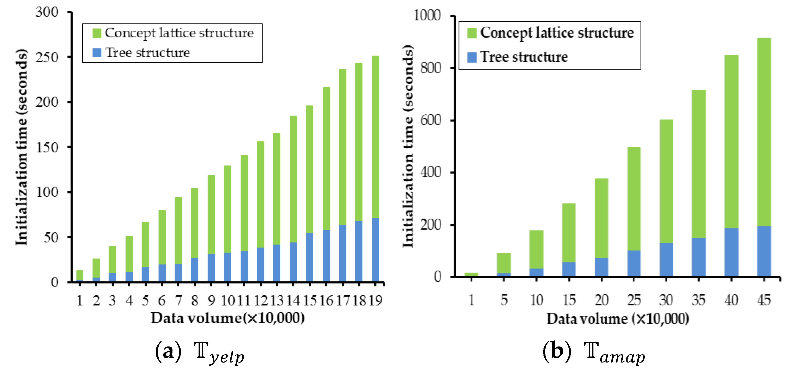
Based on the above settings of $\delta$ and $𝓇$, the effect of data volume to initialization time is shown in Figure 7. It is clear that the initialization time of the concept lattice structures is longer than the tree structure, and the initialization time of the lattice-tree increases linearly with the data volume. Finally, the ${\mathbb{T}}_{yelp}$’s initialization time of all data ${\mathbb{D}}_{yelp}$ is 249 s, its tree structure is 74 s and its concept lattice structures are 175 s. Likewise, ${\mathbb{T}}_{amap}$’s initialization time is 931 s, its tree structure is 180 s and its concept lattice structures are 751 s.

4.3. Evaluation and Comparison

For evaluating the performance of the lattice-tree, two baseline approaches, named Inverted-tree and Fpindex-tree that are modified from existing methods are employed to conduct the comparison. Specifically, inverted-tree is a variant of IRtree [1,2], which replaces the concept lattice structure of the tree-lattice nodes in the lattice-tree to inverted file structure, and similarly, Fpindex-tree replaces the concept lattice structure to the Fptree [25] structure. To achieve comparable results, the two approaches and the lattice-tree have the same initialization parameters, i.e., $\delta =\left[2,4\right]$ and $𝓇=\left[3,5\right]$. In the same way, their retrieval algorithms are also modified from Algorithm 2 and replace the retrieval codes of the concept lattice to the retrieval codes of the IR-tree and Fp-tree. See [1,2] and [25] for details of the inverted file and Fptree, which will not be repeated.

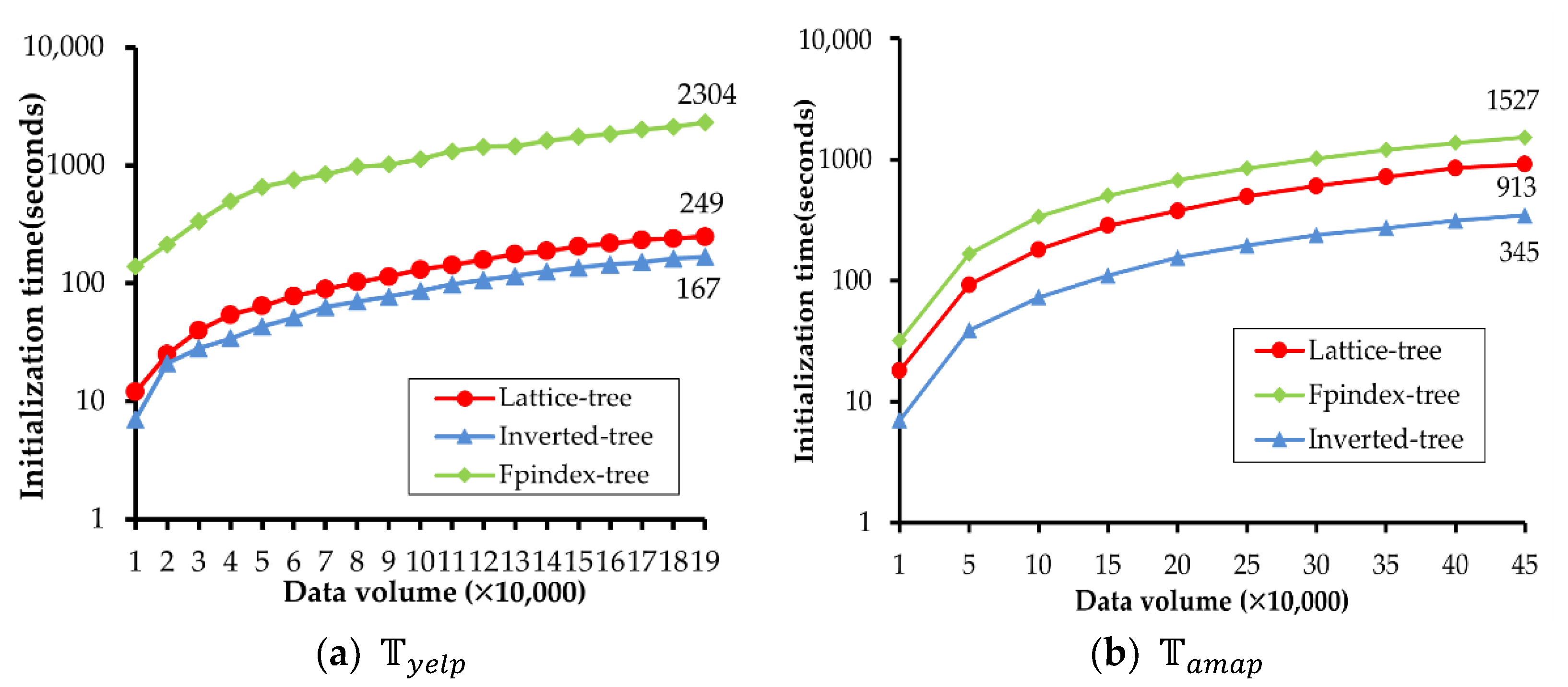
First, their initialization time cost and storage overhead are as follows. Figure 8 shows the effect of data volume on the initialization time of ${\mathbb{T}}_{yelp}$ and ${\mathbb{T}}_{amap}$. It is clear that the inverted-tree is always the best, the lattice-tree lags behind the inverted-tree, and the Fpindex-tree takes too long. Due to the inverted-tree only indexing each attribute in an inverted file, it has the shortest initialization time of 167 s in ${\mathbb{D}}_{yelp}$ and 345 s in ${\mathbb{D}}_{amap}$. The lattice-tree initialization cost time is 249 s in ${\mathbb{D}}_{yelp}$ and 913 s in ${\mathbb{D}}_{amap}$ because it takes a bit longer time to index the many-to-many relationships by the concept lattice, while the Fpindex-tree spends the longest time cost at 2304 s in ${\mathbb{D}}_{yelp}$ and 1527 s in ${\mathbb{D}}_{amap}$ to index the relationships of all existing textual attribute combinations by Fptree. Although the volume of ${\mathbb{D}}_{amap}$ is about 2.5 times that of ${\mathbb{D}}_{yelp}$, the initialization time of ${\mathbb{T}}_{amap}$ is only 0.7 times that of ${\mathbb{T}}_{yelp}$. It is clear that the initialization time of the lattice-tree is more sensitive to the keyword complexity of STBD.

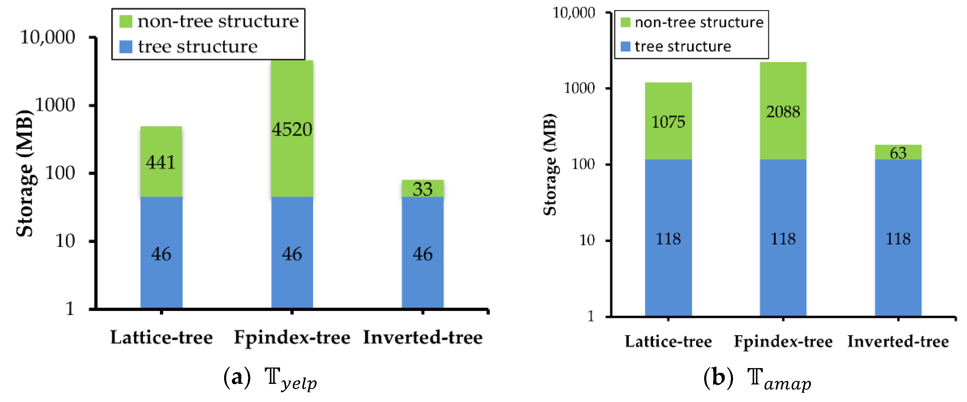
Figure 9 shows the storage overhead of three approaches. Because of their indexing mechanism, for both ${\mathbb{T}}_{yelp}$ and ${\mathbb{T}}_{amap}$, the performance ranking and differences between them are similar to those in Figure 8. In addition, these tree index structures have the same storage of 46 MB in ${\mathbb{T}}_{yelp}$ and 118 MB in ${\mathbb{T}}_{amap}$ overhead with the same parameter $\delta$, and the differences are in the non-tree structure. In other words, in ${\mathbb{T}}_{yelp}$ the concept lattice of the lattice-tree is 441 MB, the inverted file of the inverted-tree is 33 MB, and the Fptree of the Fpindex-tree is 4520 MB. In ${\mathbb{T}}_{amap}$, the concept lattice is 1075 MB, the inverted file is 63 MB, and the Fptree is 2088 MB. In addition, the differences of the lattice-tree and the inverted-tree between ${\mathbb{T}}_{yelp}$ and ${\mathbb{T}}_{amap}$ are consistent with the difference of data volume between ${\mathbb{D}}_{yelp}$ and ${\mathbb{D}}_{amap}$. However, Fpindex-tree is different from the other two. The storage overhead of its non-tree structure is more complex in ${\mathbb{D}}_{yelp}$ than ${\mathbb{D}}_{amap}$. It indicates that Fpindex-tree is more sensitive to data complexity.

Next, the performance of TkSCQ is observed in three aspects of data volume, the number of query results k, and the number of textual keywords of target objects $\widehat{d}$. Note that, to show the unbiased effectiveness, the query location and the textual features are all random, and all query results are the average of 100 times with the same query conditions.

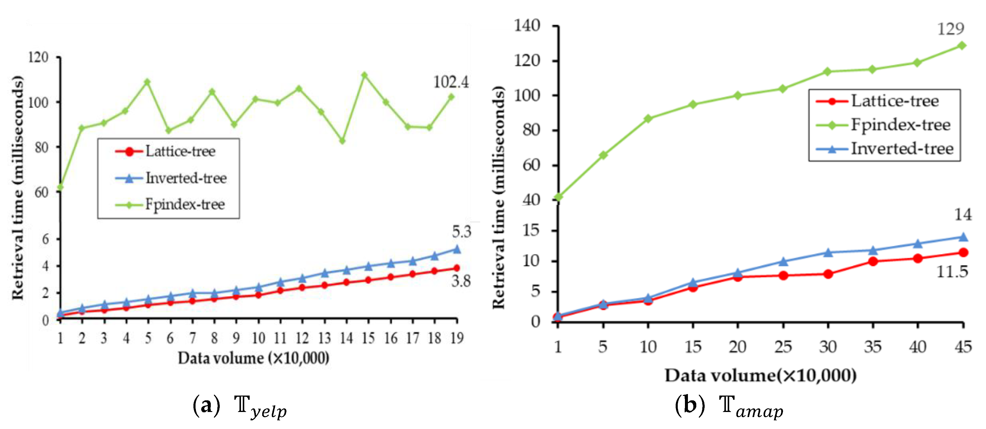
The effect of data volume on the retrieval time with $k=10$ is shown in Figure 10. It is obvious that the lattice-tree has the best performance (3.8 milliseconds in ${\mathbb{D}}_{yelp}$). The inverted-tree is at 5.3 milliseconds and the Fpindex-tree is at 102.4 milliseconds, and in ${\mathbb{D}}_{amap}$, they are 11.5 milliseconds, 14 milliseconds, and 129 milliseconds, respectively. The retrieval time of the lattice-tree increases moderately with data volume, while the inverted-tree is slightly behind the lattice-tree, and the Fpindex-tree is the worst one. These results demonstrate that with $k=10$ the retrieval performance of the lattice-tree is better than others. The retrieval time of ${\mathbb{T}}_{yelp}$ is 3.8 milliseconds (about 72% of that of the inverted-tree and 4% of the Fpindex-tree). ${\mathbb{T}}_{yelp}$ is 11.5 milliseconds (about 82% of that of Inverted-tree, and 9% of the Fpindex-tree).

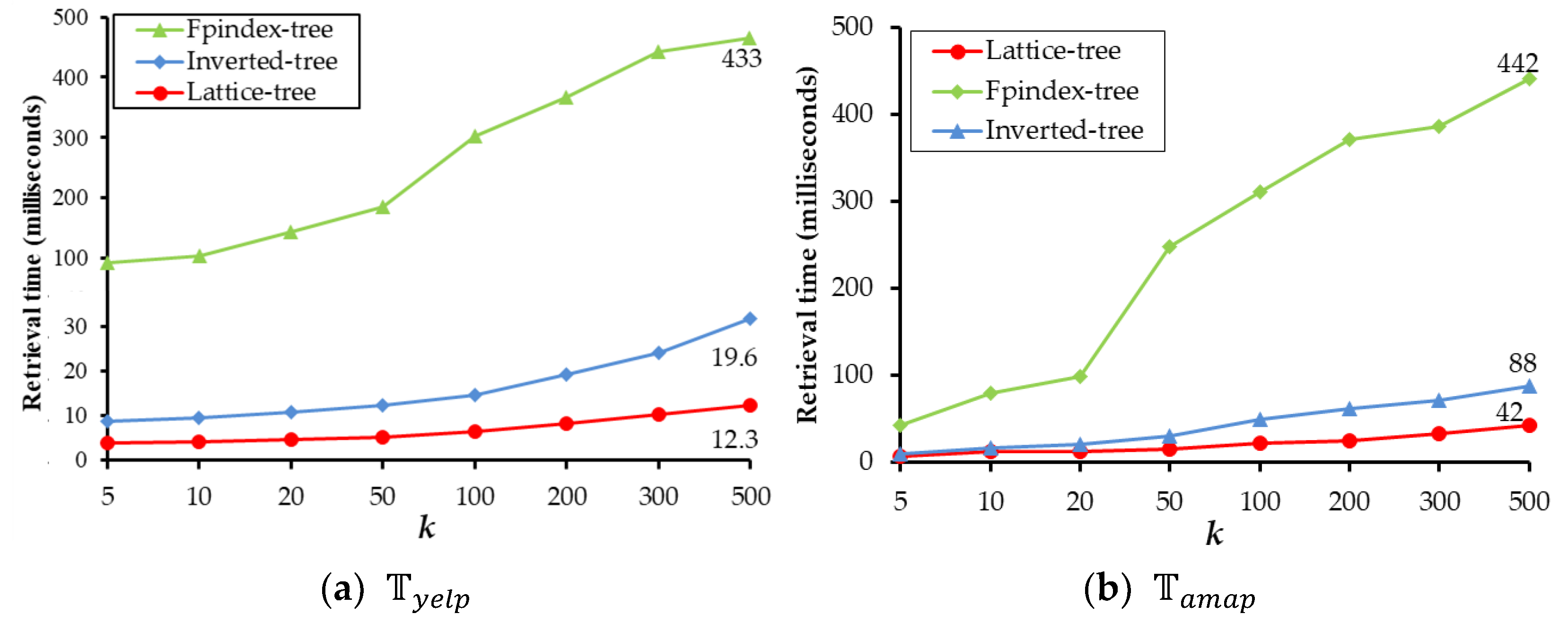
The retrieval time for $\mathbb{D}$ with different $k=\left[5, 500\right]$ is shown in Figure 11. The lattice-tree is still always the best one. Further, with the increase of k, more nodes need to be traversed to find candidates, the retrieval time of these three approaches are accelerates, and the gap between the lattice-tree and others becomes larger. When $k=500$, the retrieval time of ${\mathbb{T}}_{yelp}$, shown in Figure 11a, is 12.3 milliseconds, which is 63% of that of the inverted-tree and 3% of the Fpindex-tree. The retrieval time of ${\mathbb{T}}_{amap}$, shown in Figure 11b, is 42 milliseconds, which is 48% of that of Inverted-tree, and 10% of the Fpindex-tree.

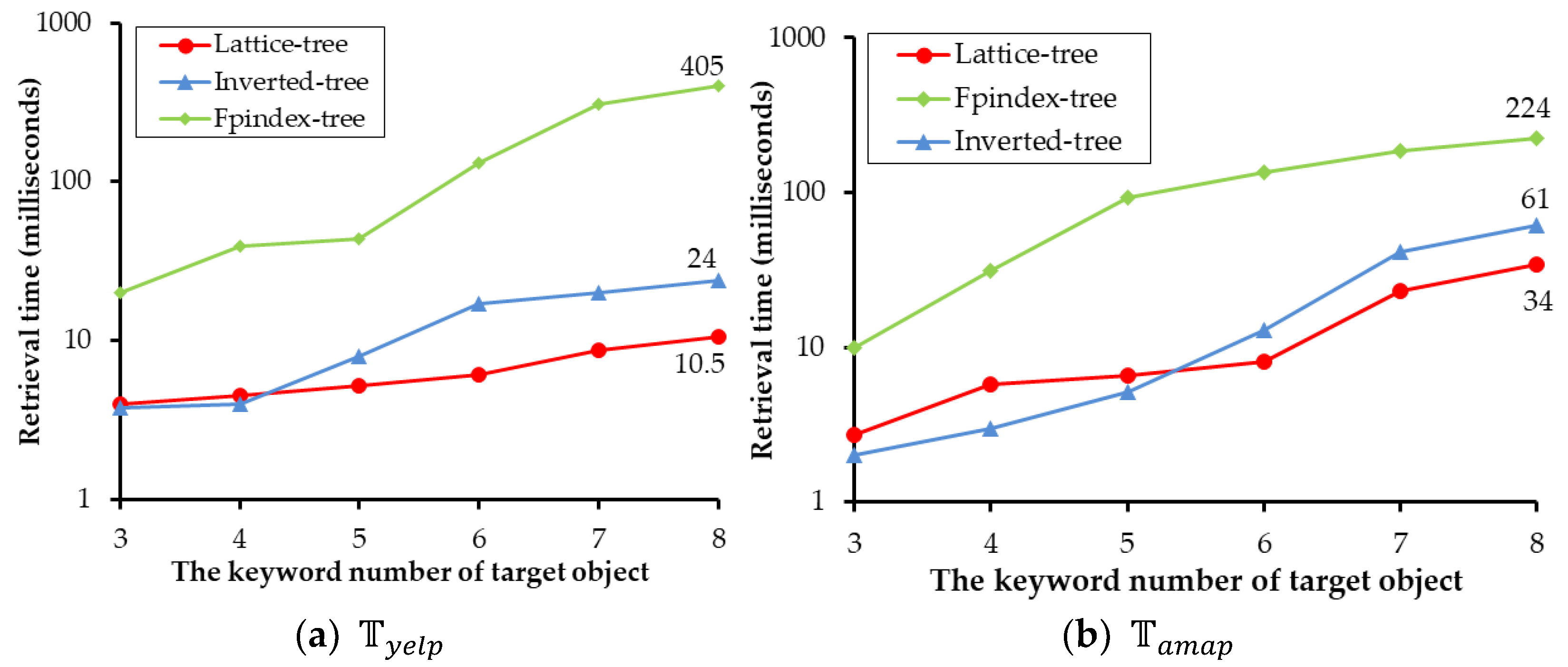
Figure 12 shows the effect of the keyword number of target object $\widehat{d}$ to retrieval time. Different from the general TkSKQ algorithm, the inputs of TkSCQ are the location point $p$, the result number $k$, and the target object $\widehat{d}$. The keyword number of $\widehat{d}$ is related to the complexity of the query because the keywords of $\widehat{d}$ need to be retrieved to match the textual features of spatial objects. In Figure 12, the indicator is in the range of 3 to 8. When its value is small (3, 4, or 5), the performance of the inverted-tree is slightly better than the lattice-tree in ${\mathbb{D}}_{yelp}$ or ${\mathbb{D}}_{amap}$. When its value is in 5 to 8, the lattice-tree is obviously better than the inverted-tree, and their gap increases with the increases of the indicator, while the Fpindex-tree is the worst one. In the complex case, when the keyword number of the target object is 8, the lattice-tree has the best performance, the retrieval time of ${\mathbb{T}}_{yelp}$ is 12 milliseconds (63% of that of the inverted-tree and 3% of the Fpindex-tree), and the retrieval time of ${\mathbb{T}}_{amap}$ is 34 milliseconds (56% of that of the inverted-tree and 15% of the Fpindex-tree).

In this section, the performance of the proposed lattice-tree is validated in comparison with two baseline index structures, the inverted-tree and the Fpindex-tree, in terms of initialization cost and TkSCQ. For ${\mathbb{D}}_{yelp}$ or ${\mathbb{D}}_{amap}$, the initialization time and storage overhead of the lattice-tree is a little worse than that of the inverted-tree, because the inverted-tree only indexes single textual features. This is much less than the Fpindex-tree that has a huge tree structure to index all features combinations of spatial objects. Regarding retrieval time, it is no doubt that the lattice-tree index structure always has the best retrieval performance with the different data volume, $k$, and the keyword number of the target object, especially in the case of the complex query conditions. The reason for this is that the concept lattice structure can organize the complex relationships between spatial objects into a concise lattice structure and supply an efficient searching way to retrieve STC by only traversing the lattice structure once. In addition, the retrieval performance of the lattice-tree is also more stable than others in ${\mathbb{T}}_{yelp}$ and ${\mathbb{T}}_{amap}$, while, with the increase in data volume and complexity, the retrieval performance of the inverted-tree and the Fpindex-tree tend to decline rapidly.

5. Conclusions

Motivated by the fact that spatial textual big data have been given more dimensionality, huge data volume and the complexity of the non-spatial textual features have both brought challenges to the retrieval of the many-to-many relationships between spatial objects and textual features. Mining rich spatial textual relationships and inferring user’s query intentions may provide a user with more satisfactory results. This paper hopes to enable the spatial textual concept STC to form many-to-many relationships and develop the specific index structure lattice-tree to maintain them. The Top-k spatial concept query (TkSCQ) algorithm is also developed to address the user’s intention and answer the similar spatial objects based on STC. A series of extensive experiments are deployed on two spatial textual big datasets to evaluate the proposed lattice-tree and TkSCQ in comparison with two baseline approaches, the inverted-tree and the Fpindex-tree. The experimental results on the lattice-tree explain the rationality of its structure and show that when the concept lattice is embedded into tree nodes of levels 3 to 5, the performance of the lattice-tree is better. The experimental results on TkSCQ also demonstrate that the proposed lattice-tree obviously has better retrieval efficiency, especially in spatial textual big data. When the number of query results is 500, the retrieval performance of the lattice-tree in ${\mathbb{D}}_{yelp}$ is about 1.6 times that of the inverted-tree and 35 times that of the Fpindex-tree, and the retrieval performance of the lattice-tree in ${\mathbb{D}}_{amap}$ is about two times that of the inverted-tree and 10 times that of the Fpindex-tree. In addition, on ${\mathbb{D}}_{yelp}$ and ${\mathbb{D}}_{amap}$ with different data volume and keyword complexity, the lattice-tree always shows a more stable retrieval performance than the other two methods.

Future work will be carried out in the following three directions. First, the scalability of the lattice-tree will be examined with larger datasets. Second, the size of the lattice-tree cannot grow unlimitedly. As such, a more flexible partitioned index may be an alternative. Third, the tree structure of the lattice-tree may be optimized to explore the possibility of further improving its performance.

References

- Cong, G.; Jensen, C.S.; Wu, D. Efficient retrieval of the top-k most relevant spatial web objects. Proc. VLDB Endow. 2009, 2, 337–348. [Google Scholar] [CrossRef] [Green Version]
- Li, Z.; Lee, K.C.K.; Zheng, B.; Lee, W.C.; Lee, D.L.; Wang, X. IR-Tree: An Efficient Index for Geographic Document Search. IEEE Trans. Knowl. Data Eng. 2011, 23, 585–599. [Google Scholar] [CrossRef]
- Zhang, C.; Zhang, Y.; Zhang, W.; Lin, X. Inverted Linear Quadtree: Efficient Top k Spatial Keyword Search. IEEE Trans. Knowl. Data Eng. 2016, 28, 1706–1721. [Google Scholar] [CrossRef]
- Hong, H.J.; Chiu, G.M.; Tsai, W.Y. A single quadtree-based algorithm for top-k spatial keyword query. Pervasive Mob. Comput. 2017, 42, 93–107. [Google Scholar] [CrossRef]
- Vaid, S.; Jones, C.B.; Joho, H.; Sanderson, M. Spatio-textual indexing for geographical search on the web. Int. Symp. Spat. Temporal Databases 2005, 3633, 218–235. [Google Scholar]
- Luo, S.; Luo, Y.; Zhou, S.; Cong, G.; Guan, J. DISKs: A system for distributed spatial group keyword search on road networks. Proc. VLDB Endow. 2012, 5, 1966–1969. [Google Scholar] [CrossRef]
- Gao, Y.; Zhao, J.; Zheng, B.; Chen, G. Efficient Collective Spatial Keyword Query Processing on Road Networks. IEEE Trans. Intell. Transp. Syst. 2016, 17, 469–480. [Google Scholar] [CrossRef]
- Su, S.; Zhao, S.; Cheng, X.; Bi, R.; Cao, X.; Wang, J. Group-based collective keyword querying in road networks. Inf. Processing Lett. 2017, 118, 83–90. [Google Scholar] [CrossRef] [Green Version]
- Regalado, A.; Goncalves, M.; Abad-Mota, S. Evaluating Skyline Queries on Spatial Web Objects. Database Expert Syst. Appl. 2012, 7447, 416–423. [Google Scholar]
- Li, J.; Wang, H.; Li, J.; Gao, H. Skyline for geo-textual data. GeoInformatica 2016, 20, 453–469. [Google Scholar] [CrossRef]
- Shi, J.; Wu, D.; Mamoulis, N. Textually relevant spatial skylines. IEEE Trans. Knowl. Data Eng. 2016, 28, 224–237. [Google Scholar] [CrossRef] [Green Version]
- Chen, G.; Zhao, J.; Gao, Y.; Chen, L.; Chen, R. Time-Aware Boolean Spatial Keyword Queries. IEEE Trans. Knowl. Data Eng. 2017, 29, 2601–2614. [Google Scholar] [CrossRef]
- Mehta, P.; Skoutas, D.; Voisard, A. Spatio-temporal keyword queries for moving objects. In Proceedings of the 23rd SIGSPATIAL International Conference on Advances in Geographic Information Systems. Association for Computing Machinery, New York, NY, USA, 1–4 November 2015; Volume 55. [Google Scholar]
- Nepomnyachiy, S.; Gelley, B.; Jiang, W.; Minkus, T. What, where, and when: Keyword search with spatio-temporal ranges. In Proceedings of the 8th Workshop on Geographic Information Retrieval, Dallas, TX, USA, 1–8 November 2014; Association for Computing Machinery: New York, NY, USA, 2014; Volume 2. [Google Scholar]
- Zhang, D.; Tan, K.L.; Tung, A.K.H. Scalable top-k spatial keyword search. In Proceedings of the 16th International Conference on Extending Database Technology, Genoa, Italy, 18–22 March 2013; Association for Computing Machinery: New York, NY, USA, 2013; pp. 359–370. [Google Scholar]
- Christoforaki, M.; He, J.; Dimopoulos, C.; Markowetz, A.; Suel, T. Text vs. space: Efficient geo-search query processing. In Proceedings of the 20th ACM International Conference on Information and Knowledge Management, Glasgow, UK, 24–28 October 2011; Association for Computing Machinery: New York, NY, USA, 2011; pp. 423–432. [Google Scholar]
- Felipe, I.D.; Hristidis, V.; Rishe, N. Keyword Search on Spatial Databases. In Proceedings of the 2008 IEEE 24th International Conference on Data Engineering, Cancun, Mexico, 7–12 April 2008; pp. 656–665. [Google Scholar]
- Zhang, D.; Chee, Y.M.; Mondal, A.; Tung, A.K.H.; Kitsuregawa, M. Keyword Search in Spatial Databases: Towards Searching by Document. In Proceedings of the 2009 IEEE 25th International Conference on Data Engineering, Shanghai, China, 29 March–2 April 2009; pp. 688–699. [Google Scholar]
- Wu, D.; Yiu, M.L.; Cong, G.; Jensen, C.S. Joint Top-K Spatial Keyword Query Processing. IEEE Trans. Knowl. Data Eng. 2012, 24, 1889–1903. [Google Scholar] [CrossRef] [Green Version]
- Xu, J.; Sun, J.; Zhou, R.; Liu, C.; Yin, L. CISK: An interactive framework for conceptual inference based spatial keyword query. Neurocomputing 2021, 428, 368–375. [Google Scholar] [CrossRef]
- Wille, R. Restructuring lattice theory: An approach based on hierarchies of concepts. In NATO Advanced Study Institutes Series; Rival, I., Ed.; Series C—Mathematical and Physical Sciences; Springer: Dordrecht, The Netherlands, 1982; Volume 83, pp. 445–470. [Google Scholar]
- Kainz, W.; Egenhofer, M.J.; Greasley, I. Modelling spatial relations and operations with partially ordered sets. Int. J. Geogr. Inf. Syst. 1993, 7, 215–229. [Google Scholar] [CrossRef]
- Bian, F.; Li, J.; Zhang, W.; Hu, R.; Wang, J.; Li, L.; Wu, W.; Liu, W.; Wang, H.; Zhang, H.; et al. A Research about Spatial Association Rule Mining Based on Concept Lattice. In Proceedings of the 2007 International Conference on Wireless Communications, Networking and Mobile Computing, Shanghai, China, 21–25 September 2007; pp. 5979–5982. [Google Scholar]
- Tripathy, A.; Mishra, L.; Patra, P.K. A multi dimensional design framework for querying spatial data using concept lattice. In Proceedings of the 2010 IEEE 2nd International Advance Computing Conference, Patiala, India, 19–20 February 2010; pp. 394–399. [Google Scholar]
- Han, J.; Pei, J.; Yin, Y. Mining Frequent Patterns without Candidate Generation. ACM SIGMOD Record 2000, 29, 1–12. [Google Scholar] [CrossRef]
- Cao, X.; Cong, G.; Jensen, C.S. Retrieving top-k prestige-based relevant spatial web objects. Proc. VLDB Endow. 2010, 3, 373–384. [Google Scholar] [CrossRef]
- Zhang, P.; Lin, H.; Yao, B.; Lu, D. Level-aware collective spatial keyword queries. Inf. Sci. 2017, 378, 194–214. [Google Scholar] [CrossRef]
- Fang, Y.; Cheng, R.; Cong, G.; Mamoulis, N.; Li, Y. On Spatial Pattern Matching. In Proceedings of the 2018 IEEE 34th International Conference on Data Engineering, Paris, France, 16–19 April 2018; pp. 293–304. [Google Scholar]
- Ahuja, R.; Armenatzoglou, N.; Papadias, D.; Fakas, G.J. Geo-Social Keyword Search. Adv. Spat. Temporal Databases. SSTD 2015, 9239, 431–450. [Google Scholar]
- Jiang, J.; Lu, H.; Yang, B.; Cui, B. Finding top-k local users in geo-tagged social media data. In Proceedings of the 2015 IEEE 31st International Conference on Data Engineering, Seoul, Korea, 13–17 April 2015; pp. 267–278. [Google Scholar]
- Wu, D.; Li, Y.; Choi, B.; Xu, J. Social-Aware Top-k Spatial Keyword Search. In Proceedings of the 2014 IEEE 15th International Conference on Mobile Data Management, Brisbane, QLD, Australia, 14–18 July 2014; pp. 235–244. [Google Scholar]
- Shekhar, S.; Gunturi, V.; Evans, M.R.; Yang, K.S. Spatial big-data challenges intersecting mobility and cloud computing. In Proceedings of the Eleventh ACM International Workshop on Data Engineering for Wireless and Mobile Access, Scottsdale, AZ, USA, 1–6 May 2012; Association for Computing Machinery: New York, NY, USA, 2012. [Google Scholar]
- Zhao, L.; Chen, L.; Ranjan, R.; Choo, K.K.R.; He, J. Geographical information system parallelization for spatial big data processing: A review. Clust. Comput. 2016, 19, 139–152. [Google Scholar] [CrossRef]
- Göbel, R.; Henrich, A.; Niemann, R.; Blank, D. A hybrid index structure for geo-textual searches. In Proceedings of the 18th ACM Conference on Information and Knowledge Management, Hong Kong, China, 2–6 November 2009; Association for Computing Machinery: New York, NY, USA, 2009; pp. 1625–1628. [Google Scholar]
- Wu, D.; Cong, G.; Jensen, C.S. A framework for efficient spatial web object retrieval. VLDB J. 2012, 21, 797–822. [Google Scholar] [CrossRef]
- Khodaei, A.; Shahabi, C.; Li, C. Hybrid Indexing and Seamless Ranking of Spatial and Textual Features of Web Documents. Database Expert Syst. Appl. 2010, 6261, 450–466. [Google Scholar]
- Chen, Y.Y.; Suel, T.; Markowetz, A. Efficient query processing in geographic web search engines. In Proceedings of the 2006 ACM SIGMOD International Conference on Management of Data, Chicago, IL, USA, 27–29 June 2006; Association for Computing Machinery: New York, NY, USA, 2006; pp. 277–288. [Google Scholar]
- Upadhyay, P.; Pandey, M.K.; Kohli, N. Periodic pattern mining from spatio-temporal database using novel global pollination artificial fish swarm optimizer-based clustering and modified FP tree. Soft Comput. 2021, 25, 4327–4344. [Google Scholar] [CrossRef]
- Zhang, J.; Kong, X.; Philip, S.Y. Predicting Social Links for New Users across Aligned Heterogeneous Social Networks. In Proceedings of the 2013 IEEE 13th International Conference on Data Mining, Dallas, TX, USA, 7–10 December 2013; pp. 1289–1294. [Google Scholar]
- Hristova, D.; Noulas, A.; Brown, C.; Musolesi, M.; Mascolo, C. A multilayer approach to multiplexity and link prediction in online geo-social networks. EPJ Data Sci. 2016, 5, 24. [Google Scholar] [CrossRef] [PubMed] [Green Version]
- Chen, X.; Xu, J.; Zhou, R.; Liu, C.; Fang, J.; Zhao, L. S2R-tree: A pivot-based indexing structure for semantic-aware spatial keyword search. Geoinformatica 2020, 24, 3–25. [Google Scholar] [CrossRef]
- Carpineto, C.; Romano, G. A Lattice Conceptual Clustering System and Its Application to Browsing Retrieval. Mach. Learn. 1996, 24, 95–122. [Google Scholar] [CrossRef] [Green Version]
- Nguyen, P.H.P.; Corbett, D. A basic mathematical framework for conceptual graphs. IEEE Trans. Knowl. Data Eng. 2006, 18, 261–271. [Google Scholar] [CrossRef] [Green Version]
- Tu, X.; Wang, Y.; Zhang, M.; Wu, J. Using Formal Concept Analysis to Identify Negative Correlations in Gene Expression Data. IEEE/ACM Trans. Comput. Biol. Bioinform. 2016, 13, 380–391. [Google Scholar] [CrossRef]
- Zou, C.; Zhang, D.; Wan, J.; Hassan, M.M.; Lloret, J. Using Concept Lattice for Personalized Recommendation System Design. IEEE Syst. J. 2017, 11, 305–314. [Google Scholar] [CrossRef]
- Sampath, S.; Sprenkle, S.; Gibson, E.; Pollock, L.; Greenwald, A.S. Applying Concept Analysis to User-Session-Based Testing of Web Applications. IEEE Trans. Softw. Eng. 2007, 33, 643–658. [Google Scholar] [CrossRef] [Green Version]
- Guttman, A. R-trees: A dynamic index structure for spatial searching. In Proceedings of the 1984 ACM SIGMOD International Conference on Management of Data, Boston, MA, USA, 18–21 June 1984; Association for Computing Machinery: New York, NY, USA, 1984; pp. 47–57. [Google Scholar]
Figure 1.
A simple example of SKQ.
Figure 2.
An example of concept lattice.
Figure 3.
The framework of lattice-tree.
Figure 4.
The flowchart of the TkSCQ algorithm.
Figure 5.
The initialization time of each level in .
Figure 6.
The effect of to reieval time of .
Figure 7.
The effect of data volume to initialization time.
Figure 8.
The effect of data volume on the initialization time.
Figure 9.
The storage overhead.
Figure 10.
The effect of data volume to the retrieval time with .
Figure 11.
The effect of k to the retrieval time.
Figure 12.
The effect of the keyword number of target object to retrieval time.