Effects of Pansharpening on Vegetation Indices

Abstract

This study evaluated the effects of image pansharpening on Vegetation Indices (VIs), and found that pansharpening was able to downscale single-date and multi-temporal Landsat 8 VI data without introducing significant distortions in VI values. Four fast pansharpening methods—Fast Intensity-Hue-Saturation (FIHS), Brovey Transform (BT), Additive Wavelet Transform (AWT), and Smoothing Filter-based Intensity Modulation (SFIM)—and two VIs—Normalized Difference Vegetation Index (NDVI) and Simple Ratio (SR)—were tested. The NDVI and SR formulas were both found to cause some spatial information loss in the pansharpened multispectral (MS) bands, and this spatial information loss from VI transformations was not specific to Landsat 8 imagery (it will occur for any type of imagery). BT, SFIM, and other similar pansharpening methods that inject spatial information from the panchromatic (Pan) band by multiplication, lose all of the injected spatial information after the VI calculations. FIHS, AWT, and other similar pansharpening methods that inject spatial information by addition, lose some spatial information from the Pan band after VI calculations as well. Nevertheless, for all of the single- and multi-date VI images, the FIHS and AWT pansharpened images were more similar to the higher resolution reference data than the unsharpened VI images were, indicating that pansharpening was effective in downscaling the VI data. FIHS best enhanced the spectral and spatial information of the single-date and multi-date VI images, followed by AWT, and neither significantly over- or under-estimated VI values.

1. Introduction

Vegetation Indices (VIs) derived from satellite images are a useful data source for many agricultural, environmental, and climate studies. VIs have been used extensively for remote estimation of above-ground biomass [1], leaf area index [2], fraction of photosynthetically active radiation [3], net primary productivity [4], crop yields [5], fractional green vegetation cover [6,7], and many other important vegetation parameters for agricultural, ecological, and climate models. High resolution VI data is particularly important for monitoring small agricultural fields/small vegetation patches (to reduce the number of mixed pixels along field or patch boundaries), for monitoring sub-field/sub-patch variability in vegetation (e.g., to identify areas of vegetation stress, disease, or physical damage), and for detecting fine-scale changes in vegetation over time. However, high spatial resolution satellite imagery (i.e., around 10 m or finer) is typically only available from commercial satellites (e.g., RapidEye or WorldView-2) and can be expensive for multi-temporal analysis or monitoring large areas. Moderate resolution satellite imagery (around 10 m or coarser), on the other hand, can be relatively inexpensive or even free. Landsat data is the most commonly-used free moderate resolution data worldwide, and the newest satellite in the series, Landsat 8, has a panchromatic (Pan) band with a spatial resolution of 15 m, eight visible to shortwave-infrared bands with spatial resolutions of 30 m, and two thermal-infrared bands with spatial resolutions of 100 m [8].

Pansharpening increases the spatial resolution of the multispectral (MS) image bands using the spatial information extracted from the higher resolution Pan band, at the cost of some distortion of spectral information [9]. For Landsat 8 imagery, pansharpening can increase the resolution of the 30 m MS bands to 15 m (in theory) or near 15 m (in practice). Pansharpening is mainly used for visualization purposes (i.e., to allow for finer details to be observed in the MS imagery), but it has also been found useful for image segmentation [10,11], image classification [12,13,14], and land cover change detection [15]. Since pansharpening can improve the resolution of the MS bands, it should also improve the resolution of the VI images derived from these bands. However, no studies have focused specifically on the effects of pansharpening on VI images. VIs involve further image transformations of the pansharpened image bands, which can have additional impacts on their spectral and spatial quality, so it is necessary to evaluate the effects that these further transformations have on the pansharpened imagery. In addition, because multi-temporal VI data has many important applications, e.g., for monitoring vegetation phenology [16,17] or land use/land cover change [18], it is also necessary to test the impacts of pansharpening on multi-temporal VI data. One important question to address in particular is whether it is preferable to use pansharpened or original (unsharpened) MS imagery for single-date and multi-temporal VI analysis.

Many VIs require spectral information in the near infrared (NIR) and red wavelength regions. For example, the Normalized Difference Vegetation Index (NDVI) [19] and the Simple Ratio (SR) [20], two popular VIs, are calculated using the information in a NIR and a red spectral band. For Landsat 8, Band 4 (0.64–0.67 µm) is in the red wavelength region and Band 5 (0.85–0.88 µm) is in the NIR wavelength region. The 15 m panchromatic (Pan) band (Band 8) has a wavelength of 0.50–0.68 µm, putting it within the blue, green, and red spectral regions but outside the NIR region. Some past studies have used Landsat imagery to spatially downscale 250 m resolution MODIS VI data [21,22] by taking advantage of the similar spectral ranges of the Landsat and MODIS multispectral bands, but none have attempted to downscale Landsat 8 VI data using the satellite’s high resolution Pan band.

This study evaluated the effects of some commonly-used pansharpening methods on the spectral and spatial quality of two VIs—NDVI and SR—derived from Landsat 8’s spectral bands. Four fast pansharpening methods—Fast Intensity-Hue-Saturation (FIHS) [23], Brovey Transform (BT) [24], Additive Wavelet Transform (AWT) [25], and Smoothing Filter-based Intensity Modulation (SFIM) [26]—were tested because their speed makes them well-suited to processing large volumes of Landsat data for multi-temporal analysis and/or monitoring large geographic areas. The effects of pansharpening were tested on single-date VI images and a multi-temporal VI change image. The main significance of this study is that it is the first to test the effects of pansharpening on Landsat 8 VIs and the first to test the effects of pansharpening on multi-temporal analysis of VI images.

2. Fast Pansharpening Algorithms

The FIHS pansharpening algorithm is well-known for its speed, ease of implementation, and high degree of spatial enhancement [27]. It is given by:

MS_high = MS_low + δ

(1)

where MS_high is the pansharpened MS band, MS_low is the original MS band, δ = (Pan − I), and I is an Intensity image derived from the MS bands. The I image is intended to be a simulated image of the Pan band at the spatial resolution of the MS bands. Spatial details from Pan are obtained by subtracting the lower resolution I band from the higher resolution Pan band. FIHS then directly adds these spatial details to each MS band.

BT, another fast and easy-to-implement pansharpening method, injects the spatial details from Pan by multiplication. BT is given by:

(2)

To show the main difference between FIHS and BT, BT can be rewritten in an FIHS-form as:

(3)

From this rewritten form, it is clear that the difference between BT and FIHS is that BT includes the term (MS_low / I), which normalizes the spatial details added from Pan based on the pixel values in the MS band being sharpened.

Since the I band in FIHS and BT is calculated using the MS bands, their main weakness is color distortion due to the mismatch between the spectral range of the Pan band and the lower resolution MS bands used to calculate I [23]. If this spectral mismatching artificially increases the difference between Pan and I, too much information from Pan will be unnecessarily injected into the MS bands, and if it artificially decreases the difference between Pan and I, not enough details from Pan will be injected into the MS bands. A common approach to minimize the spectral mismatch between Pan and I is to adjust the weights of the MS bands used to derive I.Although in the conventional FIHS algorithm all MS bands that overlap with the spectral range of the Pan band are assumed to have equal weights for calculation of I, past studies have shown that adjusting band weights according to the spectral response of the sensors [28], through trial and error [23], or by multivariate regression [29] can reduce color distortion without any significant loss of spatial information. The disadvantage of image-specific band weighting techniques like multivariate regression is that they require additional pre-processing to be performed for each image, which may significantly increase processing times if many images need to be analyzed.

Aside from FIHS-like pansharpening methods, a large number of other pansharpening algorithms exist. For a recent review of the most common pansharpening methods, readers are referred to the open-access article by Amro et al. [9]. In general, many successful algorithms incorporate multiresolution information by degrading the Pan band and (sometimes) the MS bands to lower resolutions. AWT is one popular multiresolution method with similar speed to FIHS and BT. AWT is implemented by first degrading the Pan image to the resolution of the MS bands using the B₃ cubic spline filter given in Nuñez et al. [25], and then deriving the pansharpened image using the following equation, provided in an FIHS-like form by Tu et al. [27] as:

MS_high = MS_low + δ'

(4)

where δ' = (Pan − Pan_low), and Pan_low is the degraded Pan band. As seen in the formula, AWT is computationally-similar to FIHS, but the Pan_low image replaces the I image used in FIHS. AWT typically produces images with higher spectral quality than FIHS and BT because it avoids the color distortion introduced by the I image, but lower spatial quality because, in practice, the degraded Pan image does not perfectly match the spatial resolution of the MS bands [27].

Another fast multi-resolution pansharpening method is SFIM. SFIM uses a mean filter to degrade the Pan band, and it is similar to BT in that it injects spatial information into the MS bands by multiplication. SFIM is given by

(5)

where Pan'_low is the mean-filtered Pan band. SFIM is similar to the “smart” mode of the Hyperspherical Color Sharpening (HCS) algorithm proposed by Padwick et al. [30] and recently implemented in the ERDAS Imagine software package, while BT is similar to the “naïve” mode of HCS [31]. Although many studies have evaluated the effects of FIHS, BT, AWT, and SFIM on the MS bands (e.g., [10,25,27,31]), the effects of VI transformations on the pansharpened bands has not been investigated in detail. This type of investigation is necessary because VIs will have an impact on the spectral and spatial quality of the pansharpened image bands.

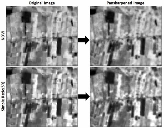
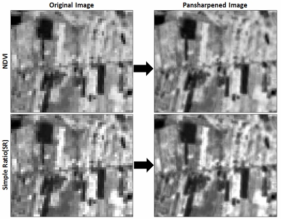
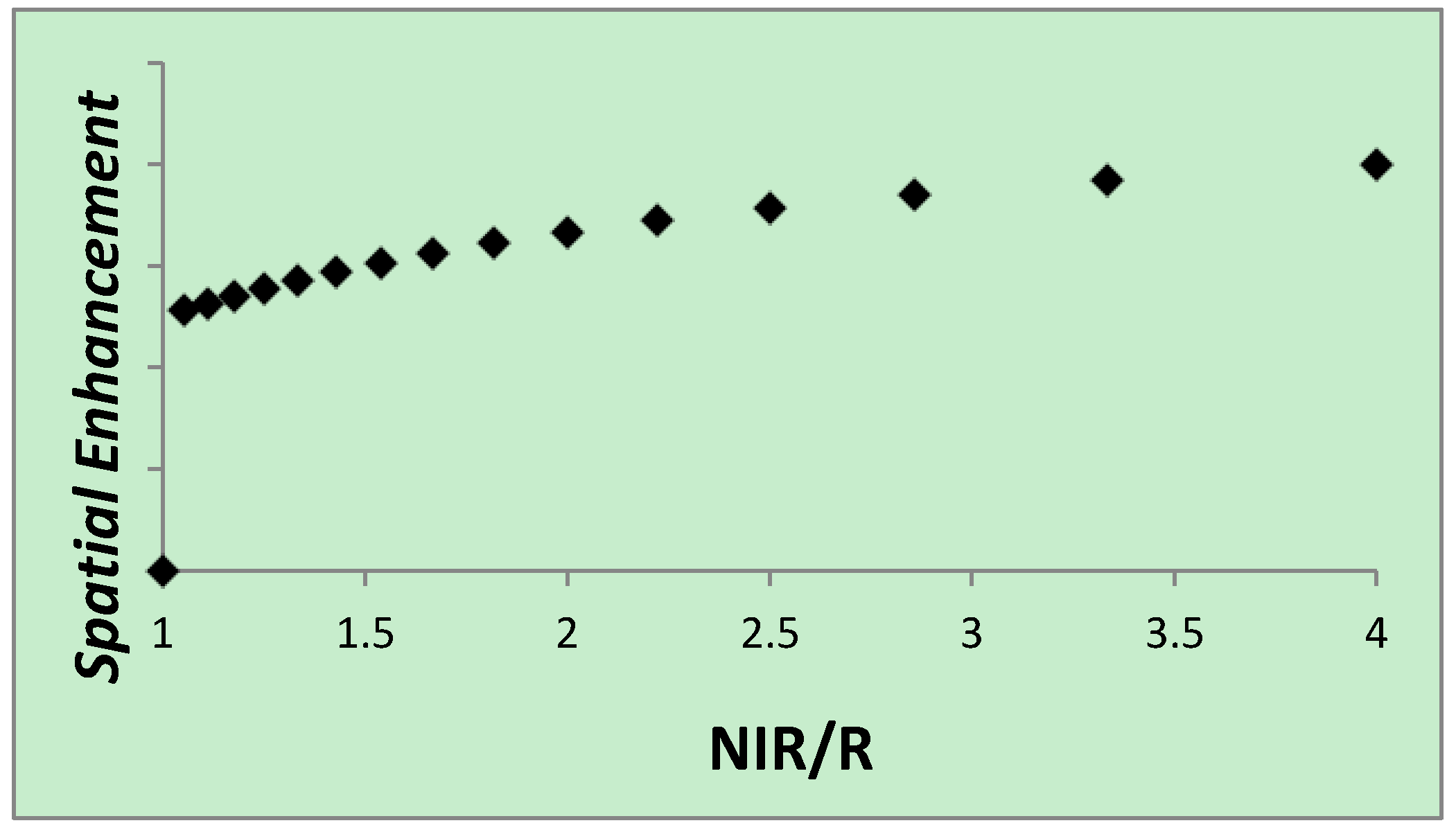
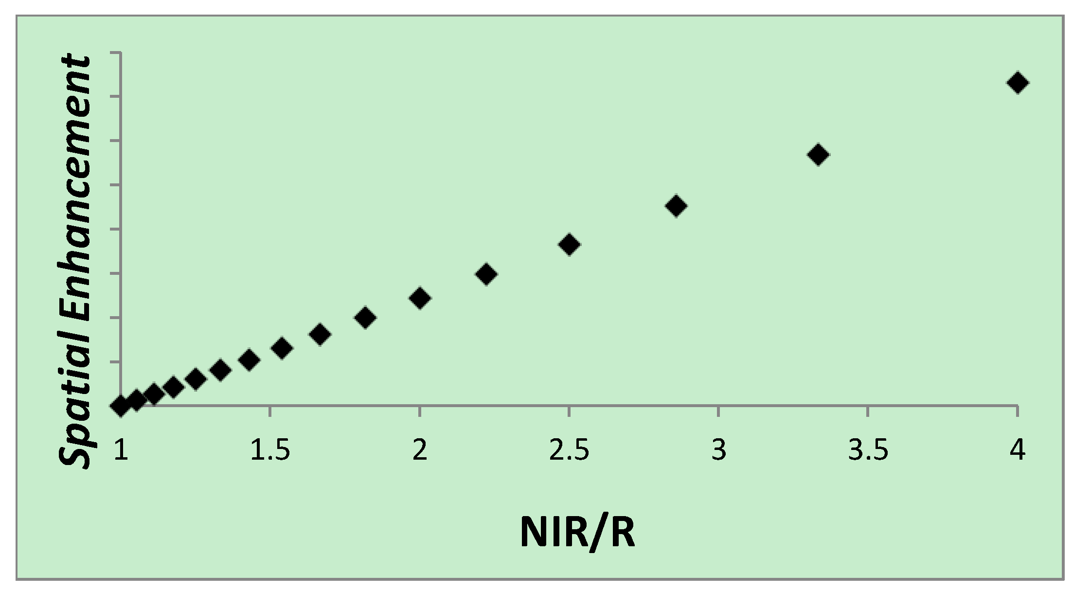
3. Effects of Pansharpening on Spatial Enhancement of Pansharpened Images

NDVI is the most commonly-used VI in remote sensing. However, as explained here, the NDVI formula reduces the spatial enhancement introduced by many pansharpening methods. To illustrate this point, a first example is given for pansharpening methods that inject spatial information by multiplication, such as BT and SFIM. As shown in Equation (6), the spatial enhancement of BT (and thus other pansharpening methods that inject spatial information by multiplication) is completely canceled out by the NDVI equation. The combined equation to derive the BT pansharpened NDVI image (NDVI_BT_high) is given by:

(6)

where NIR_low is the unsharpened NIR band, and R_low is the unsharpened red band. In the equation, the (Pan/I) terms used for BT pansharpening all cancel out, resulting in the same NDVI image as the unsharpened image bands. This was also confirmed in practice, as NDVI images generated from BT and SFIM pansharpened bands matched the NDVI images generated from the unsharpened MS bands. For pansharpening methods that inject spatial information by addition, such as FIHS and AWT, the spatial quality of the pansharpened bands is also reduced by NDVI. As an example, the combined equation to derive the FIHS pansharpened NDVI image (NDVI_FIHS_high) is given by:

(7)

In this case, the degree of spatial enhancement (i.e., the relative change in NDVI after pansharpening) varies based on the difference between NIR_low and R_low. When NIR_low = R_low there is no spatial enhancement from pansharpening, and as the difference between NIR_low and R_low increases so too does the degree of spatial enhancement from δ. This means that the spatial enhancement will be higher in vegetated areas because NIR_low will be much higher than R_low. For bare soil, built-up land, and other land cover in which NIR_low and R_low have similar values, the spatial enhancement will be less. Figure 1 shows how the spatial enhancement varies in a non-linear fashion based on the relative difference between NIR_low and R_low (i.e., NIR_low/R_low).

Figure 1. Scatterplot of the relative difference between NIR_low and R_low, calculated by NIR_low/R_low, and the relative change in NDVI values (i.e., the Spatial Enhancement) from pansharpening, calculated by |1 − NDVI_low / NDVI_high|. Numerical values on the Y-axis will change based on the value of δ, but the shape of the scatterplot does not change.

Figure 1. Scatterplot of the relative difference between NIR_low and R_low, calculated by NIR_low/R_low, and the relative change in NDVI values (i.e., the Spatial Enhancement) from pansharpening, calculated by |1 − NDVI_low / NDVI_high|. Numerical values on the Y-axis will change based on the value of δ, but the shape of the scatterplot does not change.

SR, on the other hand, is a non-normalized ratio transformation, so its effect on spatial quality is somewhat different from that of NDVI and other normalized transformations. For BT, SFIM, and other methods that inject spatial information by multiplication, the spatial enhancement from pansharpening is still completely cancelled out, as proven in Equation (8). As shown in Equation (9), for FIHS, AWT, and other additive methods, both the numerator and denominator retain the pansharpened MS information, so some spatial enhancement still occurs. Since BT and SFIM had no spatial enhancement after NDVI and SR calculations, the remainder of this study focuses only on FIHS and AWT.

(8)

(9)

Figure 2 shows that there is a linear relationship between the degree of spatial enhancement and the relative difference between NIR_low and R_low. This is unlike the non-linear relationship for NDVI. For NDVI, the spatial enhancement starts off higher than for SR (when NIR_low and R_low are fairly similar), but levels off as NIR_low becomes very large relative to R_low, while for SR the degree of spatial enhancement continues to increase. Thus NDVI will be more effective than SR for spatial enhancement in less vegetated areas, while SR will be more effective in enhancing the resolution of very highly-vegetated areas. By modifying δ and measuring the relative changes in NDVI and SR values, it was found that SR typically has higher spatial enhancement (i.e., larger relative change in VI values) than NDVI when the value of NIR_low is more than two to three times higher than R_low.

Figure 2. Scatterplot of the relative difference between NIR_low and R_low, calculated by NIR_low/R_low, and the relative change in Simple Ratio (SR) values (i.e., the Spatial Enhancement) from pansharpening, calculated by |1 − SR_low / SR_high|. Numerical values on the Y-axis will change based on the value of δ, but the shape of the scatterplot does not change.

Figure 2. Scatterplot of the relative difference between NIR_low and R_low, calculated by NIR_low/R_low, and the relative change in Simple Ratio (SR) values (i.e., the Spatial Enhancement) from pansharpening, calculated by |1 − SR_low / SR_high|. Numerical values on the Y-axis will change based on the value of δ, but the shape of the scatterplot does not change.

4. Methods

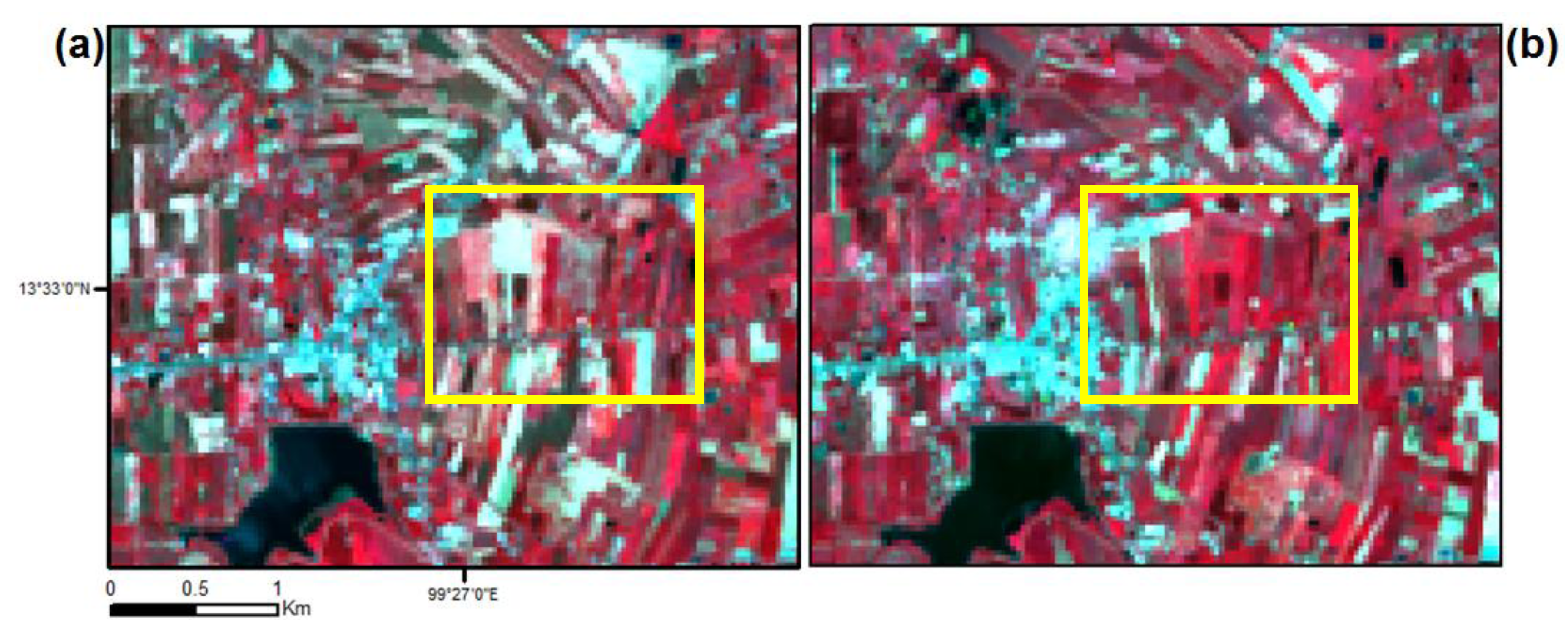
4.1. Study Area and Data

A diverse agricultural area in Tha Khoei, Thailand composed of many small fields, was chosen to analyze the impacts of pansharpening on NDVI and SR images. Two terrain corrected (Level 1T) Landsat 8 images of the study area were downloaded from the United States Geological Service EarthExplorer website [32]. The first image of the study area was acquired on 29 May 2013 and the second image was acquired on 5 November 2013. As can be seen in Figure 3, many changes vegetation occurred in the study area between the two image dates, making it a good test site for monitoring VI change. For this study, it was not important whether the changes in VI values were due to vegetation phenology, crop planting/growth/harvesting, land cover change, or other factors (e.g., atmospheric effects) because the objective was simply to determine how pansharpening effected the detection of changes in VI values. Raw digital number (DN) pixel values of the MS and Pan bands were used to avoid the introduction of any noise from atmospheric correction, but in practice, atmospheric correction is typically applied before multi-temporal analysis.

Figure 3. Color infrared Landsat 8 images acquired on 29 May 2013 (a) and 5 November 2013 (b). Red, Green, and Blue colors correspond to Band 5, Band 4, and Band 3. The yellow rectangle shows the location of the inset maps in Section 5.3.

Figure 3. Color infrared Landsat 8 images acquired on 29 May 2013 (a) and 5 November 2013 (b). Red, Green, and Blue colors correspond to Band 5, Band 4, and Band 3. The yellow rectangle shows the location of the inset maps in Section 5.3.

4.2. Image Pansharpening

For FIHS, the Landsat image Bands 2, 3, 4, and 5 were pansharpened using Equation 1. Band weights for the MS bands used to calculate I (i.e., Bands 2, 3, and 4) were determined based on the spectral responses of Landsat 8’s Pan and MS bands, obtained from [33]. The weight for the blue band (Band 2) was calculated as 0.08, the green band (Band 3) as 0.54, and the red band (Band 4) as 0.38. Using these weights, I was derived by:

I = Band 2 × 0.08 + Band 3 × 0.54 + Band 4 × 0.38

(10)

I was calculated in this way to minimize pre-processing, since the same band weights can be applied to any Landsat 8 image.

For AWT, the Landsat bands 4 and 5 were pansharpened using Equation (4). Since only these two image bands, required for the NDVI and SR calculations, need to be pansharpened with AWT (FIHS requires the other two MS bands that overlap with the Pan band to also be pansharpened), AWT is more efficient than FIHS for deriving pansharpened NDVI and SR images.

All pansharpening algorithms and VI calculations were implemented in ESRI ArcGIS 10 software using a custom ArcGIS toolbox, made available for download at [34].

4.3. Quantitative Evaluation of Pansharpened VI Images

To evaluate the spectral quality of the pansharpened VI images, prior to pansharpening the Pan band for each image date was degraded from 15 m to 30 m spatial resolution and the MS bands were degraded from 30 m to 60 m using the cubic spline filter in Section 2. Since this filtering procedure has been shown to be quite effective at simulating lower resolution images [25], it should not have a major influence on the results of the study [35]. For some examples of other suitable filters and a further discussion on the impacts of filtering on quantitative evaluations, readers are referred to [35]. The degraded 60 m MS bands were pansharpened to 30 m (using the degraded 30 m Pan band) and used to derive VI images, and these pansharpened VI images were compared with reference VI images, produced by deriving VI images from the original (un-degraded) 30 m MS bands. Four metrics were used to evaluate the quality of the pansharpened VI images: Bias [35], Correlation Coefficient (CC) [35], Mean Average Error (MAE), and Root Mean Square Error (RMSE) [35]. Since the errors in NDVI estimates were all between −1.000 and 1.000 (and many were for SR as well), the error values were multiplied by 1000 prior to computing RMSE (since squaring the errors actually reduces them for values between −1.000 and 1.000). After calculating RMSE, the values were again divided by 1000 to convert them back to meaningful VI values.

Of the metrics, Bias is sensitive only to the difference in the mean values of the reference and pansharpened images, while CC is sensitive only to the correlation between the images (and insensitive to the constant bias), and MAE and RMSE provide average per-pixel error estimates. To determine whether the pansharpened VI images or the unsharpened 60 m VI images were more similar to the reference 30 m VI images, the metrics were also calculated for the unsharpened 60 m VI images. For pansharpening to be considered as useful for downscaling VI data, the pansharpened VI images should be more similar to the reference VI images.

Multi-temporal VI quality was measured by computing Bias, CC, MAE, and RMSE for a NDVI and a SR change image. VI differencing is a simple but useful method for monitoring changes in VI values [36], so VI Difference images, derived by subtracting the VI values in the November image from the VI values in the May image, were used to evaluate the effect of pansharpening on multi-temporal VI analysis. The reference VI Difference images were derived from the original 30 m NDVI and SR images. For comparison, VI Difference images were also derived from the unsharpened 60 m VI images. By comparing the quality of the pansharpened and unsharpened VI Difference images, it is possible to determine whether or not pansharpening was effective in downscaling the multi-temporal VI data.

5. Results and Discussion

5.1. Quantitative Evaluation of Pansharpened VI Images

To ensure that the band weights used to derive the I image (for FIHS) were appropriate, the mean values of the I and Pan bands were compared as well as the correlation between δ and NDVI. The rationale for comparing the mean values is that the means of the Pan and I bands should be very similar if little global spectral distortion exists between Pan and I. In addition, since the degree of spectral mismatching between Pan and I may be different for vegetation and non-vegetation land cover if improper band weights are used [23], it is necessary to confirm that this does not occur. To test for variation in spectral mismatching, the correlation between δ and NDVI was evaluated using R². δ should not be correlated with NDVI if the mismatching between Pan and I is consistent across all NDVI values (the desirable result). For the May image, the mean value of the Pan image was 10,108 and the mean of the I image was 10,226 (a difference of 1%) and for the November image, the mean of the Pan image was 8751 and the mean of the I image was 8,849 (also a difference of 1%), indicating that there was little global spectral mismatching between Pan and I. As shown in Figure 4, in the May image the correlation between δ and NDVI, measured by R², was 0.017, and for the November image, the correlation between δ and NDVI was 0.004. Thus for both images, the spectral mismatching between Pan and I did not vary by land cover. These results indicate that the band weights used for I were appropriate for both study area images, and suggest that they may be suitable for other Landsat 8 images.

Figure 4. Scatterplots of δ and NDVI for the May (a) and November (b) Landsat images. δ = (Pan − Intensity). The low R² indicates that the degree of spectral mismatching between the Pan and Intensity images did not vary by land cover.

Figure 4. Scatterplots of δ and NDVI for the May (a) and November (b) Landsat images. δ = (Pan − Intensity). The low R² indicates that the degree of spectral mismatching between the Pan and Intensity images did not vary by land cover.

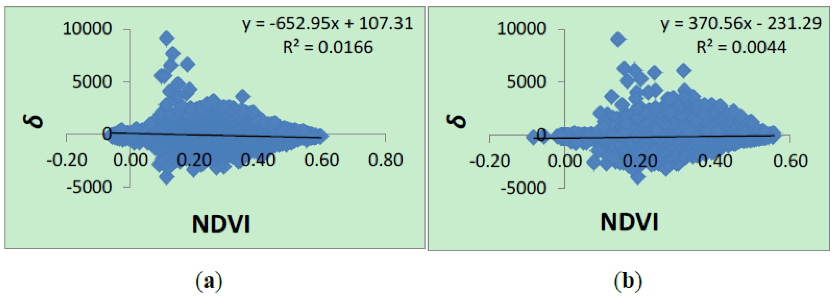
5.2. Spectral Quality of Pansharpened VI Images

Results for the single-date NDVI images, given in Table 1, indicate that neither FIHS nor AWT introduced a significant Bias in NDVI values. Thus they should not lead to any constant over- or under-estimation of vegetation parameters (e.g., above-ground biomass, leaf area index, yield, etc.). In terms of the other metrics, FIHS had the highest CC (0.963), lowest MAE (0.022), and lowest RMSE (0.031) for the May image date, followed by AWT (CC = 0.955, MAE = 0.025, RMSE = 0.034) and finally the unsharpened image (CC = 0.946, MAE = 0.027, RMSE = 0.037). For the November image, the CC, MAE, and RMSE of FIHS (0.953, 0.021, and 0.029) and AWT (0.954, 0.021, and 0.030) were similar, and slightly better than those of the unsharpened NDVI image (0.952, 0.022, and 0.030). The lesser impact of pansharpening on the November image was due to the higher spectral homogeneity of land cover on that date, which reduced the amount of spatial information injected from Pan to the MS bands. As shown in Figure 3, the May image contained a mixture of newly-planted fields interspersed with bare soil, while the November image contained mainly fully-green fields and less bare soil. The higher standard deviation of the May reference NDVI image (0.110) than the November image (0.095) also confirmed the higher homogeneity of VI values in the November image.

Table 1. Bias, Correlation Coefficient (CC), Mean Average Error (MAE), and Root Mean Square Error (RMSE) of the single-date NDVI images and the NDVI Difference image. FIHS, Fast Intensity-Hue-Saturation pansharpened imagery; AWT, Additive Wavelet Transform pansharpened imagery; 60m, unsharpened 60m resolution imagery.

NDVI Image	Spectral Information	Bias	CC	MAE	RMSE
May	FIHS	−0.004	0.963	0.022	0.031
	AWT	0.000	0.955	0.025	0.034
	60m	0.000	0.946	0.027	0.037
November	FIHS	−0.004	0.953	0.021	0.029
	AWT	−0.001	0.954	0.021	0.030
	60m	−0.001	0.952	0.022	0.030
Difference (May–Nov.)	FIHS	−0.000	0.940	0.023	0.031
	AWT	−0.001	0.935	0.025	0.033
	60m	−0.001	0.925	0.026	0.035

Table 1. Bias, Correlation Coefficient (CC), Mean Average Error (MAE), and Root Mean Square Error (RMSE) of the single-date NDVI images and the NDVI Difference image. FIHS, Fast Intensity-Hue-Saturation pansharpened imagery; AWT, Additive Wavelet Transform pansharpened imagery; 60m, unsharpened 60m resolution imagery.

NDVI Image	Spectral Information	Bias	CC	MAE	RMSE
May	FIHS	−0.004	0.963	0.022	0.031
	AWT	0.000	0.955	0.025	0.034
	60m	0.000	0.946	0.027	0.037
November	FIHS	−0.004	0.953	0.021	0.029
	AWT	−0.001	0.954	0.021	0.030
	60m	−0.001	0.952	0.022	0.030
Difference (May–Nov.)	FIHS	−0.000	0.940	0.023	0.031
	AWT	−0.001	0.935	0.025	0.033
	60m	−0.001	0.925	0.026	0.035

Results for the single-date SR images, given in Table 2, were similar to the results for the NDVI images. FIHS produced the most similar SR images to the reference SR data, followed by AWT and finally the unsharpened 60 m SR images. The improvement in the pansharpened images was again more significant in the May image than the November image due to the higher degree of heterogeneity in the May image. Figure 5 shows a map of the RMSE values for the May SR image to give an example of the spatial distribution of errors in VI values. The RMSE map of the unsharpened SR image in Figure 5d is very similar to the RMSE maps of the pansharpened SR images in Figure 5b,c, with the errors being high for linear features and other small features and low for more homogeneous areas. This similarity between the RMSE maps suggests that the errors were mainly due to the lower spatial quality of the pansharpened images than the reference image (causing VI to be underestimated in small, highly-vegetated areas and overestimated in small areas with little vegetation cover), and not due to the introduction of significant new errors in VI values from pansharpening. One region of the map in Figure 5 is highlighted to show the lower RMSE values for a narrow planted field in the pansharpened images.

Table 2. Bias, Correlation Coefficient (CC), Mean Average Error (MAE), and Root Mean Square Error (RMSE) of the single-date Simple Ratio (SR) images and the SR Difference image.

SR Image	Spectral Information	Bias	CC	MAE	RMSE
May	FIHS	0.000	0.957	0.107	0.145
	AWT	0.021	0.946	0.122	0.165
	60 m	0.023	0.936	0.132	0.178
November	FIHS	−0.007	0.943	0.105	0.138
	AWT	−0.011	0.944	0.105	0.140
	60 m	−0.011	0.941	0.108	0.144
Difference (May-Nov.)	FIHS	0.007	0.938	0.117	0.157
	AWT	0.010	0.932	0.123	0.168
	60 m	0.012	0.923	0.130	0.177

Table 2. Bias, Correlation Coefficient (CC), Mean Average Error (MAE), and Root Mean Square Error (RMSE) of the single-date Simple Ratio (SR) images and the SR Difference image.

SR Image	Spectral Information	Bias	CC	MAE	RMSE
May	FIHS	0.000	0.957	0.107	0.145
	AWT	0.021	0.946	0.122	0.165
	60 m	0.023	0.936	0.132	0.178
November	FIHS	−0.007	0.943	0.105	0.138
	AWT	−0.011	0.944	0.105	0.140
	60 m	−0.011	0.941	0.108	0.144
Difference (May-Nov.)	FIHS	0.007	0.938	0.117	0.157
	AWT	0.010	0.932	0.123	0.168
	60 m	0.012	0.923	0.130	0.177

Results for the NDVI Difference and SR Difference images are also given in Table 1 and Table 2, respectively. The results for the VI Difference images were consistent with the results for the single-date images. Namely, for both the NDVI and SR Difference images, FIHS produced the most similar results to the reference data set (i.e., lowest Bias, MAE, RMSE, and highest CC), indicating that it was the most useful pansharpening method for deriving the higher resolution multi-temporal VI images. AWT also produced more similar VI Difference images to the reference data than the unsharpened 60 m images, indicating that pansharpening can be useful for downscaling multi-temporal VI data.

Figure 5. May SR image (a), and RMSE maps of the FIHS (b) AWT (c) and unsharpened (d) SR images. Brighter pixels in (b–d) indicate higher RMSE values. The yellow rectangle shows a long, narrow planted field with lower RMSE values in the pansharpened image (b) (and slightly lower RMSE values in (c)) than in the unsharpened image (d).

Figure 5. May SR image (a), and RMSE maps of the FIHS (b) AWT (c) and unsharpened (d) SR images. Brighter pixels in (b–d) indicate higher RMSE values. The yellow rectangle shows a long, narrow planted field with lower RMSE values in the pansharpened image (b) (and slightly lower RMSE values in (c)) than in the unsharpened image (d).

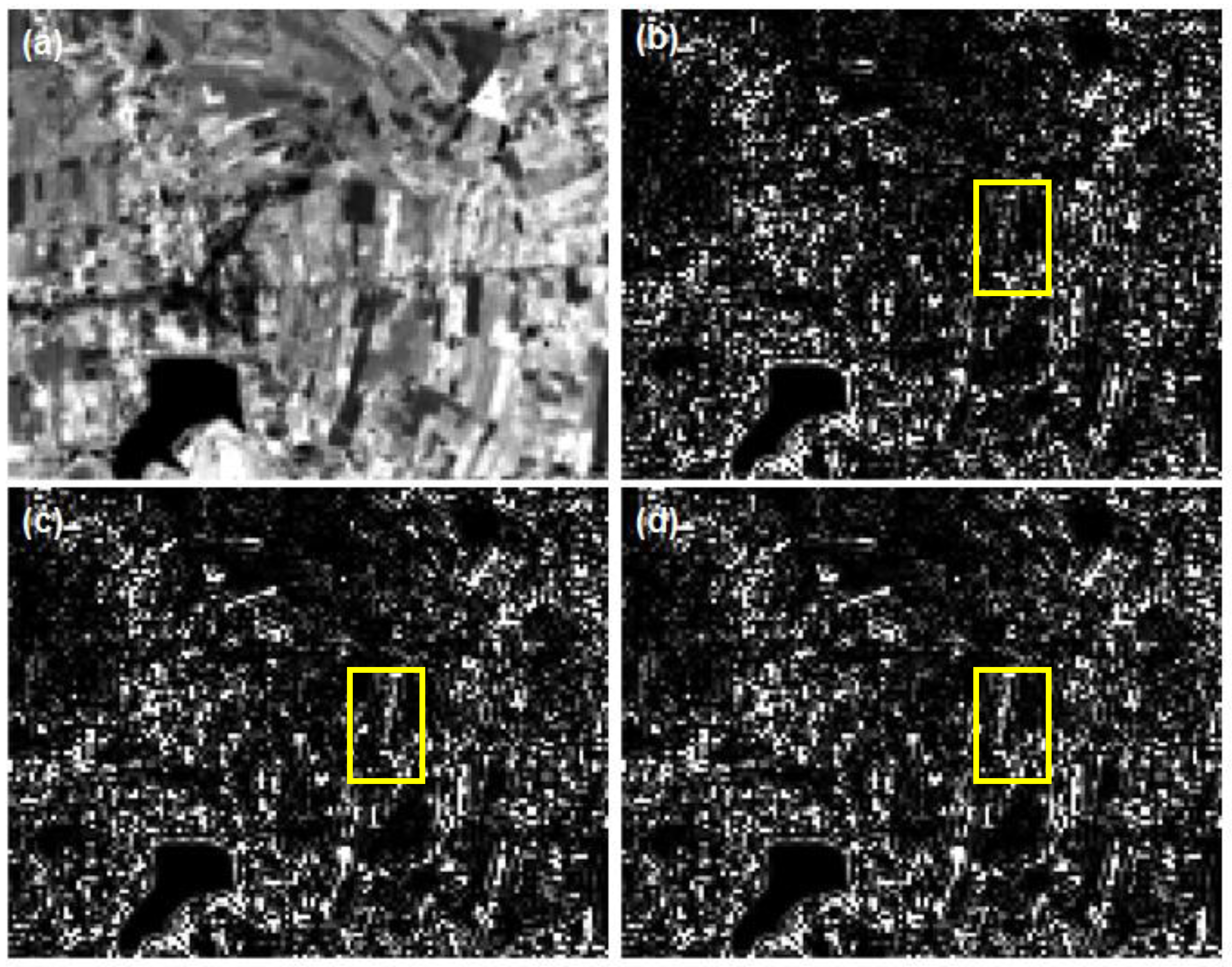
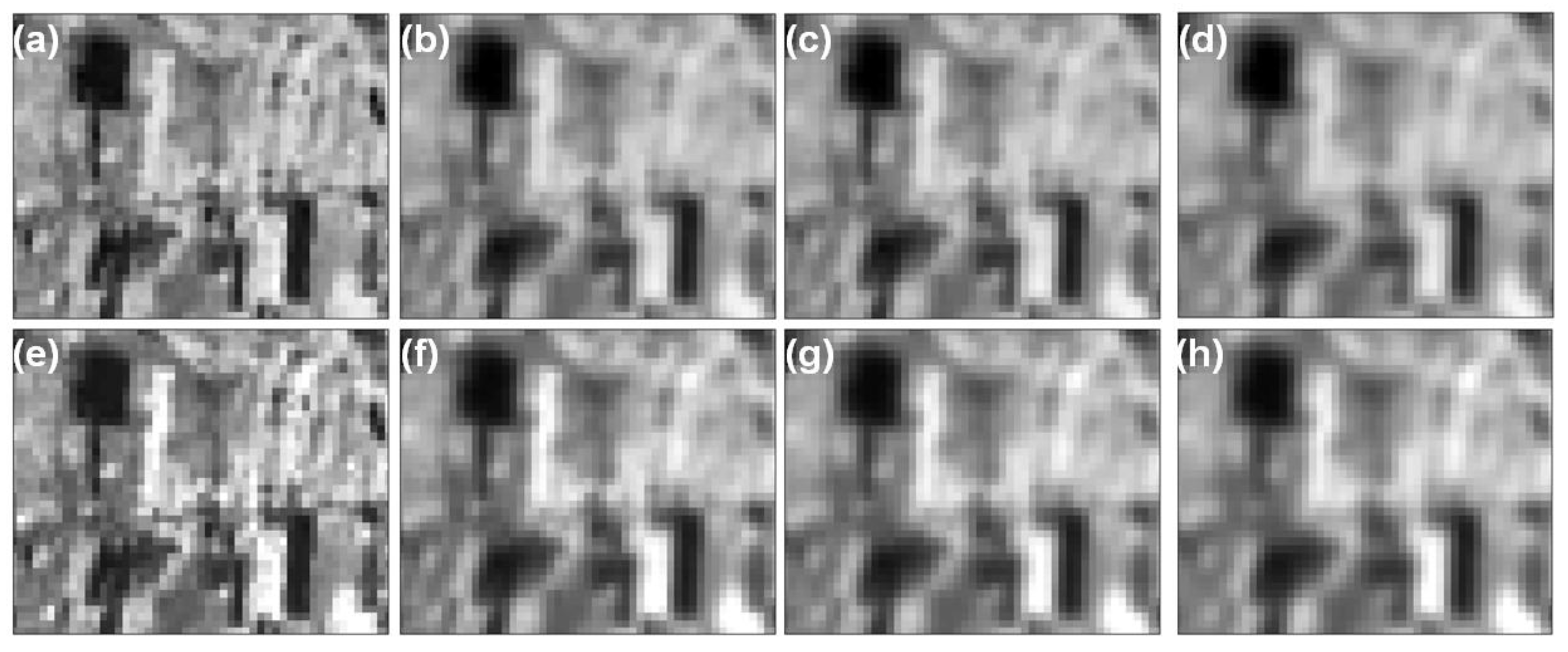
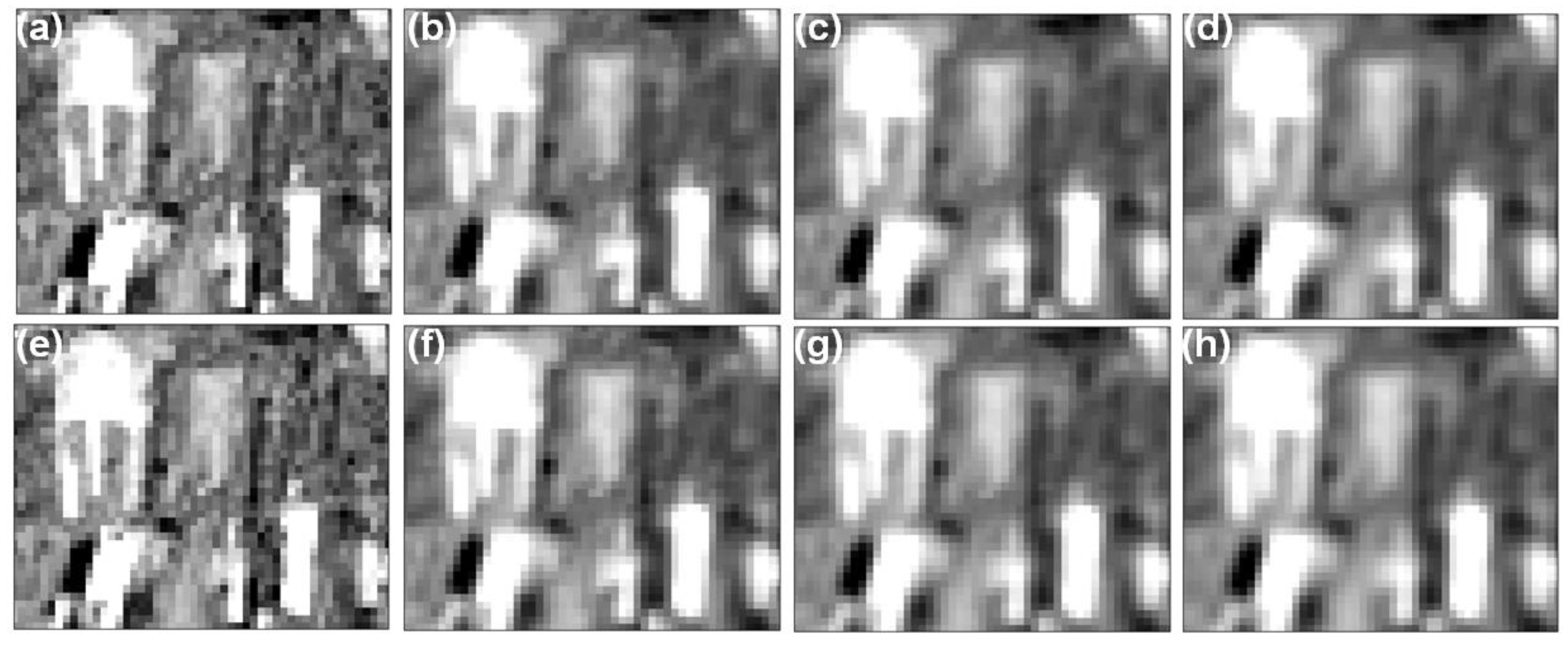
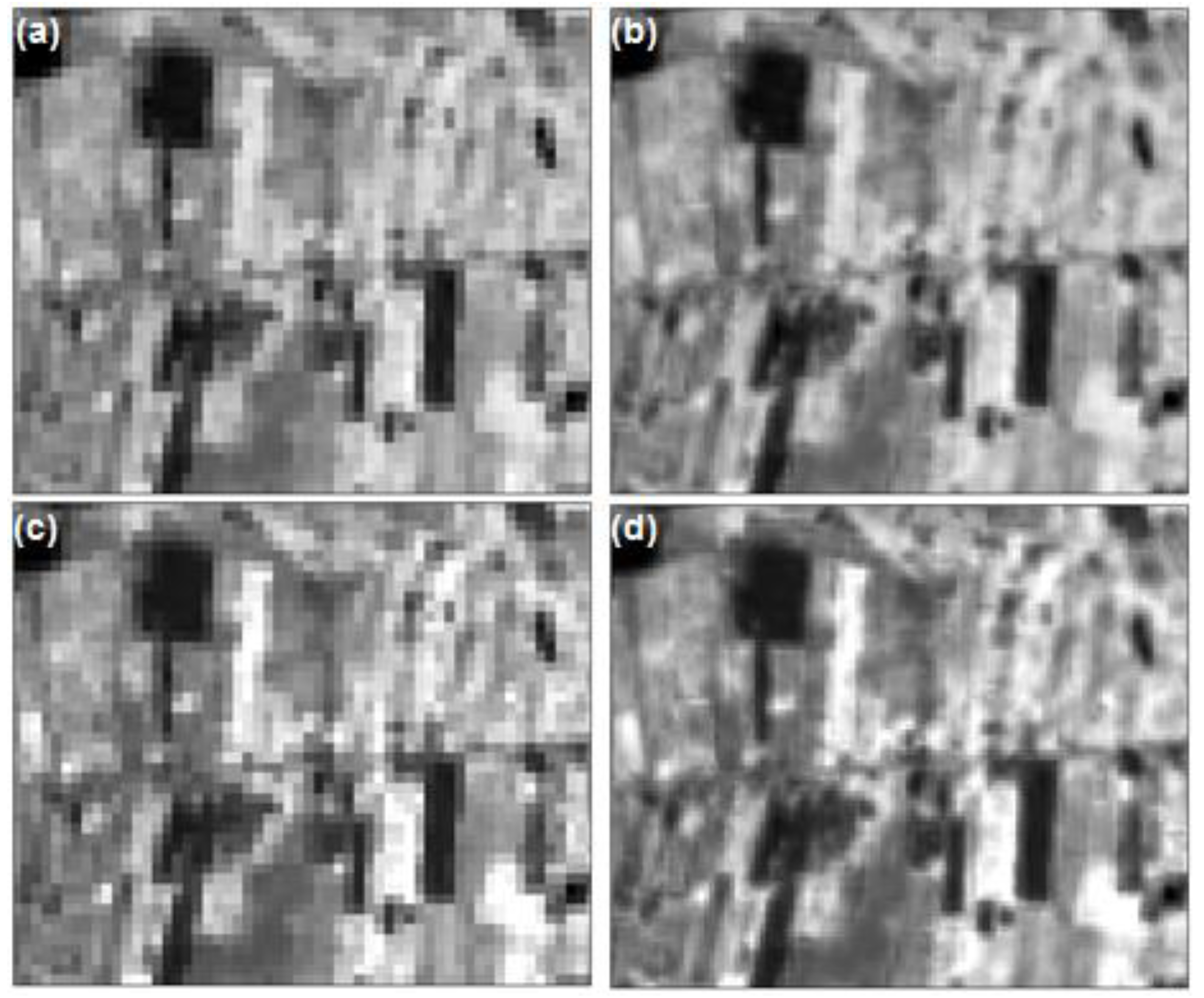
5.3. Spatial Quality of Pansharpened VI Images

To give an idea of the spatial quality of the pansharpened NDVI and SR images, Figure 6 shows subsets of the pansharpened, unsharpened, and reference images for the May image date, and Figure 7 shows subsets of the pansharpened, unsharpened, and reference VI Difference images. In Figure 6 and Figure 7, it is clear that FIHS best enhanced the spatial details of the VI images. Still, as explained in Section 3, all of the pansharpened images have lower spatial quality than the reference images because the VI equations resulted in some loss of spatial enhancement in the pansharpened bands. To give an idea of the actual spatial quality of FIHS-derived VI images at their full scale (i.e., from pansharpening the original 30 m MS bands to 15 m and then deriving the VIs), Figure 8 shows the pansharpened NDVI and SR images for the May image date.

Figure 6. Reference (a), FIHS (b), AWT (c), and unsharpened (d) NDVI images. Reference (e), FIHS (f), AWT (g), and unsharpened (h) SR images for the May image date. Brighter pixels indicate higher VI values (i.e., more green vegetation).

Figure 6. Reference (a), FIHS (b), AWT (c), and unsharpened (d) NDVI images. Reference (e), FIHS (f), AWT (g), and unsharpened (h) SR images for the May image date. Brighter pixels indicate higher VI values (i.e., more green vegetation).

Figure 7. Reference (a), FIHS (b), AWT (c), and unsharpened (d) NDVI Difference images. Reference (e), FIHS (f), AWT (g), and unsharpened (h) SR Difference images. Difference images were derived by subtracting the pixel values in the November image from those in the May image. Brighter pixels indicate an increase in VI values (i.e., increase in green vegetation) from May to November, darker pixels indicate a decrease in VI values (i.e., reduction in green vegetation).

Figure 7. Reference (a), FIHS (b), AWT (c), and unsharpened (d) NDVI Difference images. Reference (e), FIHS (f), AWT (g), and unsharpened (h) SR Difference images. Difference images were derived by subtracting the pixel values in the November image from those in the May image. Brighter pixels indicate an increase in VI values (i.e., increase in green vegetation) from May to November, darker pixels indicate a decrease in VI values (i.e., reduction in green vegetation).

Figure 8. 30 m resolution NDVI image (a) and 15 m NDVI image derived from the FIHS pansharpened bands (b). 30 m resolution SR image (c) and 15 m SR image derived from the FIHS pansharpened bands (d). Images are from the May image date. Brighter pixels indicate higher VI values (i.e., more green vegetation).

Figure 8. 30 m resolution NDVI image (a) and 15 m NDVI image derived from the FIHS pansharpened bands (b). 30 m resolution SR image (c) and 15 m SR image derived from the FIHS pansharpened bands (d). Images are from the May image date. Brighter pixels indicate higher VI values (i.e., more green vegetation).

5.4. Future Considerations for Pansharpening VI Images

Because of the loss of some spatial enhancement in the pansharpened MS bands caused by NDVI, SR, and other similar VIs, it may be necessary to rethink the way in which VI images are pansharpened if higher spatial quality is desired. For example, rather using an approach of first pansharpening the MS bands and then deriving a VI image from the pansharpened MS bands (resulting in a loss of some spatial information), it may be preferable to first derive the VI image from the unsharpened MS bands and then pansharpen this VI image. For this type of pansharpening, image fusion methods well-suited to multi-sensor image fusion (e.g., fusing optical and thermal imagery, optical and microwave imagery, etc.) such as Ehlers Fusion [37] may perform better because the pixel values in the Pan and VI images represent different types of information (visible light reflectance and vegetation abundance, respectively). Statistically- [38] or geostatistically-based [39] pansharpening methods may also be better-suited for this type of pansharpening.

6. Conclusions

This study investigated the effects of pansharpening on Vegetation Index (VI) images. Four fast pansharpening methods were tested for downscaling VI images derived from Landsat 8 data. For Brovey Transform (BT) and Smoothing Filter-based Intensity Modulation (SFIM), the two pansharpening methods that inject spatial information into the multispectral bands by multiplication, the Normalized Difference Vegetation Index (NDVI) and Simple Ratio (SR) formulas canceled out all spatial enhancement gained by pansharpening. For Fast Intensity-Hue-Saturation (FIHS) and Additive Wavelet Transform (AWT), the two pansharpening methods that inject spatial information into the multispectral bands by addition, the NDVI and SR formulas also resulted in some loss of spatial enhancement. Despite this fact, FIHS and AWT were both found to be effective in downscaling the single-date and multi-temporal VI images, as they increased their spatial resolution without introducing a significant distortion in VI values. These results indicate that it may be desirable to perform pansharpening prior to VI calculations, particularly for monitoring small agricultural fields or other small vegetation patches. Of the two pansharpening methods, FIHS was best able to downscale the VI images and VI change images. Future research is needed to: (1) identify pansharpening methods that lose less spatial information through VI calculations, and/or (2) identify alternative methods for downscaling VI images (e.g., directly fusing the unsharpened VI image with the panchromatic band).

References

1. Lu, D.; Mausel, P.; Brondı́zio, E.; Moran, E. Relationships between forest stand parameters and Landsat TM spectral responses in the Brazilian Amazon Basin. For. Ecol. Manag. 2004, 198, 149–167. [Google Scholar] [CrossRef]
2. Wang, Q.; Adiku, S.; Tenhunen, J.; Granier, A. On the relationship of NDVI with leaf area index in a deciduous forest site. Remote Sens. Environ. 2005, 94, 244–255. [Google Scholar]
3. Asner, G.P.; Wessman, C.A.; Schimel, D.S. Heterogeneity of savanna canopy structure and function from imaging spectrometry and inverse modeling. Ecol. Appl. 1998, 8, 1022–1036. [Google Scholar] [CrossRef]
4. Goward, S.N.; Tucker, C.J.; Dye, D.G. North American vegetation patterns observed with the NOAA-7 advanced very high resolution radiometer. Vegetatio 1985, 64, 3–14. [Google Scholar] [CrossRef]
5. Serrano, L.; Filella, I.; Penuelas, J. Remote sensing of biomass and yield of winter wheat under different nitrogen supplies. Crop Sci. 2000, 40, 723–731. [Google Scholar] [CrossRef]
6. Gutman, G.; Ignatov, A. Satellite-derived green vegetation fraction for the use in numerical weather prediction models. Adv. Sp. Res. 1997, 19, 477–480. [Google Scholar] [CrossRef]
7. Johnson, B.; Tateishi, R.; Kobayashi, T. Remote sensing of fractional green vegetation cover using spatially-interpolated endmembers. Remote Sens. 2012, 4, 2619–2634. [Google Scholar] [CrossRef]
8. Frequently Asked Questions about the Landsat Missions. Available online: http://landsat.usgs.gov/band_designations_landsat_satellites.php (accessed on 26 March 2014).
9. Amro, I.; Mateos, J.; Vega, M.; Molina, R.; Katsaggelos, A.K. A survey of classical methods and new trends in pansharpening of multispectral images. EURASIP J. Adv. Signal Process. 2011, 79, 1–22. [Google Scholar]
10. Johnson, B.A.; Tateishi, R.; Hoan, N.T. Satellite image pansharpening using a hybrid approach for object-based image analysis. ISPRS Int. J. GeoInf. 2012, 1, 228–241. [Google Scholar] [CrossRef]
11. Johnson, B.A.; Tateishi, R.; Hoan, N.T. A hybrid pansharpening approach and multiscale object-based image analysis for mapping diseased pine and oak trees. Int. J. Remote Sens. 2013, 34, 6969–6982. [Google Scholar] [CrossRef]
12. Palsson, F.; Sveinsson, J.R.; Benediktsson, J.A.; Aanaes, H. Classification of pansharpened urban satellite images. IEEE J. Sel. Top. Appl. Earth Obs. Remote Sens. 2012, 5, 281–297. [Google Scholar] [CrossRef]
13. Colditz, R.R.; Wehrmann, T.; Bachmann, M.; Steinnocher, K.; Schmidt, M.; Strunz, G.; Dech, S. Influence of image fusion approaches on classification accuracy: A case study. Int. J. Remote Sens. 2006, 27, 3311–3335. [Google Scholar] [CrossRef]
14. Shackelford, A.K.; Davis, C.H. A hierarchical fuzzy classification approach for high-resolution multispectral data over urban areas. IEEE Trans. Geosci. Remote Sens. 2003, 41, 1920–1932. [Google Scholar] [CrossRef]
15. Bovolo, F.; Bruzzone, L.; Capobianco, L.; Garzelli, A.; Marchesi, S.; Nencini, F. Analysis of the effects of pansharpening in change detection on VHR images. IEEE Geosci. Remote Sens. Lett. 2010, 7, 53–57. [Google Scholar] [CrossRef]
16. Bradley, B.A.; Jacob, R.W.; Hermance, J.F.; Mustard, J.F. A curve fitting procedure to derive inter-annual phenologies from time series of noisy satellite NDVI data. Remote Sens. Environ. 2007, 106, 137–145. [Google Scholar] [CrossRef]
17. Vina, A.; Gitelson, A.A.; Rundquist, D.C.; Keydan, G.P.; Leavitt, B. Monitoring maize (Zea mays L.) phenology with remote sensing. Agron. J. 2004, 94, 1139–1147. [Google Scholar]
18. Lunetta, R.S.; Knight, J.F.; Ediriwickrema, J.; Lyon, J.G.; Dorsey, L.D. Land-cover change detection using multi-temporal MODIS NDVI data. Remote Sens. Environ. 2006, 105, 142–154. [Google Scholar] [CrossRef]
19. Rouse, J.W.; Haas, R.H.; Schell, J.A.; Deering, D.W. Monitoring Vegetation Systems in the Great Plains with ERTS. In Proceedings of Third Earth Resources Technology Satellite-1 Symposium, Washington, DC, USA, 10–14 December 1974; Volume 1, pp. 48–62.
20. Birth, G.S.; McVey, G. Measuring the color of growing turf with a reflectance spectroradiometer. Agron. J. 1968, 60, 640–643. [Google Scholar] [CrossRef]
21. Hassan, Q.K.; Bourque, C.P.-A.; Meng, F.-R. Application of Landsat-7 ETM+ and MODIS products in mapping seasonal accumulation of growing degree days at an enhanced resolution. J. Appl. Remote Sens. 2007, 1. [Google Scholar] [CrossRef]
22. Hwang, T.; Song, C.; Bolstad, P.V.; Band, L.E. Downscaling real-time vegetation dynamics by fusing multi-temporal MODIS and Landsat NDVI in topographically complex terrain. Remote Sens. Environ. 2011, 115, 2499–2512. [Google Scholar] [CrossRef]
23. Tu, T.-M.; Huang, P.S.; Hung, C.-L.; Chang, C.-P. A fast intensity-hue-saturation fusion technique with spectral adjustment for IKONOS imagery. IEEE Geosci. Remote Sens. Lett. 2004, 1, 309–312. [Google Scholar] [CrossRef]
24. Gillespie, A.R.; Kahle, A.B.; Walker, R.E. Color enhancement of highly correlated images. II.Channel ratio and “chromaticity” transformation techniques. Remote Sens. Environ. 1987, 22, 343–365. [Google Scholar] [CrossRef]
25. Nuñez, J.; Otazu, X.; Fors, O.; Prades, A.; Pala, V.; Arbiol, R. Multiresolution-based image fusion with additive wavelet decomposition. IEEE Trans. Geosci. Remote Sens. 1999, 37, 1204–1211. [Google Scholar] [CrossRef]
26. Liu, J.G. Smoothing filter-based intensity modulation: A spectral preserve image fusion technique for improving spatial details. Int. J. Remote Sens. 2000, 21, 3461–3472. [Google Scholar] [CrossRef]
27. Tu, T.-M.; Su, S.-C.; Shyu, H.-C.; Huang, P.S. A new look at IHS-like image fusion methods. Inf. Fusion 2001, 2, 177–186. [Google Scholar] [CrossRef]
28. González-Audícana, M.; Otazu, X.; Fors, O.; Alvarez-Mozos, J. A low computational-cost method to fuse IKONOS images using the spectral response function of its sensors. IEEE Trans. Geosci. Remote Sens. 2006, 44, 1683–1691. [Google Scholar] [CrossRef]
29. Aiazzi, B.; Baronti, S.; Selva, M. Improving component substitution pansharpening through multivariate regression of MS + pan data. IEEE Trans. Geosci. Remote Sens. 2007, 45, 3230–3239. [Google Scholar]
30. Padwick, C.; Deskevich, M.; Pacifici, F.; Smallwood, S. Worldview-2 Pan-Sharpening. In Proceedings of the ASPRS 2010 Annual Conference, San Diego, CA, USA, 26–30 April 2010.
31. Tu, T.-M.; Hsu, C.-L.; Tu, P.-Y.; Lee, C.-H. An adjustable pan-sharpening approach for IKONOS/QuickBird/GeoEye-1/WorldView-2 imagery. IEEE J. Sel. Top. Appl. Earth Obs. Remote Sens. 2012, 5, 125–134. [Google Scholar] [CrossRef]
32. EarthExplorer. Available online: http://earthexplorer.usgs.gov/ (accessed on 26 March 2014).
33. Spectral characteristics viewer. Available online: http://landsat.usgs.gov/tools_viewer.php (accessed on 26 March 2014).
34. IGES Remote Sensing Toolbox. Available online: http://pub.iges.or.jp/modules/envirolib/view.php?docid=4943 (accessed on 26 March 2014).
35. Wald, L.; Ranchin, T.; Mangolini, M. Fusion of satellite images of different spatial resolutions: Assessing the quality of resulting images. Photogramm. Eng. Remote Sens. 1997, 63, 691–699. [Google Scholar]
36. Lyon, J.G.; Yuan, D.; Lunetta, R.S.; Elvidge, C.D. A change detection experiment using vegetation indices. Photogramm. Eng. Remote Sens. 1998, 64, 143–150. [Google Scholar]
37. Ehlers, M.; Klonus, S.; Johan Åstrand, P.; Rosso, P. Multi-sensor image fusion for pansharpening in remote sensing. Int. J. Image Data Fusion 2010, 1, 25–45. [Google Scholar] [CrossRef]
38. Fasbender, D.; Radoux, J.; Bogaert, P. Bayesian data fusion for adaptable image pansharpening. IEEE Trans. Geosci. Remote Sens. 2008, 46, 1847–1857. [Google Scholar] [CrossRef]
39. Pardo-Iguzquiza, E.; Rodrigues-Galiano, V.F.; Chica-Olmo, M.; Atkinson, P.M. Image fusion by spatially adaptive filtering using downscaling cokriging. ISPRS J. Photogramm. Remote Sens. 2011, 66, 337–346. [Google Scholar] [CrossRef]