Article

Mapping VHR Water Depth, Seabed and Land Cover Using Google Earth Data

Department of Mechanical and Environmental Informatics, Tokyo Institute of Technology, Ookayama 2-12-1-W8-13, Meguro-ku, Tokyo, 152-8552, Japan
*
Author to whom correspondence should be addressed.
ISPRS Int. J. Geo-Inf. 2014, 3(4), 1157-1179; https://0-doi-org.brum.beds.ac.uk/10.3390/ijgi3041157
Submission received: 25 July 2014 / Revised: 14 October 2014 / Accepted: 15 October 2014 / Published: 23 October 2014

Abstract

:
Google Earth (GE) provides very high resolution (VHR) natural-colored (red-green-blue, RGB) images based on commercial spaceborne sensors over worldwide coastal areas. GE is rarely used as a direct data source to address coastal issues despite the tremendous potential of data transferability. This paper describes an inexpensive and easy-to-implement methodology to construct a GE natural-colored dataset with a submeter pixel size over 44 km2 to accurately map the water depth, seabed and land cover along a seamless coastal area in subtropical Japan (Shiraho, Ishigaki Island). The valuation of the GE images for the three mapping types was quantified by comparison with directly-purchased images. We found that both RGB GE-derived mosaic and pansharpened QuickBird (QB) imagery yielded satisfactory results for mapping water depth (R2GE = 0.71 and R2QB = 0.69), seabed cover (OAGE = 89.70% and OAQB = 80.40%, n = 15 classes) and land cover (OAGE = 95.32% and OAQB = 88.71%, n = 11 classes); however, the GE dataset significantly outperformed the QB dataset for all three mappings (ZWater depth = 6.29, ZSeabed = 4.10, ZLand = 3.28, αtwo-tailed < 0.002). The integration of freely available elevation data into both RGB datasets significantly improved the land cover classification accuracy (OAGE = 99.17% and OAQB = 97.80%). Implications and limitations of our findings provide insights for the use of GE VHR data by stakeholders tasked with integrated coastal zone management.

Graphical Abstract

1. Introduction

The coastal zone constitutes a beacon landscape because of its rich and abundant ecological services [1,2] coupled with its high vulnerability to ocean-climate change and local disturbances [3]. Hosting 40% of the world’s population within 100 km of the shoreline [4], the coastal zone is subject to profound and ongoing changes, such as sea-level rise [5], loss of crucial ecosystem functions (e.g., water filtering, food production, carbon sequestration and tourism generation; see [1]) and disruption of the complex socio-ecological fabric [6]. Anticipating the location and extent of coastal impacts requires an understanding of the dynamics of the landscape processes that are intricately linked with their spatial patterns [7].
Earth observations have a great potential to investigate coastal features because of their capacity to reliably and iteratively represent coastal zone in a spatially explicit way at relatively low costs [8]. The largest body of literature has focused on large-scale issues using coarse and medium spatial resolution sensors such as Landsat, MODIS, ASTER, RaDARSAT, SeaWiFS or TOPEX/Poseidon instruments. As a result, meaningful global and regional variables tied to coastal issues such as land cover [9], land elevation [10], coastline [11], sea surface temperature [12], sea chlorophyll concentration [12] or sea elevation [13] have been derived from freely available satellite imagery. Although these spatialized drivers have significantly contributed to coastal sciences, they are not able to elucidate individual processes that shape the complex landscape because of their relatively low spatial resolution [14]. This limitation strongly undermines coherent multi-scale management based on large-scale assemblages of fine-scale elements.
With the launch of the IKONOS satellite in 1999, coastal monitoring has leveraged submeter spatial information capable of investigating landscape units (e.g., houses, trees, coral colonies, etc.) at the meter scale [8]. Since then, three other very high resolution (VHR) multispectral sensors, QuickBird, GeoEye-1 and WorldView-2, have joined IKONOS as spaceborne instruments capable of refining the texture of features while increasing the signal-to-noise ratio. The technological breakthrough has therefore enabled mangrove species [15], saltmarsh invasive species [16], hydrological dynamics of peatlands [17] and seamless coastal patches [14] to be accurately mapped. However, a trade-off between spatial coverage (≤20 km swath) and resolution (≥0.5 m AND ≤2 m) compounded with a high purchase cost (≥12.5 US$∙km−2) has heavily impaired the study of large-scale areas.
In 2005, Google Inc. released Google Earth (GE), a freely available version of Earth Viewer 3D that enabled all personal computer users to visualize superimposed landscapes derived from satellite and aircraft imageries based on a geographic information system (GIS) environment. GE offers images based on VHR satellite data as an open source platform, which has proven to be an asset for qualitatively validating global mangrove forests [18] and referencing wetland changes in China [19], for example. Excluding a limited number of studies assessing GE horizontal accuracy [20], removing shadows from GE [21] and mapping specific land use/land covers [22], GE images have rarely been used as the primary material for VHR coastal mapping. Indeed, a transferrable and easy method of exploiting GE images will provide a common and robust framework upon which a large panel of scientists and stakeholders might tackle coastal issues.
A pioneer team endeavored to use VHR GE images as a direct source for mapping [22]; however, their methodology suffered from several limitations (i.e., non-English-based software used to download GE images, GE altitude-resolution relationship, comparison date of GE images versus native images, etc.), which significantly hindered the reproducibility of their results and, therefore, the transferability of their method to the community. With the goal of serving as many people as possible involved in geospatial management, an easy-to-implement and transparent method should be built so that any person equipped with a computer, internet access, a GE professional license and GIS software might study the coastal seamless landscapes at VHR. We have attempted to develop such a method and apply it to a complex coast provided with coral reefs, seagrasses and mangroves as well as crop fields and villages (Shiraho, Ishigaki Island, Japan, Figure 1). Three common issues are addressed: how reliable are the GE images for (1) water depth, (2) seabed cover and (3) land cover mapping? The reliability will be established based on a comparison between the mapping accuracy derived from GE images and their corresponding commercial spaceborne images.
Figure 1. The study area is located in (A) the Yaeyama Archipelago (Japan), (B) along the southeastern coast of Ishigaki Island, which is called Shiraho. The study area is represented by (C) a natural-colored (R, band 3; G, band 2; B, band 1) image derived from QuickBird imagery collected on 2 July 2007. This specific imagery was purchased because of its explicit use in Google Earth and DigitalGlobe databases.
Ijgi 03 01157 g001

2. Materials and Methods
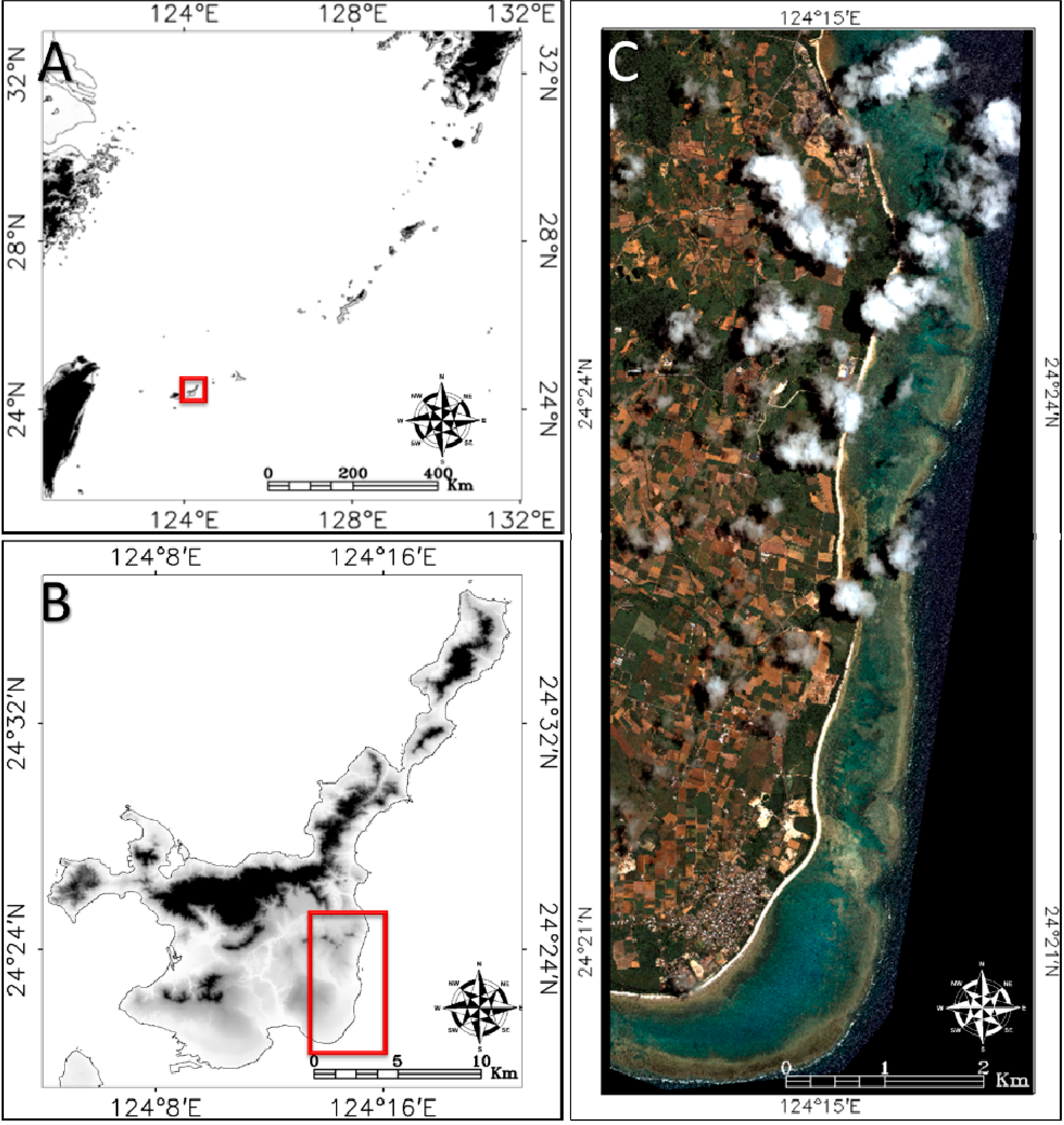
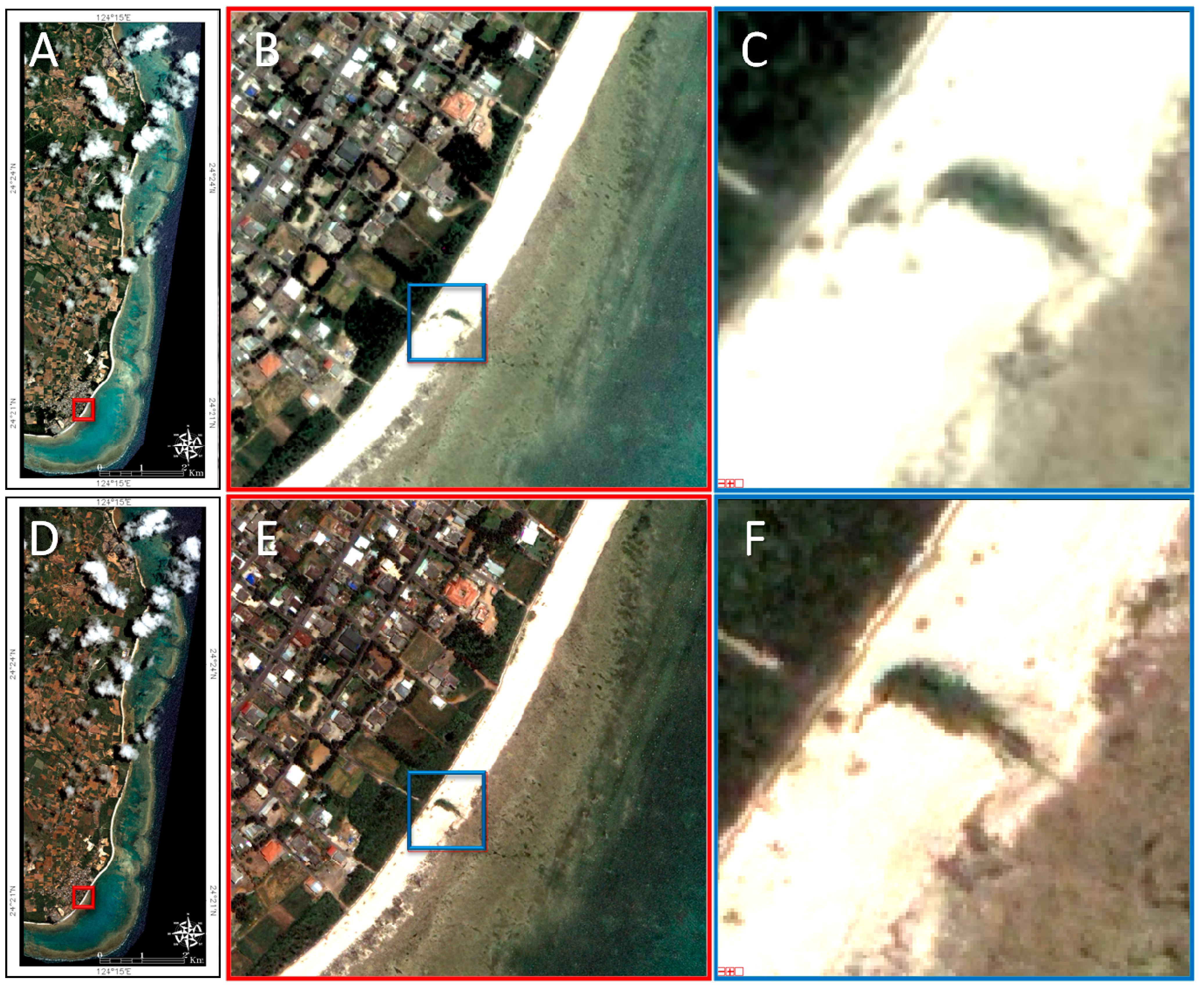
2.1. Study Site

Located at the extreme southwest of the Japanese Archipelago, Ishigaki Island lies on the 1200 km Ryukyu Arc, which has coasts featuring coral reefs and terraces of emergent coral reefs. Ishigaki coastal waters benefit from the strong western boundary Kuroshio Current, which connects the Philippine Sea tropical waters to the East China Sea subtropical waters [23]. Specifically, the Shiraho area hosts a rich marine biodiversity that includes three pivotal blue carbon ecosystems (i.e., mangroves, seagrasses and coral reefs), fish species, and the world’s largest colony of rare blue ridge coral (Heliopora coerulea). The area has been in a recovery phase since a severe bleaching occurred in 1998 [24] that caused a significant loss of healthy corals in Japan’s reefs, e.g., [25]; this ecological hotspot is now coping with soil runoff and sedimentation stemming from the increased number of farmlands in the adjacent watershed (Todoroki watershed). In addition to the reefscape with a well-developed reef (outer reef, reef crest, channels and moat) that includes intricate patches of branching (Acropora spp.) and massive (Porites spp., Heliopora coerulea) coral and seagrass, the Shiraho watershed shows a rural landscape composed of human infrastructure (buildings and roads) clusters, crop fields (sugarcane, bare soil) and grassland matrices as well as woodland compact areas. The high degree of landscape diversity and heterogeneity encountered across Shiraho’s seamless coast makes it suitable as the target area of our mapping.

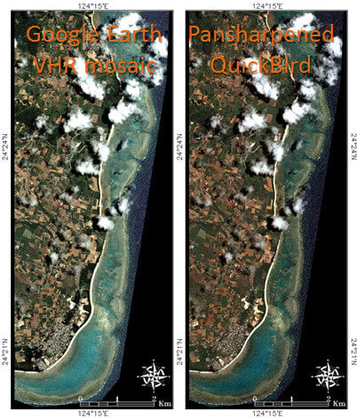
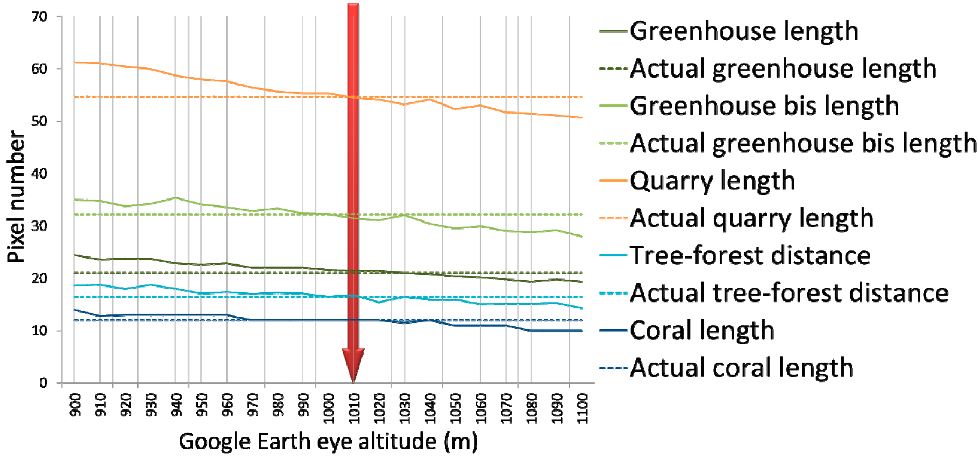
2.2. Remotely Sensed Datasets

Unlike the freely available license, the GE professional license ($US 399 per year) authorizes displayed RGB images (8-bit radiometric resolution) to be saved in the form of a Premium uncompressed JPEG file (4800 × 4153 pixels) with no copyright watermarks precluding any informational mapping. The construction of the GE spatial dataset relies on successive steps that can be summarized in a flowchart (Figure 2).
Figure 2. Conceptual flowchart describing the successive steps enabling a Google Earth-derived very high resolution mosaic to be created.
Ijgi 03 01157 g002
(1) Once the area of interest (ranging from local to regional scales) has been selected on GE (here, 44 km2 Shiraho area), an acquisition date should be specified (here, 2 July 2007) using the historical imagery button included in the GE toolbar. (2) Embedded at the bottom of the image is the company name of the source sensor (here, DigitalGlobe) following “Image © year”. DigitalGlobe provides high resolution multispectral satellite images (IKONOS, QuickBird, GeoEye-1 and WorldView-2, launched in 1999, 2001, 2008 and 2009, respectively). Although unstated, the sensor can be revealed (here, QuickBird, QB) based on the acquisition and sensor launch dates as well as the on-line DigitalGlobe and GeoEye archive browsers (browse.digitalglobe.com and geofuse.geoeye.com, respectively). Using the acquisition date over the targeted area, a series of image parameters such as the sensor vehicle, area maximum and average off nadir angles, average target azimuth, and area minimum sun elevation, can be freely retrieved. Because the sun elevation is correlated with the time at a specific date at a specific location, it is possible to compute the acquisition time (here, 02:45 Greenwich Mean Time, GMT) using a free on-line solar calculator (e.g., http://www.esrl.noaa.gov/gmd/grad/solcalc/), which is significant for deducing the tide level. (3) Positioning the virtual GE eye at the proper altitude and geometry are the next critical points. A preliminary analysis is based on the pixel measurements of five coastal features lying on the 0.6 m pixel size QB image (dotted lines in Figure 3) and the GE images gradually saved along an eye altitude gradient ranging from 900–1100 m (solid lines in Figure 3). Insofar as the confluence between the dotted and solid lines (see Figure 3) reveals the eye altitude at which the GE pixel size matches this of QB for each feature, the 1010 m eye altitude reaches consensus for the five features. (4) It is then possible to establish an acquisition plan over the area of interest that accounts for the appropriate eye altitude and an overlap of at least 30% between contiguous images. (5) Along the flight plan, it is especially important to carefully adjust the eye altitude with the drag slider, click “N” on the compass to set the yaw to north and position the field of view at nadir using the pitch control on the same compass. (6) After collecting all of the VHR images (here, n = 39), a mosaic procedure is performed that is facilitated by the substantial overlap among images. The free trial version of the bioimage Mayachitra Imago software (Mayachitra Inc., Santa Barbara, CA, USA) enabled the RGB images to be mosaicked based on the rotation-scaling-translation (RST) algorithm [26], which aligned the images by transforming the input images (neither stretching nor skewing) to optimally match the overlapping three-dimensional data. (7) The resulting VHR RGB mosaic is registered (RST warping and nearest-neighbor resampling, RMSE < 0.6) using the freely available QGIS software (qgis.org) based on ground control points (GCP) (here, n = 45, see red flags in Figure 4C) whose geographic coordinates are directly based on GE geolocations (geographic latitude/longitude projection and 1984 World Geodetic System (WGS84) datum) at the lowest eye altitude, which provides the greatest accuracy possible (i.e., 7 m) (Figure 4A). Importantly, the mosaicking procedure may be carried out freely during the 30 days of the Mayachitra Imago trial version, and would then cost from $US 200 to 1500 for a student and an academic license, respectively. Alternatively, the step 6 may be skipped and the step 7 may be applied to each image so that a final mosaic of registered images can be obtained.
Figure 3. Curve plot linking the Google Earth eye altitude and pixel number characterizing certain coastal targets of reference. The dotted lines correspond to the actual pixel number of each target of reference, measured on the QuickBird image, and the solid lines correspond to the targets’ pixel number derived from the Google Earth images saved along the 900–1100 m eye altitude range.
Ijgi 03 01157 g003
To assess the potential of GE for studying VHR coastal mapping, the exactly corresponding QB imagery collected on 2 July 2007 at 2:45 GMT over the Shiraho area was purchased. The 8-bit imagery is composed of four multispectral images (blue, green, red and infrared) at 2.4 m spatial resolution and one panchromatic image at 0.6 m spatial resolution. The spatial resolution of the multispectral images can be scaled up to the resolution of the panchromatic using the pixel-level fusion technique pansharpening [27]. Based on previous results [14], this procedure was applied using a simulation of the 2.4 m panchromatic image that accounts for the optical transmittance of the QB sensor, Gram-Schmidt sharpening transformation, and cubic convolution resampling. As a result, the source dataset featured RGB images (deletion of the infrared) with 0.6 m spatial resolution, thus paralleling those of GE. Initially referencing the UTM 52 N projection, the source dataset was further registered (RST warping and nearest-neighbor resampling) based on the previous 45 GCP (RMSE < 0.6) under the geographic latitude/longitude projection (Figure 4B).
Because of concerns regarding transferability, we processed the GE and source datasets directly from digital numbers (DN) without radiometric (radiance and reflectance) or sun-glint corrections. Clouds and their resulting shadows were masked out using a pre-classification resulting from an analysis-based visual delineation (Figure 4C).
Figure 4. Natural-colored (RGB) images of the study site stemming from (A) Google Earth-derived very high resolution mosaic and (B) QuickBird pansharpened imagery. (C) Natural-colored image of the study site overlaid by ground-truth locations: red flags symbolize the locations of the 45 ground control points; blue squares (n = 1005) and circles (n = 495) represent marine training and validation points, respectively, and green squares (n = 737) and circles (n = 363) represent the land training and validation points, respectively; yellow dots represent the location of the 22,481 acoustic measurements. (D) Mask image of the clouds (in red) and related shadows (in green).
Ijgi 03 01157 g004

2.3. Coastal Water Depth and Cover Types

Fieldwork data were collected (Figure 4C) for the water depth retrieval and marine and terrestrial mapping from 25–31 January 2013 and used as validation data for the remotely sensed images. Because the campaign was conducted five-and-a-half years after the satellite acquisition, a rigorous correction of the tide level for both the sonar survey and the satellite image enabled the surveyed and image-derived water depth to be compared on the same basis. Since there was no major high-energy event, such as a tsunami or strong typhoon, to damage the Shiraho area and no bleaching episode threatening the dominance of coral reefs, we may reasonably assume a socio-ecological spatial stability (i.e., no critical shifts in both human and natural habitats) during the satellite-to-field period. The seasonality effect will be further discussed.

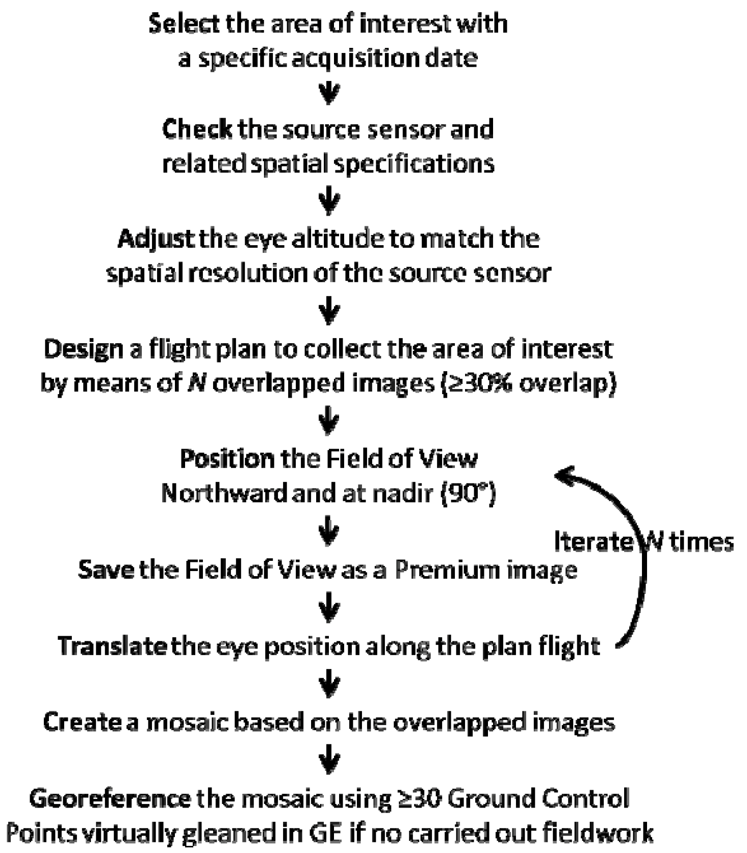
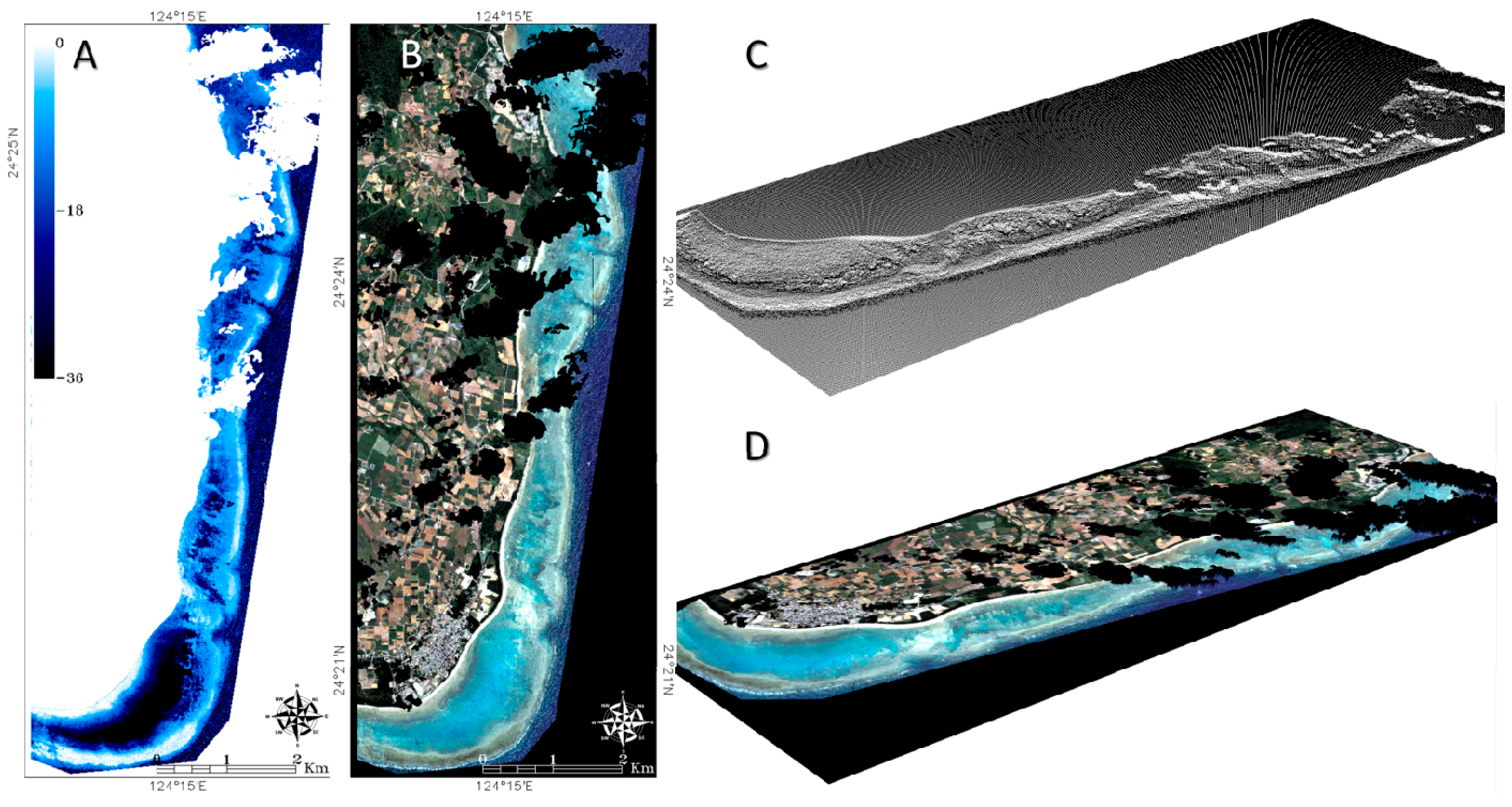
2.3.1. Bathymetry and Topography

An acoustic survey was conducted to measure the water depth of the Shiraho lagoon area. Sounding was performed from a small fishing boat equipped with a dual frequency (50/200 kHz) transducer (single beam) and 12-channel GPS antenna (Lowrance LCX-15MT). Data were recorded at 1 Hz to a multimedia card (MMC), and the boat followed transects across the lagoon at an average speed of 1 m∙s−1 and spanned a large variability of water depth and seabed cover. The horizontal and vertical spatial accuracy delivered by the acoustic system were estimated to reach 1 m and 0.03 m, respectively [28]. A total of 22,481 individual measurements were recorded and corrected for the tide level by coupling the GMT and Ishigaki Port tide prediction heights. (http://www1.kaiho.mlit.go.jp/KANKYO/TIDE/tide_pred/index_e.htm). The corrected dataset will assist in the quantification of the accuracy of further Digital Relative Depth Models (DRDMs).
To compute a DRDM using a simple but proficient methodology based only on RGB images, we opted for the calibrated ratio transform [29,30], solving for the water depth as follows:
z = m 1 ln ( n D N i ) ln ( n D N j ) m 0
where DNi and DNj refer to the digital numbers of the wavebands i and j, respectively; m1 and m0 are the slope and intercept of the fitted linear model; n is a fixed constant to ensure that the natural logarithm is positive. According to the increasing absorption of light by water from the blue to red bands, we tested three possible spectral combinations for each remotely sensed dataset. The resulting six DRDM were compared with the water depth measurements and specifically corrected for the tide level bound to the satellite acquisition time. The accuracy of the DRDM was determined by computing the Pearson product-moment correlation coefficient (r) and coefficient of determination related to the fitted linear model (R2). The comparison of the DRDM accuracy was performed to show the significance of the differences using the following equation:
Z = | R i 2 × N i N i R j 2 × N j N j | ( R i 2 × N i + R j 2 × N j ) ( N i + N j ) × ( 1 ( R i 2 × N i + R j 2 × N j ) ( N i + N j ) ) × ( 1 N i + 1 N j )
where Ri2 and Rj2 refer to the linear coefficients (determining the relationships between modeled and actual water depths) pertaining to DRDM i and DRDM j, respectively; and Ni and Nj correspond to the total amount of soundings over the DRDM i and DRDM j, respectively. Because of the large sample size and central limit theorem, the value Z can be confidently used to test the significance level between two DRDM because the Z distribution can be approximated by a normal distribution under the null hypothesis.
Topographical data, which were not derived from the remotely sensed datasets, were employed to verify whether it improves the mapping results associated with terrestrial cover types. For the sake of affordability, freely available elevation data were sourced from the Advanced Spaceborne Thermal Emission And Reflection Radiometer (ASTER) Global Digital Elevation Model (GDEM) Version 2, provided at one arcsecond (approximately 30 m at the equator) and 8 m of horizontal and vertical resolution (http://www.jspacesystems.or.jp/ersdac/GDEM/E/4.html). A digital elevation model scaled up at 0.6 m spatial resolution was created by interpolating to regular grid Delaunay-triangulated GDEM data points (Figure 5A). A relevant combination of the GDEM and GE natural-colored (Figure 5B) data consists of calculating an elevation-based 3D point cloud (Figure 5C) over which the GE image can be draped (Figure 5D).
Figure 5. Maps of the (A) elevation and (B) natural-colored (RGB) data over the study site stemming from Global Digital Elevation Model Version 2 and Google Earth-derived very high resolution mosaic, respectively. Based on xyz data, (C) a 3D point cloud was built, over which the RGB image was draped (D).
Ijgi 03 01157 g005

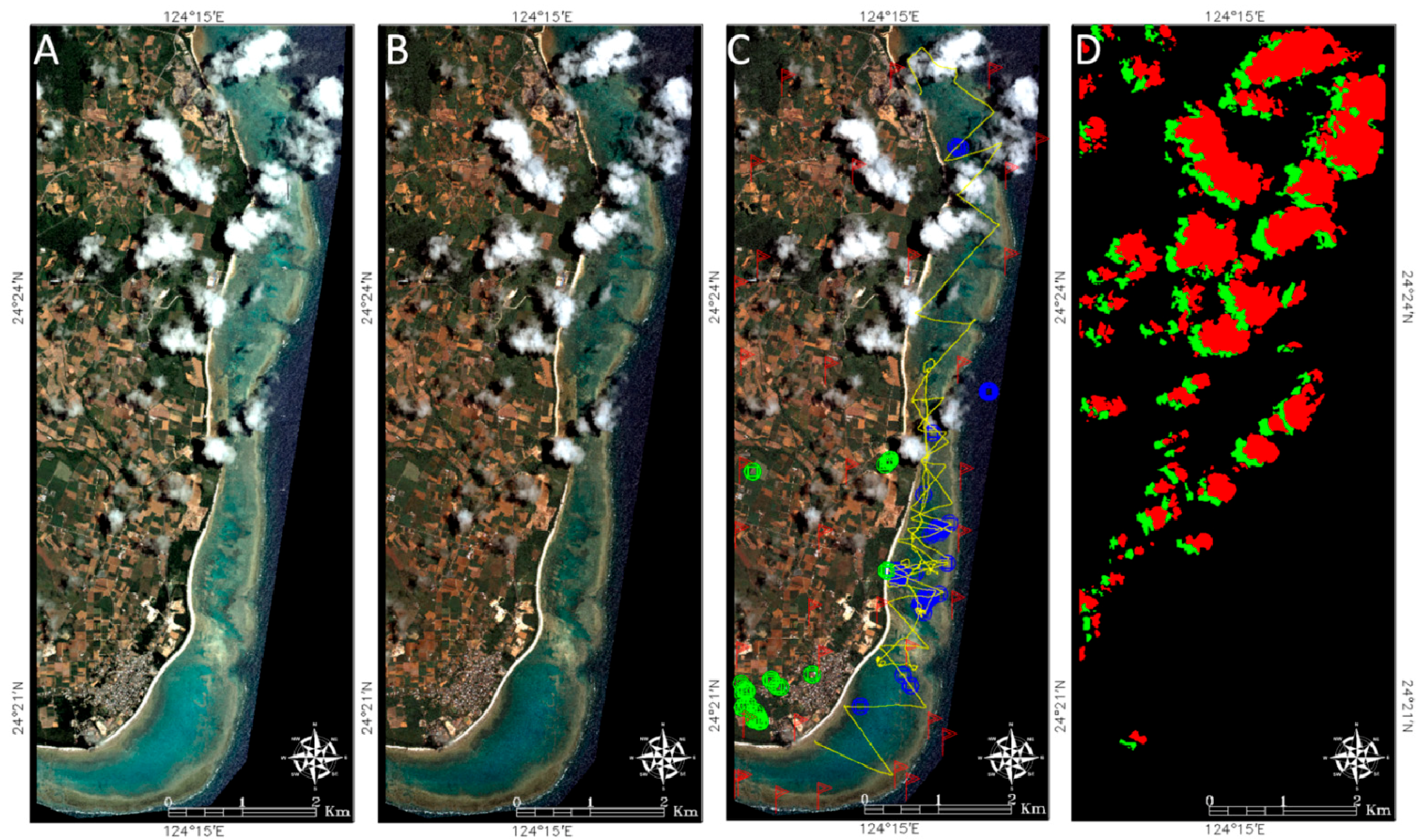
2.3.2. Coastal Cover Types

Because of the required level of precision, the collection of marine images was conducted simultaneously with the sonar survey and determination of terrestrial cover types was undertaken using local knowledge of the area and image inspection.
Underwater images were acquired from a low-cost compact high resolution video camcorder (GoPro Hero 3, 1440 res, 30 fps with wide field of view) placed just underneath the water surface so that very shallow seabeds could be monitored. An array of 7h54min50s video recordings that were geolocated with 1 m horizontal accuracy (see sonar survey) enabled the extraction and further analysis of 166 high-quality images. A grid of 100 evenly distributed cases was superimposed on each image to quantify the surface area occupied by various seabed types (n = 15, Table 1). Relying on the percentage of dominant seabed type (>90%), 10 so-called pure images by seabed type were selected and considered as representatives of their inherent type. By matching the locations of the pure images and corresponding pixels, a spectrally even buffer area was grown around each pixel so that a series of 100 pixels was assigned to each seabed type.
Land reference data were composed of a mix of in situ georeferencing and image interpretation. A panel of 11 land types (Table 1) was selected as the representative cover types in Shiraho. For sparse but noteworthy types, such as sugar cane fields and mangrove forests, the geographic coordinates of the target perimeter were attained using a handheld Garmin eTrex 20 GPS. For sufficiently contrasted spatial and spectral information, the pixels tied to the remaining land types (n = 9, Table 1) were assigned through a visual inspection by a single analyst. For each land type, 100 pixels were selected either between or around the core pixels (i.e., matching locations of the surveyed and mapped data) to determine a dataset that is balanced within a seamless coastal landscape.
Table 1. Description of the 26 seamless coastal cover types in Shiraho, which contain 15 marine and 11 terrestrial classes.
RealmCover TypeDescription
MarineAbenthicOptical deep water
MudTerrigeneous and coralligeneous clastic sediment below 0.0625 mm grain size
Fine sandCoralligeneous clastic sediment ranging from 0.0625 to 0.25 mm grain size
SandCoralligeneous clastic sediment ranging from 0. 25 to 0.5 mm grain size
Coarse sandCoralligeneous clastic sediment ranging from 0.5 to 2 mm grain size
PebbleCoralligeneous clastic sediment ranging from 2 to 64 mm grain size
CobbleCoralligeneous clastic sediment ranging from 64 to 256 mm grain size
BoulderCoralligeneous clastic sediment ranging above 256 mm grain size
Blue algaeCyanobacteria communities eroding consolidated coralligeneous sediment
Brown algaeTufts or carpets of macroalgae dominated by Turbinaria spp. and Padinae spp.
Calcareous algaeEncrusting algae communities (e.g., coralline) eroding consolidated coralligeneous sediment
SeagrassMeadows of aquatic phanerogam composed of Cymodocea sp., Halodule sp., Halophila sp., Zostera japonica
Hard coral bommiePseudo-spherical massive coral colony dominated by hexacorallian Porites spp.
Hard coral thicketField of thicket coral colony dominated by hexacorallian Acropora spp.
Blue coralPseudo-spherical massive coral colony dominated by octocorallian Heliopora coerulea
TerrestrialRiverElongated inland water body
Wet sandIntertidal coralligeneous clastic sediment ranging from 0.0625 to 2 mm grain size
Dry sandSupratidal coralligeneous clastic sediment ranging from 0.0625 to 2 mm grain size
SoilVarious bare substrata devoid of vegetation (if any, very sparse)
GrassNatural and mowed herbaceous (≤0.5 m) poaceae communities
Crop fieldCultivated herbaceous vegetables and fruits
Sugar cane fieldCultivated shrub poaceae (≥0.5 and ≤6 m)
Mangrove forestNatural mix of shrubs and trees (≥6 m) rhizophoraceae
Dark forestNatural mix of tree aquifoliaceae dominated by Ardisia quinquegona
RoadAnthropogenic infrastructure characterized by asphalt-covered curve lines
RoofAnthropogenic infrastructure made of ceramic or metallic tiles

2.3.3. Classification of Coastal Covers and Accuracy Assessment

The classification of the study area was performed for each of the remotely sensed datasets to test the reliability of GE for coastal mapping. Ground-truth pixels characterizing the 26 classes were divided into two independent clusters: the training cluster, which helped define the class-specific spectral signatures required for classification, and validation cluster, which was used to assess the accuracy of the classification process. Out of the 100 pixels representative of each class, 67 and 33 were randomly attributed to the training and validation clusters, respectively. The widely spread maximum likelihood (ML) algorithm (QGIS) is a pixel-based, supervised procedure fueled by the 67 pixels of the 26 classes. Prior to launching the ML classifier, a curve boundary separating the land from water was manually delineated over the wet/dry sand demarcation line. The ML procedure was conducted over a marine area devoid of land based on the RGB and RGB + bathymetry datasets and was also applied over a terrestrial area devoid of sea based on the RGB and RGB + topography datasets.
The validation cluster was required to construct a confusion matrix so that the accuracy of each classification (n = 8) could be quantified. This technique relies on the proportion of pixels that are correctly classified in the resulting image based on the match between the class identity of the validation and classified pixels. Four indicators synthesize the results of the confusion matrix: the overall accuracy (OA), kappa coefficient (κ), producer’s accuracy (PA) and user’s accuracy (UA). OA is determined by dividing the total number of correctly classified pixels by the total number of validation pixels (i.e., diagonal of the confusion matrix), whereas κ provides a single proportion of accuracy agreement above that of a random assignment of classes (i.e., off-diagonal of the confusion matrix). PA (omission error) and UA (commission error) determine the percentage of correct predictions for each coastal class [31]. A comparison between the classification accuracies was conducted to underscore the significance of the differences using the following equation:
Z = | C i N i C j N j | ( C i + C j ) ( N i + N j ) × ( 1 ( C i + C j ) ( N i + N j ) ) × ( 1 N i + 1 N j )
where Ci and Cj refer to the correctly classified pixels pertaining to Classification i and Classification j, respectively; and Ni and Nj correspond to the total amount of validation pixels across the Classification i and Classification j, respectively. Because of the large sample size and central limit theorem, the value Z can confidently be used to test the significance level between two classifications because the Z distribution can be approximated by a normal distribution under the null hypothesis. A two-tailed test was used to compute the statistical significance.

3. Results

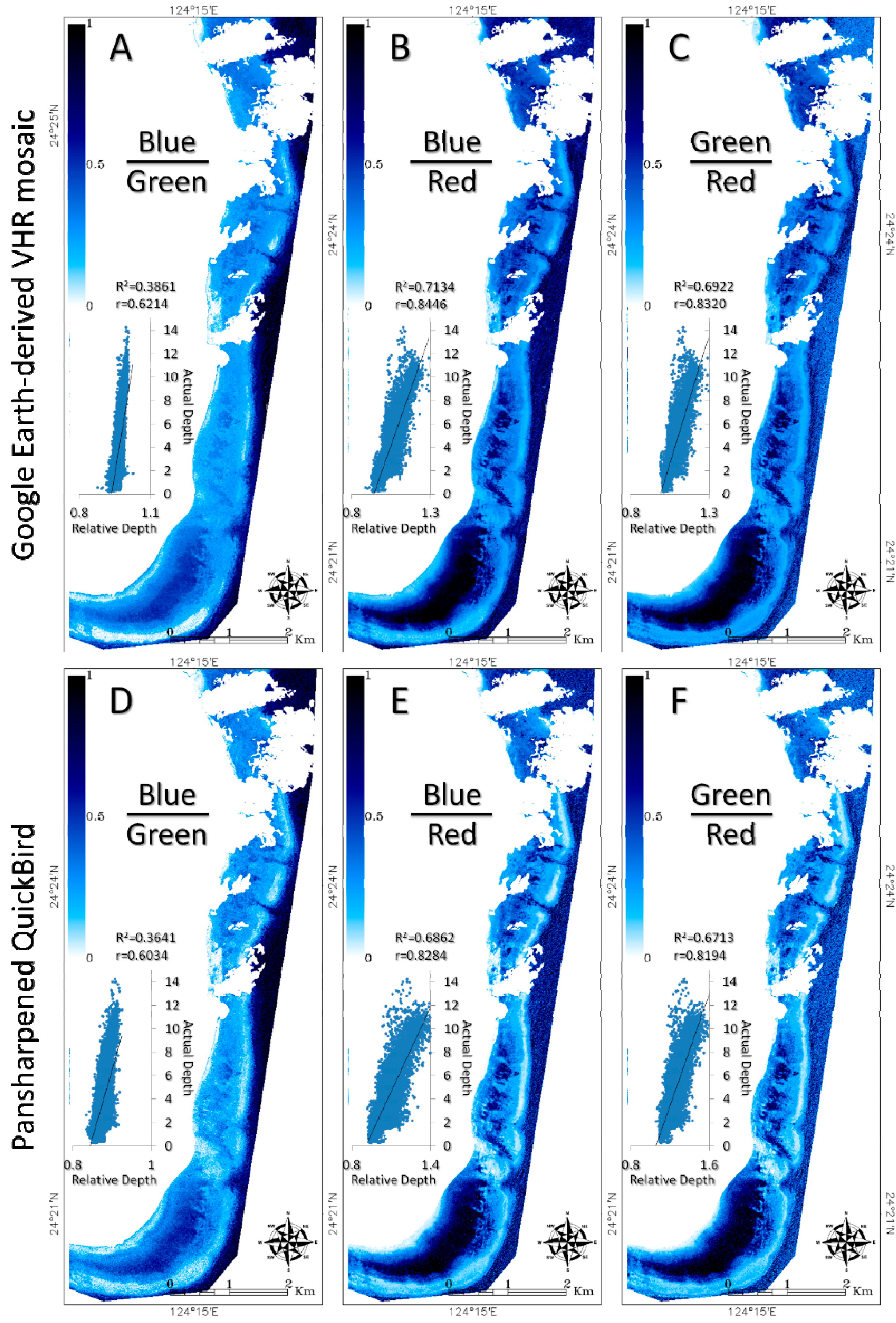
3.1. Comparison of the Water Depth Retrieval

Using the uncalibrated ratio transform, three Digital Relative Depth Models (DRDM) were produced for both the Google Earth (GE)-derived very high resolution (VHR) mosaic and pansharpened QuickBird (QB) imagery (Figure 6). For both datasets, the ratio transforms involving the blue and red spectral bands (see Figure 6B,E) were closely followed by the green-red combination (see Figure 6C,F) and provided satisfactory measures of agreement between the modeled and actual water depths (R2 ≈ 0.69). Interestingly, the blue-red combination (most accurate) reached higher measures of agreement for GE compared to QB (R2GE = 0.7134 versus R2QB = 0.6862, Z = 6.29, αtwo-tailed < 0.002). This performance difference between GE and QB occurred systematically in favor of GE across the three ratio transforms (Table 2). For both datasets, the blue-red DRDM were calibrated to a digital depth model (DDM) using the linear fitting model (associated with the R2 value indicated in Figure 6B,E) to test whether and the extent to which the seabed mapping may be improved by merging the DDM to RGB bands.
Figure 6. Digital Relative Depth Models (DRDM) resulting from the ratio transform based on blue-green, blue-red and green-red spectral bands derived from (A, B and C, respectively) Google Earth-derived very high resolution mosaic imagery and (D, E and F, respectively) pansharpened QuickBird imagery. Scatterplots comparing the relative and actual depths as well as the linear coefficient of determination (R2) and Pearson product-moment correlation coefficient (r) are embedded for each DRDM.
Ijgi 03 01157 g006
Table 2. Compilation of the Z-values between the three Digital Relative Depth Models with respect to the Google Earth-derived very high resolution mosaic and pansharpened QuickBird imagery.
Google EarthQuickBird
Blue/GreenBlue/RedGreen/RedBlue/GreenBlue/RedGreen/Red
Google EarthBlue/GreenX69.7465.104.82NCNC
Blue/Red69.74X4.92NC6.29NC
Green/Red65.104.92XNCNC4.76
QuickBirdBlue/Green4.82NCNCX68.3865.18
Blue/RedNC6.29NC68.38X3.38
Green/RedNCNC4.7665.183.38X
Notes: NC means non-computed because of the purpose of the study.
Mimicking the elevation-related Figure 5, the calibrated DDM (Figure 7A) may be exploited to create a 3D point cloud (Figure 7C) over which the GE natural-colored image (Figure 7B) can be draped (Figure 7D).
Figure 7. Maps of the (A) water depth and (B) natural-colored (RGB) data over the study site stemming from the Google Earth (GE) blue-red ratio transform and GE-derived very high resolution mosaic, respectively. Based on xyz data, (C) a 3D point cloud was constructed, over which the RGB image can be draped (D).
Ijgi 03 01157 g007

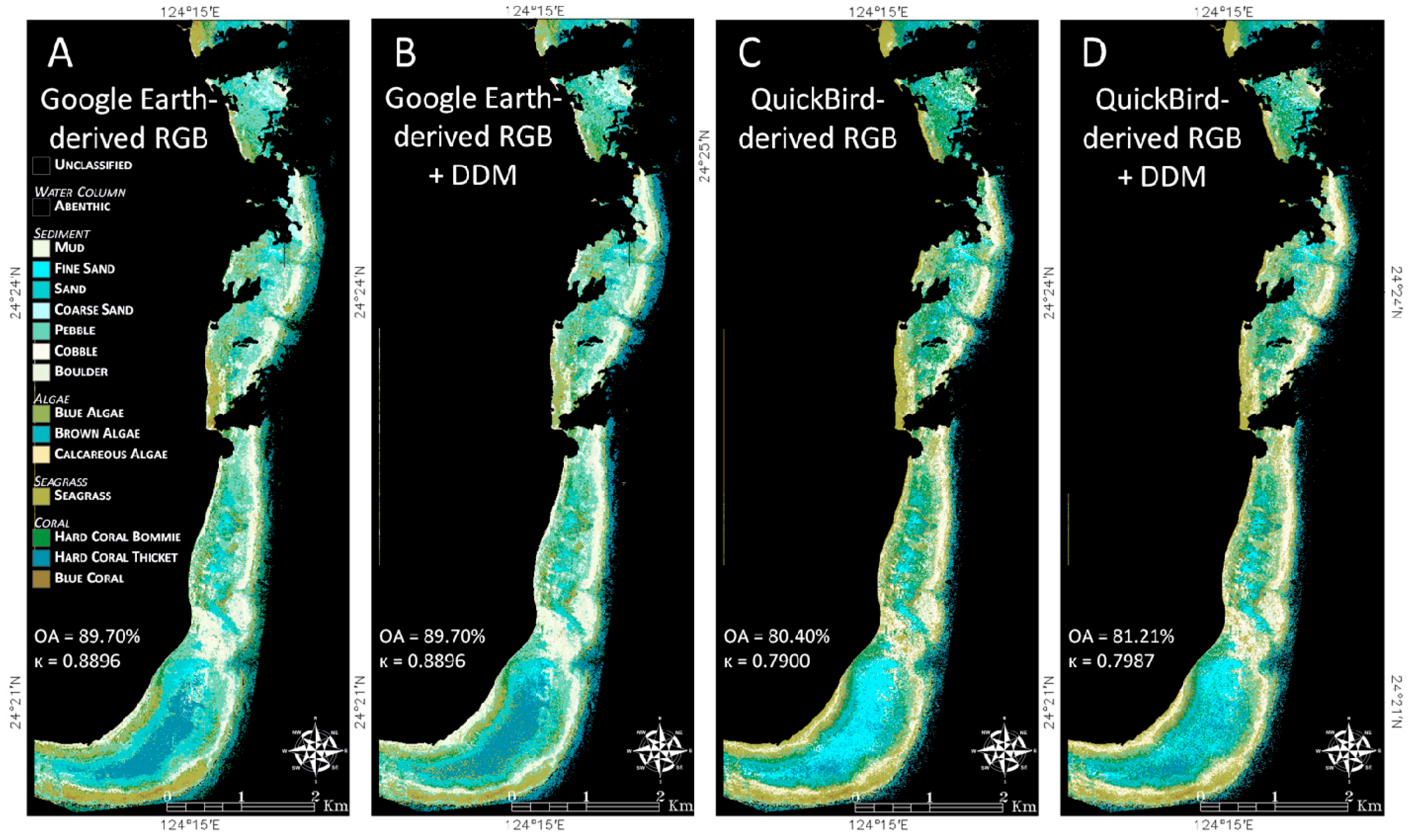
3.2. Comparison of the Seabed Cover Mapping

The marine portion of the study area was classified into 15 classes for both the GE-derived VHR mosaic and pansharpened QB imagery, which were devoid of and provided with the associated DDM (Figure 8). Satisfactory to very satisfactory overall accuracies (OA) ranging from 80%–90% were found for all of the datasets, and the GE-derived seabed maps were better matched to the validation data than those stemming from QB (OAGE = 89.70% versus OAQB = 80.40%, Z = 4.10, αtwo-tailed < 0.002). Although the GE-derived mapping displayed no UA and a single PA below 60% (i.e., PASeagrass = 57.58%), QB-related accuracies below 60% included two UAs (UASeagrass = 58.33% and UABlue coral = 55.56%) and two PAs, of which the seagrass attained a very low performance (PAHard coral bommie = 54.55% and PASeagrass = 21.21%) (Table 3). Including the water depth data with the RGB datasets, did not modify the GE-derived OA (OAGE = 89.70%) and slightly but insignificantly improved the QB-derived OA (from OAQB = 80.40% to OAQB_DDM = 81.21%, Z = 0.32, αtwo-tailed = 0.749). Despite the unchanged OA, the water depth information produced permutations among the GE-derived UA and PA that were beneficial to seagrass (PA = +15.15%) and all three of the coral classes (PAHard coral bommie = +18.18%, UAHard coral thicket = +15.25%, UABlue coral = +10.88%) and detrimental to mud (PA = −15.15%) and blue coral (UA = −10.22%). The modest improvement of QB mapping by including the water depth data appeared to be partly reflected by an enhanced seagrass discrimination (UA = +11.67%) as well as pebble discrimination (PA = +9.09% and UA = +9.02%).
Figure 8. Seabed cover maps (15 classes) resulting from the Google Earth-derived very high resolution mosaic (A) without and (B) with an inherent digital depth model (DDM), and from the pansharpened QuickBird imagery (C) without and (D) with an inherent DDM. For each map, the overall accuracy (OA) and kappa coefficient (κ) are overplotted.
Ijgi 03 01157 g008
Table 3. Producer’s accuracy (PA) and user’s accuracy (UA) of the 15 seabed cover types with respect to the RGB Google Earth-derived very high resolution mosaic, QuickBird pansharpened datasets, and digital depth model (DDM).
Google EarthQuickBird
RGBRGB + DDMRGBRGB + DDM
PAUAPAUAPAUAPAUA
Abenthic100100100100100100100100
Mud90.9110090.9183.3375.7692.5984.8587.5
Fine sand10010096.9710010010096.97100
Sand10010096.9796.9710097.0696.9794.12
Coarse sand10010010094.2910010010091.67
Pebble10010075.7660.9810097.0684.8570
Cobble10089.1984.8590.3290.9183.3384.8590.32
Boulder90.9110010094.2996.9794.1296.9794.12
Blue algae10097.0675.7665.7910086.8475.7660.98
Brown algae10010096.9796.9796.9710090.9193.75
Calcareous algae10094.2972.7377.4296.9791.4378.7974.29
Seagrass57.5861.2921.2158.3372.7366.6721.2170
Hard coral bommie63.647054.5566.6781.8277.1460.6168.97
Hard coral thicket66.6768.7578.7961.963.648478.7968.42
Blue coral75.7665.7960.6155.5669.776.6766.6757.89

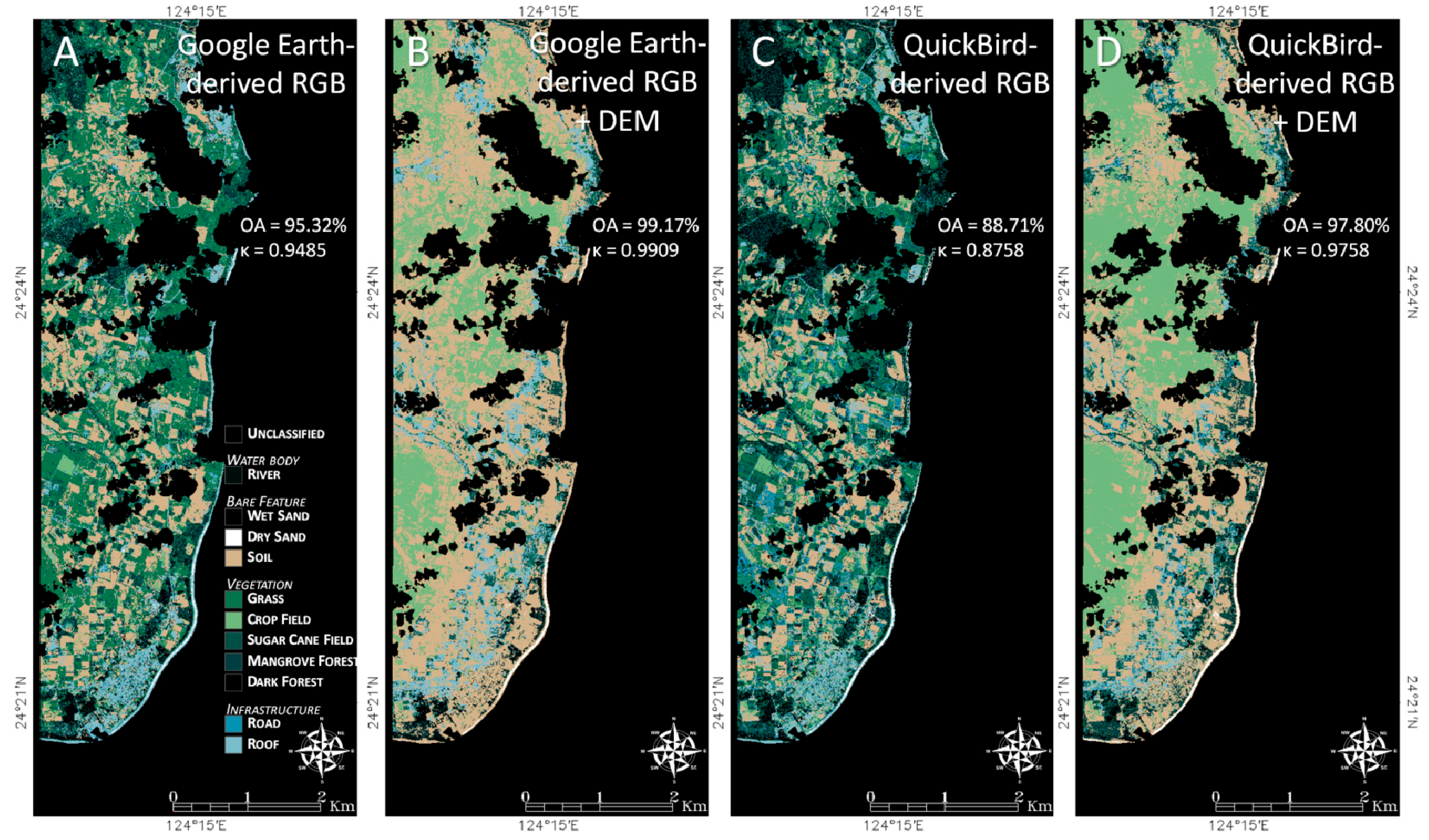
3.3. Comparison of the Land Cover Mapping

The land portion of the coastal area was categorized into 11 classes for both the GE-derived VHR mosaic and pansharpened QB imagery that were devoid of and provided with the associated DEM (Figure 9). Across the band modalities, the 11 targeted features benefited from a successful classification that spanned the highest deciles of both measures of agreement. Once again, the GE-based land maps produced better results than the corresponding QB-based maps (OAGE = 95.32% versus OAQB = 88.71%, Z = 3.28, αtwo-tailed < 0.002). Contrary to the GE RGB dataset, the QB dataset showed six UA and PA performing below 84%, of which one bottomed at 48.48% (PAMangrove forest) (Table 4). The combination of elevation information and RGB datasets significantly increased the GE and QB classification accuracy by 3.85% (OAGE_DEM = 99.17%, Z = 3.17, αtwo-tailed < 0.002) and 9.09% (OAQB_DEM = 97.80%, Z = 4.88, αtwo-tailed < 0.002), respectively. The inclusion of elevation was beneficial to the GE-mapped human infrastructure (PARoof = +12.12% and UARoad = +11.35%) and considerably improved the distinctness of the QB-related mangrove forest (PA = +51.52% and UA = +30.29%), dark forest (PA = +21.21% and UA = +23.53%), road (UA = +17.2%) and river (UA = +13.89%).
Figure 9. Land cover maps (11 classes) resulting from the Google Earth-derived very high resolution mosaic (A) without and (B) with an inherent digital elevation model (DEM) and from the pansharpened QuickBird imagery (C) without and (D) with an inherent DEM. For each map, the overall accuracy (OA) and kappa coefficient (κ) are overplotted.
Ijgi 03 01157 g009
Table 4. Producer’s accuracy (PA) and user’s accuracy (UA) of the 11 land cover types with respect to the RGB Google Earth-derived very high resolution mosaic, QuickBird pansharpened datasets, and digital elevation model (DEM).
Google EarthQuickBird
RGBRGB + DEMRGBRGB + DEM
PAUAPAUAPAUAPAUA
River87.8893.5596.9796.9793.9486.1193.94100
Wet sand10010010010096.97100100100
Dry sand93.94100100100100100100100
Soil10010010010093.9496.8896.9794.12
Grass10097.0610010090.9190.91100100
Crop field10010010010010094.2993.94100
Sugar cane field96.9710010010010094.29100100
Mangrove forest96.9788.8996.9796.9748.486410094.29
Dark forest96.9791.4310010078.7976.47100100
Road90.9185.7110097.0690.9176.9296.9794.12
Roof84.8593.3396.9710081.8293.193.9493.94

4. Discussion

4.1. Coastal Shallow Water Depth

Both GE- and QB-based water depth retrievals within Shiraho marine zones ranging from 0–15 m reached a satisfactory measure of agreement with the acoustic survey (R2 ≈ 0.7). It is noteworthy that the sounding survey occurred along the lagoon and not along the deeper outer reef (see yellow lines in Figure 4C). In addition, the survey coverage contained some along-shore lines which may exaggerate the water depth accuracy in overweighting some water depth ranges. The measure of agreement, however, corroborates the research works using VHR multispectral spaceborne data and the eight-band WorldView-2 sensor [30,32]. Regardless of the data source, the best water depth extraction was obtained from a combination of the blue and red bands and to a lesser extent by the green and red bands. This result may be explained by the difference in light absorption by water [33]. Although the difference in the blue and green coefficients of absorption is approximately 0.045 (= 0.065 − 0.02), the differences associated with both the blue-red and green-red coefficients reach 0.35 (= 0.37 − 0.02) and 0.305 (= 0.37 − 0.065), respectively [33]; greater differences produce a finer discrimination in the full-range of water depths. There is a significant lack of global water depth charts of coastal areas because their shallowness precludes the application of traditional waterborne surveys. The satisfactory water depth retrieval obtained from a combination of an acoustic survey and a GE professional license holds great promise for providing failsafe water depths at the submeter scale over local and regional extents. As a reflection of the synergistic collaboration between forest researchers and GE scientists [34], it would be highly relevant to apply the method described in this paper to coastal areas leveraging GE VHR data to assist researchers and stakeholders in addressing urgent coastal issues.
Based on a substantial sampling (NGE = 22,478 and NQB = 22,481), all of the accuracy measures were significantly distinct (αtwo-tailed < 0.002), and the three GE-based DRDM remarkably outperformed those of the QB (see Figure 6 and Table 2). These original findings are surprising because the GE-derived VHR mosaic is sourced from QB data that are provided with the exact same time and location. We previously indicated that the significant differences between the two datasets are a result of either a divergence in the image processing technique, such as the pansharpening procedure, image assimilation technique, such as the JPEG format conversion, or a combination of both factors. The visual examination of both datasets at the highest resolution reveals a segregation in the image texture (Figure 10). Although we applied the resampling technique to produce the smoothest results (cubic convolution, see [14]) in the QB pansharpening procedure, the variation of GE pixel values with distance is obviously lacking high spatial frequency compared to that of QB. Therefore, it is reasonable to assume that GE scientists have applied a customized pansharpening algorithm to QB images and assimilated the images in the form of JPEG files to yield smoother output VHR images and that this smoother image better matched the spatial accuracy of the acoustic survey (e.g., GPS horizontal accuracy). Other spectral sharpening methods, such as the Color Normalized or Principal Component algorithms, should be tested in order to elucidate the GE products.
Figure 10. Natural-colored (RGB) images of the entire study area, red square zoom-in and blue square zoom-in stemming from Google Earth-derived very high resolution mosaic (A, B and C, respectively) and from pansharpened QuickBird imagery (D, E and F, respectively).
Ijgi 03 01157 g010

4.2. Seamless Seabed and Land Cover Mapping

The coastal zone was successfully mapped in a seamless manner at a VHR by both GE and QB datasets, with approximately 26 cover types resolved and typified by a lowest OA equaling 80.40% (i.e., OAQB_Seabed). The very high classification accuracies have to be contextualized on the basis of the proximity of the ground-truth pixels. Although randomly sampled, the training and validation pixels may suffer from a spatial autocorrelation, incurring a likely overestimation of the accuracy. Both datasets were composed of the three blue, green and red bands (the infrared band was excluded) and overarched sufficiently rich spectral information to discriminate primary cover features in a spatially complex environment. Consistent with the water depth results, the findings related to the classification accuracy showed that the GE dataset produced more reliable coastal cover maps for both marine and terrestrial realms than did the QB dataset. Specifically, the hard coral bommie, blue coral, dark and mangrove forests were much better classified based on GE data than on QB data. Presupposing the GE-driven smoother texture image, we can hypothesize that the pansharpened QB imagery featured a texture sharp enough that the sun glint occurring over very shallow coral colonies and leaf-induced speckles over dense tree canopies impeded a robust classification.
The integration of freely available elevation data into the RGB GE and QB datasets significantly enhanced the land cover classification accuracy, particularly for (1) human infrastructure, (2) dark and mangrove forests and, to a lesser degree, roads and rivers, respectively. The GDEM is derived from the stereoscopic sensor ASTER, which captures and renders 3D landscapes that include cover features [35]. Consequently, the GDEM maps the top of the human infrastructure and tree canopies, which explains the greater classification consistency for land cover types demonstrated in our study. Despite the initial spatial resolution of one arcsecond, we recommend combining the GDEM-nested elevation data that are rasterized at the appropriate VHR with the RGB GE-derived mosaic to optimize the land cover mapping. However, including the water depth information retrieved from the RGB datasets to either of the datasets did not significantly improve the marine cover mapping. This result may be explained by the absence of a water column correction to account for the RGB light by water, which is intricately linked with the water depth. Ongoing research on the radiometric calibration of GE data that is based on the sensitivity of the source sensor and sun-scene-sensor trigonometry has a strong potential to provide water-leaving reflectances that are capable of retrieving seabed reflectances when merged with calibrated DDMs.

4.3. Limitations

The methodology developed and discussed in this study has certain computational, optical and data limitations.
The study area spanned 44 km2 and required 39 individual JPEG Premium files, which amounted to slightly less than one image per km2. After designing an ad hoc acquisition plan that may be constructed by a permanent visualization onto GE (e.g., 1 km gridlines), the standardized collection (see Section 2.2) of the 39 images may be relatively easy and fast. The main challenge resides in completing the mosaic, which is intricately linked with the joint capabilities of the inherent software and processor. Managing a coastal area greater than 50–100 km2 at VHR will therefore rely much more on the computational efforts to achieve a (very) large mosaic rather than on the image collection. One solution to this dilemma is to maintain the same number of images to be mosaicked but collect the images at higher GE eye altitudes so that the field of view can be extended, which would allow the mosaic to cover areas on the order of hundreds of km2. Bridging the values of GE eye altitude with those of all of the VHR and HR instruments’ multispectral and panchromatic pixel sizes is an objective that is being currently addressed.
This study directly and indirectly compares the mapping results derived from QB through the GE filtering. The infrared band was excluded from the purchased QB for the sake of comparison. Because of the significant reflection and absorption of the infrared light by vegetation and water, respectively, the discrimination power of QB on land cover is susceptible to be augmented, but very little on seabed cover. The radiometric resolution of the purchased QB was resampled at 8 bits to parallel the JPEG-converted GE images; this process facilitated the interpretation of the results. Nevertheless, QB and new VHR sensors (see Section 2.2) provide spatial data with 11-bit radiometric resolution. Because of the exponential increase in the dynamic range (from 256–2048 digital numbers per spectral band), the mapping performance of the purchased images is likely to increase. The well-documented GE predominance over source 8-bit images, which was demonstrated in this paper, must be examined against 11-bit images. Contrary to QB, the GE images based on digital numbers do not benefit from metadata allowing images to be radiometrically calibrated and atmospherically corrected. This lack may seriously hinder or jeopardize the water depth and cover mapping over areas featured by, for instance, a high level of evaporation. Tackling this paucity of information using freely available on-line metadata is a critical ongoing research, as evoked in Section 4.2.
The Shiraho coastal area located along the southeastern area of the Ishigaki Island embodies a well-studied coastal area (mainly because of its coral reefs) in Japan and hosts a high number of researchers who can afford commercial VHR images. Consequently, DigitalGlobe has programmed image acquisitions over the Shiraho area that now leverage five VHR images from 2007–2012, which are available on GE. The availability of VHR images is closely related to the provider’s effort in acquiring data, which in turn is dependent on the ability of the customer to pay for such images. This assertion is consistent with that of a study of the horizontal positional accuracy over 109 cities worldwide, which showed a significant difference between developed and developing countries at the expense of the latter [21]. Prior to selecting a study area for analysis by our methodology, it is strongly recommended to consult the GE historical imagery to help determine the feasibility of studies on coastal landscape dynamics. The very low PA related to the seagrass classification may arouse some interrogations about a winter-summer effect. We therefore want to draw attention on a potential seasonality likely to bias the classification accuracy of some habitats, especially those provided with chlorophyll.

5. Conclusions

Focused on the seamless coastal area of Shiraho (Ishigaki, Japan), we found that both RGB GE-derived mosaic imagery and RGB pansharpened QB imagery yielded satisfactory to very satisfactory results for the water depth (R2GE = 0.71 and R2QB = 0.69), seabed cover (OAGE = 89.70% and OAQB = 80.40%, n = 15 classes) and land cover (OAGE = 95.32% and OAQB = 88.71%, n = 11 classes) mapping. In addition, we showed for the first time that the GE dataset significantly outperformed the QB dataset for all three mappings (ZWater depth = 6.29, ZSeabed = 4.10, ZLand = 3.28, αtwo-tailed < 0.002). The integration of freely available elevation (GDEM) data into both RGB datasets significantly improved the land cover classification accuracy (OAGE = 99.17% and OAQB = 97.80%) compared to that of the water depth. Because of the associated easy-to-transfer methodology described in this paper, GE data might be an inexpensive alternative for researchers and stakeholders tasked with coastal management over worldwide coastal areas that are provided with VHR coverage.

Acknowledgments

This study was fully supported by Grant-in-Aid for JSPS Fellows (No. 2402800) of the Japan Society of the Promotion of Science (JSPS) and partly supported by Grant-in-Aid for Scientific Research (A) (No. 24246086, 25257305) of JSPS. The first author also acknowledges Hiroyuki Takamiyagi, who nimbly drove the boat along the full-range of lagoon water depths. This paper was significantly improved by the comments and suggestions of two reviewers who neatly underlined points to be clarified and contextualized.

Author Contributions

These authors contributed equally to this work.

Conflicts of Interest

The authors declare no conflict of interest.

References

  1. Costanza, R.; d’Arge, R.; de Groot, R.; Farber, S.; Grasso, M.; Hannon, B.; Limburg, K.; Naeem, S.; O’Neill, R.V.; Paruelo, J.; et al. The value of the world’s ecosystem services and natural capital. Ecol. Econ. 1998, 25, 3–15. [Google Scholar] [CrossRef]
  2. Sukhdev, P. The Economics of Ecosystems and Biodiversity; European Communities: Wesseling, Germany, 2008. [Google Scholar]
  3. The Other 70% UNEP Marine and Coastal Strategy; UN-Gigiri: Nairobi, Kenya, 2011.
  4. Martínez, M.L.; Intralawan, A.; Vázquez, G.; Pérez-Maqueo, O.; Sutton, P.; Landgrave, R. The coasts of our world: Ecological, economic and social importance. Ecol. Econ. 2007, 63, 254–272. [Google Scholar] [CrossRef]
  5. Intergovernmental Panel on Climate Change (IPCC). Climate Change 2013—The Physical Science Basis: Working Group I Contribution to the Fifth Assessment Report of the Intergovernmental Panel on Climate Change; Stocker, T.F., Qin, D., Plattner, G.K., Tignor, M., Allen, S.K., Boschung, J., Nauels, A., Xia, Y., Bex, V., Midgely, P.M., Eds.; Cambridge University Press: Cambridge, UK, 2013. [Google Scholar]
  6. Adger, W.N.; Hughes, T.P.; Folke, C.; Carpenter, S.R.; Rockström, J. Social-ecological resilience to coastal disasters. Science 2005, 309, 1036–1039. [Google Scholar] [CrossRef] [PubMed]
  7. Cumming, G.S. Spatial resilience: Integrating landscape ecology, resilience, and sustainability. Landsc. Ecol. 2011, 26, 899–909. [Google Scholar] [CrossRef]
  8. Green, E.P.; Mumby, P.J.; Edwards, A.J.; Clark, C.D. Remote Sensing Handbook for Tropical Coastal Management; Edwards, A. J., Ed.; UNESCO Publishing: Paris, France, 2005. [Google Scholar]
  9. Landsat GeoCover ETM+ 2000 Edition Mosaics; USGS: Sioux Falls, SD, USA, 2004.
  10. GLSDEM, 90 m Scene GLSDEM_p123r024_utmz13; Global Land Cover Facility, University of Maryland: College Park, MD, USA, 2008.
  11. Liu, H.; Jezek, K.C. A complete high-resolution coastline of Antarctica extracted from orthorectified Radarsat SAR imagery. Photogramm. Eng. Remote Sens. 2004, 70, 605–616. [Google Scholar] [CrossRef]
  12. McClain, C.R.; Feldman, G.C.; Hooker, S.B. An overview of the SeaWiFS project and strategies for producing a climate research quality global ocean bio-optical time series. Deep Sea Res. II 2004, 51, 5–42. [Google Scholar] [CrossRef]
  13. MacMillan, D.; Bock, Y.; Fang, P.; Beckely, B.; Ma, C. Monitoring the TOPEX and Jason-1 microwave radiometers with GPS and VLBI wet zenith path delays. Mar. Geod. 2004, 27, 703–716. [Google Scholar] [CrossRef]
  14. Collin, A.; Archambault, P.; Planes, S. Bridging ridge-to-reef patches: Seamless classification of the coast using very high resolution satellite. Remote Sens. 2013, 5, 3583–3610. [Google Scholar] [CrossRef]
  15. Wang, L.; Sousa, W.P.; Gong, P.; Biging, G.S. Comparison of IKONOS and QuickBird images for mapping mangrove species on the Caribbean coast of Panama. Remote Sens. Environ. 2004, 91, 432–440. [Google Scholar] [CrossRef]
  16. Ghioca-Robrecht, D.M.; Johnston, C.A.; Tulbure, M.G. Assessing the use of multiseason Quickbird imagery for mapping invasive species in a Lake Erie coastal marsh. Wetlands 2008, 28, 1028–1039. [Google Scholar] [CrossRef]
  17. Dribault, Y.; Chokmani, K.; Bernier, M. Monitoring seasonal hydrological dynamics of minerotrophic peatlands using multi-date GeoEye-1 very high resolution imagery and object-based classification. Remote Sens. 2012, 4, 1887–1912. [Google Scholar] [CrossRef]
  18. Giri, C.; Ochieng, E.; Tieszen, L.L.; Zhu, Z.; Singh, A.; Loveland, T.; Masek, J.; Duke, N. Status and distribution of mangrove forests of the world using earth observation satellite data. Glob. Ecol. Biogeogr. 2011, 20, 154–159. [Google Scholar] [CrossRef]
  19. Gong, P.; Niu, Z.; Cheng, X.; Zhao, K.; Zhou, D.; Guo, J.; Liang, L.; Wang, X.; Li, D.; Huang, H.; et al. China’s wetland change (1990–2000) determined by remote sensing. Sci. China Earth Sci. 2010, 53, 1036–1042. [Google Scholar] [CrossRef]
  20. Guo, J.; Liang, L.; Gong, P. Removing shadows from Google Earth images. Int. J. Remote Sens. 2010, 31, 1379–1389. [Google Scholar] [CrossRef]
  21. Potere, D. Horizontal positional accuracy of Google Earth’s high-resolution imagery Archive. Sensors 2008, 8, 7973–7981. [Google Scholar] [CrossRef]
  22. Hu, Q.; Wu, W.; Xia, T.; Yu, Q.; Yang, P.; Li, Z.; Song, Q. Exploring the use of Google Earth imagery and object-based methods in land use/cover mapping. Remote Sens. 2013, 5, 6026–6042. [Google Scholar] [CrossRef]
  23. Mann, K.H.; Lazier, J.R.N. Dynamics of Marine Ecosystems: Biological-Physical Interactions in the Oceans, 2nd ed.; Blackwell Scientific Publications: Oxford, UK, 2006. [Google Scholar]
  24. Marine Biotic Survey (1989–1992) in the 4th National Survey on the Natural Environment: 1/10,000 Distribution Map of Coral Reefs; Environment Agency: Tokyo, Japan, 1996.
  25. Kayanne, H.; Harii, S.; Ide, Y.; Akimoto, F. Recovery of coral populations after the 1998 bleaching on Shiraho Reef, in the southern Ryukyus, NW Pacific. Mar. Ecol. Prog. Ser. 2002, 239, 93–103. [Google Scholar] [CrossRef]
  26. Lin, C.Y.; Wu, M.; Bloom, J.A.; Cox, I.J.; Miller, M.L.; Lui, Y.M. Rotation, scale, and translation resilient watermarking for images. IEEE Trans. Imag. Process. 2001, 10, 767–782. [Google Scholar] [CrossRef]
  27. Laben, C.A.; Brower, B.V. Process for Enhancing the Spatial Resolution of Multispectral Imagery Using Pan-Sharpening. U.S. Patent 6,011,875, 4 January 2000. [Google Scholar]
  28. Heyman, W.D.; Ecochard, J.L.B.; Biasi, F.B. Low-cost bathymetric mapping for tropical marine conservation—A focus on reef fish spawning aggregation sites. Mar. Geod. 2007, 30, 37–50. [Google Scholar] [CrossRef]
  29. Stumpf, R.P.; Holderied, K.; Sinclair, M. Determination of water depth with high-resolution satellite imagery over variable bottom types. Limnol. Oceanogr. 2003, 48, 547–556. [Google Scholar] [CrossRef]
  30. Collin, A.; Hench, J.L. Towards deeper measurements of tropical reefscape structure using the WorldView-2 spaceborne sensor. Remote Sens. 2012, 4, 1425–1447. [Google Scholar] [CrossRef]
  31. Congalton, R.G.; Green, K. Assessing the Accuracy of Remotely Sensed Data: Principles and Practices; Congalton, R., Green, K., Eds.; CRC Press: Boca Raton, FL, USA, 2008. [Google Scholar]
  32. Collin, A.; Planes, S. Enhancing coral health detection using spectral diversity indices from WorldView-2 imagery and machine learners. Remote Sens. 2012, 4, 3244–3264. [Google Scholar] [CrossRef]
  33. Smith, R.C.; Baker, K.S. Optical properties of the clearest natural waters (200–800 nm). Appl. Opt. 1981, 20, 177–184. [Google Scholar] [CrossRef] [PubMed]
  34. Hansen, M.C.; Potapov, P.V.; Moore, R.; Hancher, M.; Turubanova, S.A.; Tyukavina, A.; Thau, D.; Stehman, S.V.; Goetz, S.J.; Loveland, T.R.; et al. High-resolution global maps of 21st-century forest cover change. Science 2013, 342, 850–853. [Google Scholar] [CrossRef] [PubMed]
  35. Tachikawa, T.; Hato, M.; Kaku, M.; Iwasaki, A. Characteristics of ASTER GDEM Version 2. In Proceedings of the 2011 IEEE International Geoscience and Remote Sensing Symposium (IGARSS), Vancouver, BC, Canada, 24–29 July 2011.

