Article

Areal Delineation of Home Regions from Contribution and Editing Patterns in OpenStreetMap

1
Geomatics Program, Fort Lauderdale Research and Education Center, University of Florida, 3205 College Avenue, Ft. Lauderdale, FL 33314, USA
2
Geography Department, Geoinformatics Research Group, Geographisches Institut, University of Heidelberg, Berliner Straße 48, Heidelberg 69120, Germany
3
Center for Geospatial Analytics, North Carolina State University, 5125 Jordan Hall, 2800 Faucette Drive, Raleigh, NC 27695, USA
*
Author to whom correspondence should be addressed.
ISPRS Int. J. Geo-Inf. 2014, 3(4), 1211-1233; https://0-doi-org.brum.beds.ac.uk/10.3390/ijgi3041211
Submission received: 23 August 2014 / Revised: 24 September 2014 / Accepted: 24 October 2014 / Published: 3 November 2014
(This article belongs to the Special Issue Geoweb 2.0)

Abstract

:
The type of data an individual contributor adds to OpenStreetMap (OSM) varies by region. The local knowledge of a data contributor allows for the collection and editing of detailed features such as small trails, park benches or fire hydrants, as well as adding attribute information that can only be accessed locally. As opposed to this, satellite imagery that is provided as background images in OSM data editors, such as ID, Potlatch or JOSM, facilitates the contribution of less detailed data through on-screen digitizing, oftentimes for areas the contributor is less familiar with. Knowing whether an area is part of a contributor’s home region or not can therefore be a useful predictor of OSM data quality for a geographic region. This research explores the editing history of nodes and ways for 13 highly active OSM members within a two-tiered clustering process to delineate an individual mapper’s home region from remotely mapped areas. The findings are evaluated against those found with a previously introduced method which determines a contributor’s home region solely based on spatial clustering of created nodes. The comparison shows that both methods are able to delineate similar home regions for the 13 contributors with some differences.

Graphical Abstract

1. Introduction

The evolution of voluntarily collected geodata and its distribution on the internet has led to a significant increase in research on Volunteered Geographic Information (VGI) [1] in recent years. The spectrum of VGI data sources reaches from image sharing websites such as Flickr or Panoramio, over social media platforms such as Twitter and Foursquare, to more complex mapping portals such as OpenStreetMap (OSM). The type of collected information that can be retrieved from the individual platforms, however, varies in complexity and purpose. Most of the aforementioned sources relate to one’s individual travel and personal experience associated with a location. Such information can be used for the analysis of people’s spatio-temporal travel patterns and their perception of space. Examples include the extraction of people’s movement trajectories [2,3], events [4], popular places [5], and vernacular regions [6] from the shared image websites Panoramio and Flickr. Furthermore, tweets have been used to extract knowledge about significant personal places in people’s everyday lives [7], people’s activity patterns [8,9], transit riders’ sentiments about transit services [10], and people’s happiness [11]. Login information from the location based social networking website Foursquare was used to identify movement patterns across different urban environments [12]. However, OSM, due to its goal to create a comprehensive map of the world, does not focus on mapping one’s individual travel locations and also avoids subjective statements. Exceptions to the latter are for example situations where a dispute over a feature location or name leads to massive feature editing [13]. OSM uses more complex spatial structures, i.e., point, line and polygon features relating to physical features and administrative units, compared to other VGI data sources.
The analysis of OSM contribution patterns has recently gained interest in the geospatial research community since these patterns are closely related to OSM data quality [14,15,16]. OSM contribution analysis involves among others, the classification of contributors based on their level of activity [17,18], a comparison of OSM activities between different world regions [17], assessing the effect of member contributions on OSM feature quality [13,15], analyzing collaborative patterns in OSM feature edits [19], and assessing the change of editing patterns in a geographic region over time [20,21]. However, limited research has so far been conducted on analyzing the spatial contribution patterns of an individual contributor, i.e., the variation of contributions between different regions. One of the main characteristics that distinguish VGI data sources from traditional governmental and commercial datasets is the “Citizens as Voluntary Sensors” approach [1]. Through physical presence at a location and local knowledge, individual contributors can collect geographic information that is not visible from above and can therefore not be extracted from satellite imagery. We assume that this principle of localized data contribution translates to the OSM data collection process, where a contributor can add more detailed information and provide more refined data correction steps for a region that the contributor is familiar with (e.g., a home region) than for more remote and less traveled regions. As opposed to this, remote regions are oftentimes only mapped through tracing satellite images, which will most likely result in different types of data contributions or feature edits compared to the contributor’s home region. Whereas an earlier approach identified a contributor’s primary activity area solely based on the position of node contributions or the mean positions of changesets for that contributor [17], so far no method utilized the additional information about the type of edits made to OSM data to identify a contributor’s home region. We assume that such editing information can be valuable for the identification of a contributor’s home region as well.
To test this assumption we use a two-tiered clustering approach which analyzes the editing patterns on nodes and ways for 13 selected active OSM contributors. This method spatially delineates a contributor’s data collection efforts into a home region and areas the contributor is presumably not as familiar with (from here on referred to as external region). We use several methods to verify the plausibility of the results of the area delineation, e.g., by comparing the number of days a mapper was active in the home and the external region, or by comparing the number of different feature types mapped in the home and external region, respectively. This gives some insight into the differences in the level of diversity and activity of mapping behavior between home and external regions. As another means of testing the plausibility of the area delineation results, we compared the shapes of the identified home regions with the home regions verbally described by the selected OSM data contributors after we had contacted them.
The remainder of this paper is structured as follows: The next section reviews previous findings of OSM contributor patterns, which is followed by a section on data retrieval and editing analysis, and a section on model evaluation. The last section provides a summary of the findings.

2. Contribution Patterns in OSM

A number of recent OSM research studies focused on data quality aspects such as completeness, positional accuracy, and timeliness. The VGI data quality inherently depends on contribution patterns and behavior. Heipke [18] states that people who collectively carry out a mapping project share more than just mapping behavior and thus form a socially linked group. The paper provides a classification of crowdsourcing mappers based on their motivation and interaction with each other. The classification includes casual mappers (e.g., hikers), experts (leading map contributors in organizations like mountain rescue), media mappers (potentially large groups, activated sporadically by media campaigns), and passive mappers (involves passive data collection about the position of individuals, e.g., through cell phones). Neis and Zipf [17] classify OSM contributors based on the number of nodes they contributed into senior mappers, junior mappers, nonrecurring mappers, and members that made no node contributions. Rehrl et al. [21] and Gröchenig [22] classify OSM data edits into operations, actions, and activities. Operations describe changes of a single OSM feature through any of the three basic operations: create, modify, and delete. Examples are creating a new node with a new feature ID (create), updating coordinates of a node (modify), or deleting a way (delete). Create, modify, and delete can be applied to nodes, ways, and relations, and be extracted from OSM full history dumps. A VGI action denotes a sequence of consecutive operations by a single voluntary contributor within a limited time span, such as creating a way, which includes operations creating a new way feature, adding nodes, and adding a primary tag. A VGI activity is a sequence of actions by a single voluntary contributor or a group of voluntary contributors, which typically follows a certain motivation, such as the improvement of positional accuracy. Steinmann et al. [23] analyzed the temporal development of OSM editing operations for Germany, Austria, and Switzerland between 2005 and 2011, and found that the “create” operation is most prominent in early years, whereas the proportion of “modify” and “delete” operations increases over the years once an area has been initially mapped. Steinmann et al. [24] generated editing profiles through k-means clustering that is applied to actions and feature types affected by these actions. The resulting profiles include 10 contributor groups for actions, such as basic creator, updater, or basic all-rounder, and 10 contributor groups for feature types, including highway mapper, building mapper, or amenity mapper.
The completeness and positional accuracy of OSM road data in comparison to governmental or proprietary datasets for different countries has been investigated in numerous studies [25,26,27]. The results highlight the heterogeneity of the OSM data quality within each country, with a clear pattern of higher OSM member contributions in urban areas compared to rural areas. OSM contributors tend to add more detailed pedestrian information than commercial and governmental providers in urban areas [28] which can also lead to a more realistic estimation of pedestrian accessibility to transit stations [29]. A recent study assessed the completeness of bicycle features, i.e., on-street bicycle lanes and off-road trails, between selected urban areas in the United States [30]. Results showed that off-road trails were more completely mapped than on-street bicycle lanes. A possible explanation for the latter is that trails have their own geometry apart from roads, whereas a bicycle lane is coded as a road attribute without its own geometry. Thus, newly mapped trail features are visually more distinct than mapped lanes, which may result in a higher motivation for an OSM mapper to add bicycle trails rather than on-street bicycle lanes.
Other studies that focused on the applicability of VGI also revealed the potential of OSM during disaster relief efforts [31] or when deciding whether VGI or professional geographic information (PGI) serve as a better data source when planning outdoor activities [32]. The importance of VGI and PGI data sources for map design purposes and users’ perception of information was also investigated in more detail [33,34]. The results showed that GIS designers can rely on a level of detail in VGI in selected regions that is unlikely to arise through PGI.
Based on the results of an extended quality analysis of the French OpenStreetMap dataset, Girres and Touya [35] suggest that due to the lack of quality measures in OSM a balance needs to be found that maintains the free approach to data contributions but also respects certain data specifications to improve data quality. Similarly, Mooney and Corcoran [36] found that the lack of a strict mechanism to evaluate whether contributed keys and values adhere to OSM controlled vocabulary causes spelling errors and in consequence decreases OSM data quality. The assumption that the number of contributors increases the quality is known as “Linus’ Law” within the open source community. Haklay et al. [25] found that the law generally applies to OSM positional accuracy. However, Linus’ Law could not be confirmed in the context of road attributes in another study that analyzed heavily edited objects in OSM. It found no strong relationship between the numbers of contributors editing a given object and the amount of attribute information assigned to it [13]. In an effort to understand whether collaboration between OSM contributors that exists within selected areas could potentially result in an increase of data quality, another study showed that many heavy contributors to OSM prefer to work on their own while also making edits to features that were added by less active contributors [20]. Kessler et al. [37,38] highlighted the importance of trust as a proxy measure for VGI quality estimation. The results of the analysis provided support for the hypothesis that feature-level VGI data quality can be assessed using a trust model based on data provenance.
Not all contributions to OSM can be accredited to member activity, but may be the result of data imports from third party data providers. One prominent example of such a bulk upload is the import of the US governmental TIGER/Line dataset into OSM. A longitudinal study that analyzed the impact of the TIGER/Line 2005 dataset import on OSM data quality found that many errors were associated with the outdated and erroneous 2005 TIGER/Line road dataset for motorized traffic that have so far not been corrected by the community [39]. As opposed to this, significant contributions could be observed in pedestrian related network data in OSM compared to the originally imported TIGER/Line data. In another study for Florida it was found that points of interest (POI) that were imported from the Geographic Names Information System (GNIS) database into OSM were subsequently updated by the OSM community [40].
The contribution pattern of the OSM community varies largely between different cities of the world [19]. Some of these cities rely on the concept of so called mapping parties to improve the data quality in selected regions through gatherings of volunteers [41]. However, although European cities tend to be mapped through larger amounts of VGI data from a higher number of contributors, it was also shown that certain cities, such as Istanbul, heavily rely on data contributions by external members whose main activity area is not closely located to the city [19]. For that study, the home area of each contributor was determined through a Delaunay triangulation for all nodes created by an individual member, or the center points of changesets, respectively, from which subsequently all triangle edges and their points were removed if the edge lengths were longer than 1 km [17]. An extension to this approach is to retain only the triangle mesh that encompasses the largest number of changeset centroids as a single home region in case there are several disconnected graphs. This approach was implemented on http://hdyc.neis-one.org. In our study, we compare the resulting home regions from that website with home region polygons identified in the proposed two-tiered areal delineation approach.

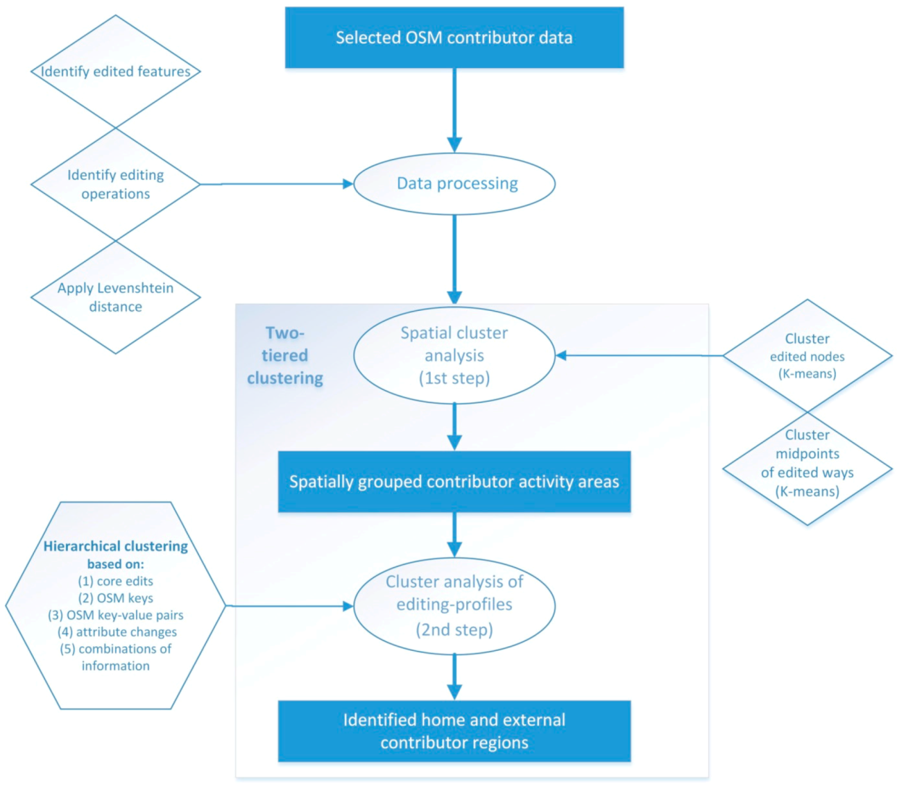
3. Areal Delineation of OSM Contributor Information

3.1. Data Preparation and Contributor Selection

As of August 2014, the OSM project has more than 1.7 million registered members with only a small percentage actively contributing to the dataset on a regular basis [17]. To test the proposed approach for delineating home and external region we chose 13 highly active OSM members, representing an adequate sample size to conduct a qualitative analysis and allowing for the evaluation of the feasibility of the proposed method. Each of the selected members collected information in three or more countries and has been actively contributing to the project for more than 50% of the days since his or her registration to the project. Further, to exclude users with edits originating from bots, automated scripts or imports, we compared the number of created and modified nodes with the number of changesets for each remaining member and excluded those contributors where the number of contributed or changed nodes per changeset exceeded a value of 4000 which seemed unreasonable for manual editing. A changeset stores all data modifications done by one contributor during one session and its extent encompasses all the changes made to the OSM database in that particular session. From this list of 141 users, 13 were randomly chosen, and their contribution data utilized for further analysis. We limited the number of analyzed users to 13 since the focus of this study was to determine the feasibility of the proposed cluster methodology, which required testing various cluster approaches and manual evaluation steps. Thus, this study is meant to be of exploratory nature, and the method, whose initial results are analyzed for the 13 chosen users, could then be automated in the future for a more stringent quantitative analysis. Table 1 summarizes the data collection efforts for the 13 selected contributors which were extracted from the OSM full history dump file dated 2 August 2013.
Table 1. Selected OpenStreetMaps (OSM) contributors with their activity statistics.
OSM MemberCreated NodesModified NodesNo. of ChangesetsNo. of CountriesActive Days (abs.)Active Days (%)
1325,139145,951236912145657%
2429,962146,510381115108482%
3917,417164,61244861383377%
4402,783119,26969158128087%
5333,075101,1097470389656%
6779,798338,74914,81011158686%
7573,13379,0084577472287%
8920,702112,48920,39814182784%
9774,395299,25716,3407140287%
10475,3662,090,48121,1884197988%
11949,472330,92759464129881%
12471,26860,7591137372784%
13340,912200,77122601162585%
After processing the full history dump file, the data was imported into a PostgreSQL database for further analysis as a table that included all features with their versions. Figure 1 shows the workflow of data processing, areal delineation and hierarchical cluster analysis of editing profiles following the selection of 13 active OSM contributors and the import of OSM raw data into the database. A Java tool was used to extract the operations on point or line features for each selected contributor. For this purpose, all adjacent versions of each feature created by any OSM member were compared and evaluated regarding any type of edits between them. The data edits carried out by the contributor of interest were then summarized as a number of operations for each feature. In OSM coding, features (nodes, ways, and relations) are described through tags. Each tag consists of a key and a value and is written as key = value. A key broadly describes an element (e.g., a highway) or attribute associated with an element (e.g., speed limit), and the value more specifically describes its accompanying key. OSM uses a total of 26 suggested primary feature keys, including building, highway, or landuse.
The first set of operations that were considered for area delineation include common editing tasks for nodes and ways, such as adding a primary key-value pair to a point (e.g., amenity = school) or adding a node to a way feature. This set of operations is referred to as core edits from now on. Table 2 lists which operations for nodes and ways were considered for core edits. The first three operations (first line) refer to edits of keys or values on any tag (except for primary key or value or source tag), and the next three operations refer to operations on primary key-value tags only. This is followed by two geometry operations and two way specific operations.
Figure 1. Data analysis flowchart.
Ijgi 03 01211 g001
The data were also specifically examined for operations on feature attributes that would presumably require local knowledge and could not be performed based on information from aerial images. Although some of this information, such as street name and address could be looked up from alternative sources, we believe that the majority of the OSM data contributors are committed to collecting data on their own and providing first-hand information to the OSM project. The feature attributes under consideration are listed in the lower portion of Table 2. Some of these attributes have a corresponding key in the OSM feature documentation, such as name or surface, whereas other attributes in the table consider several OSM tags simultaneously for comparison and detection of a change in attributes. For example, general restrictions for a road (last row in Table 2) include, among others, keys maxheight (maximum height), maxspeed (maximum speed), or maxwidth (maximum width). A change in any of these values would count as an update for this attribute.
Table 2. Operations considered for the identification of home and external region.
OperationsNodeWay
Core editsRemove/add/update tagxx
Remove/add/update primary tagxx
Add geometry (new feature)xx
Change geometry positionx
Remove node from way x
Add node to way x
Attribute changesNamexx
Addressxx
Traffic signsx
Crossingx
Cycleway x
Surface x
Foot x
Oneway x
Restrictions motorized x
General restrictions x
To exclude minor edits on attribute value information from counting, such as changing the capitalization in a street name between two versions of a feature (which would not require local knowledge), only attribute changes were considered where a Levenshtein distance larger than three was detected between both compared string values of an attribute.

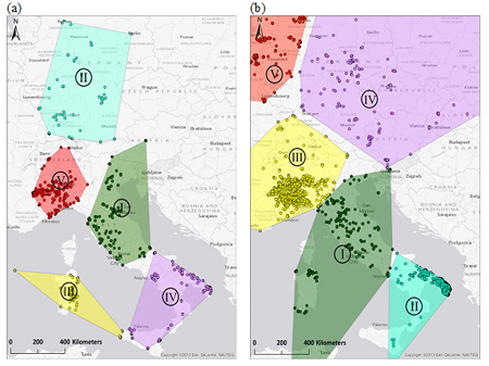
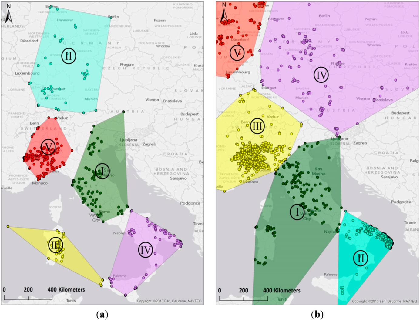
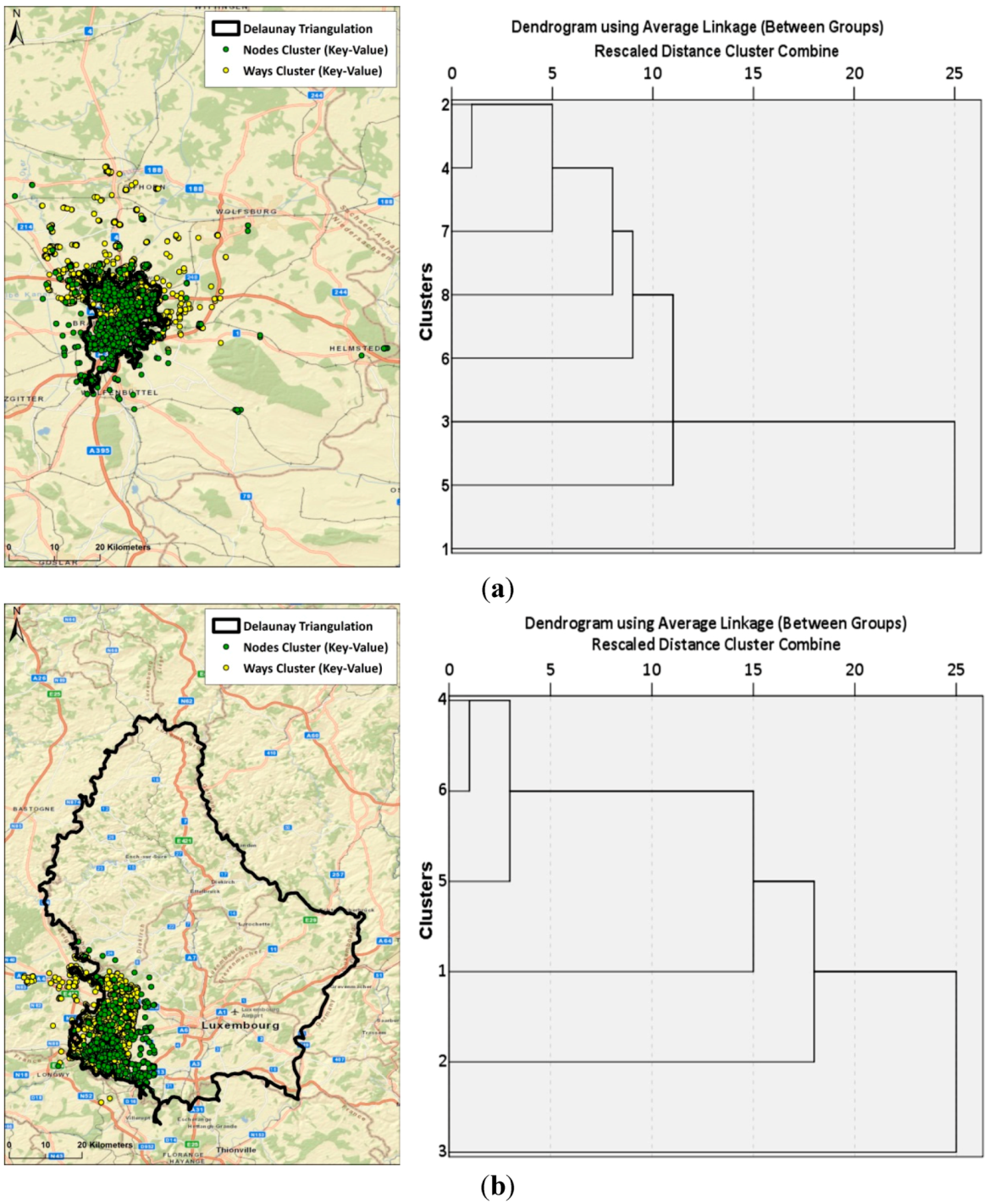
3.2. Clustering Step 1: Spatial Delineation of Activity Areas through k-Means Clustering

The fundamental idea of the proposed areal delineation approach of home and external region is that editing patterns of an individual contributor are different between these regions, where editing patterns can be analyzed separately for node or way features. Edits to a feature can occur along any of the operations listed in Table 2 and be stored for the feature as an n-dimensional vector containing 0 and 1 values, where n is the number of operations under consideration. Similarly, one can also analyze which keys or key-value pairs of edited features are affected by edits. Thus, the n-dimensional vector can be extended by the number of key or key-value categories if they are considered. Such a vector represents then an editing profile for an individual feature.
We expect that clustering of features based on their associated editing profiles will reveal a separation between features located in the home and external region. Although some edits will be primarily found in home regions only, such as adding a speed limit tag to a road, this number of edits will be small compared to all edits being made in any region. Therefore, as some tests revealed with the available dataset, clustering applied at the feature level, e.g., using the TwoStep clustering algorithm [42], did not result in distinct patterns between regions but a cluttered appearance of home and external regions. It is more informative to capture the characteristics of feature edits within pre-defined areas through summarizing the edits on features in these areas (first step), which gives an aggregated editing profile for each area. Next, one can cluster the pre-defined areas based on the similarity between aggregated editing profiles using non-spatial attributes only (second step). Thus, the first step consists of spatially clustering edited nodes (or midpoints of way features, respectively) using Easting and Northing coordinates of features. Although more advanced clustering approaches exist, such as spectral clustering, we used k-means clustering, which makes the proposed method more widely applicable. Also, although k-means clustering limits the detection of clusters to convex shapes [43] this should not be a problem for this type of analysis when choosing k sufficiently large to cover areas of city size or smaller, since home regions, which are typically found in urban areas, can be expected to be of convex shape. That is, even if a data contributor performs daily activities at different locations in a city, e.g., home, work, shopping or leisure, and collects data associated with these locations, the mapped areas can be circumscribed through a convex polygon.
For the data preparation, line geometries for ways were replaced with their midpoints. Further, each feature was mapped only once, even if it had several versions in the history dump file. We tried different k-values (i.e., spatial clusters) for nodes and ways of each of the 13 contributors, and started off with relatively small k-values (in the range of 5–10) that seemed to visually provide a meaningful spatial grouping of nodes. Later on, in combination with step 2 of the clustering approach, we increased k-values to be able to obtain a more spatially refined delineation of the home region. Figure 2 shows the regions generated through k-means clustering on nodes (a) and way midpoints (b) for one of the selected 13 contributors.
Figure 2. Generated k-means clusters for (a) nodes (5 groups) and (b) ways (seven groups—only five shown in the visible extent) for a selected OSM contributor.
Ijgi 03 01211 g002
Summarizing edit counts for each k-means cluster of a user gave k aggregated editing profiles vectors, i.e., one profile for each pre-defined area. Each aggregated profile vector is thus a row with n columns, where n is the number of operations, key, and key-value categories under consideration. The numerical values in a row were computed as the total number of edits for a cluster falling into the editing category under consideration, followed by division by the number of rows of edits in that k-means cluster. This was repeated for all k groups to give a matrix of aggregated profile vectors. Table 3 shows part of such a matrix of node edits for one OSM contributor. In this example, the spatial delineation led to five k-means groups. The value of 0.012, e.g., found in the first row under the “AddTag” column indicates that in k-means cluster #1 1.2 percent of edits included adding a non-primary key tag.
Table 3. Example editing profile for a selected contributor.
K_grpK_grp SizeRem TagAdd TagUpd TagKey Sum1Key Sum2KeyVal Sum1KeyVal Sum2
12450.0000.0120.0000.0000.9920.0000.976
2970.0000.0100.0100.0000.7630.0000.763
3910.0000.0000.0000.0000.9890.0000.989
42310.0000.0130.0000.0000.9610.0000.887
516620.0160.2230.0760.0020.7640.0010.487

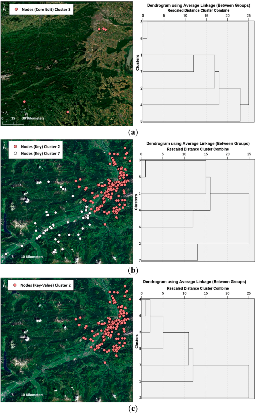
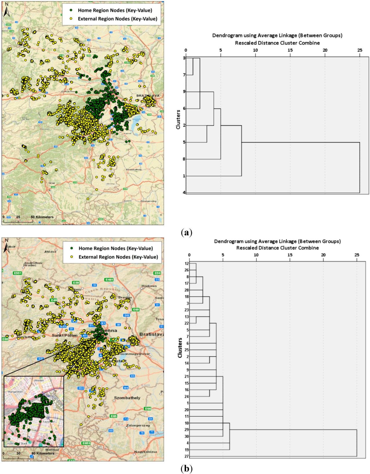
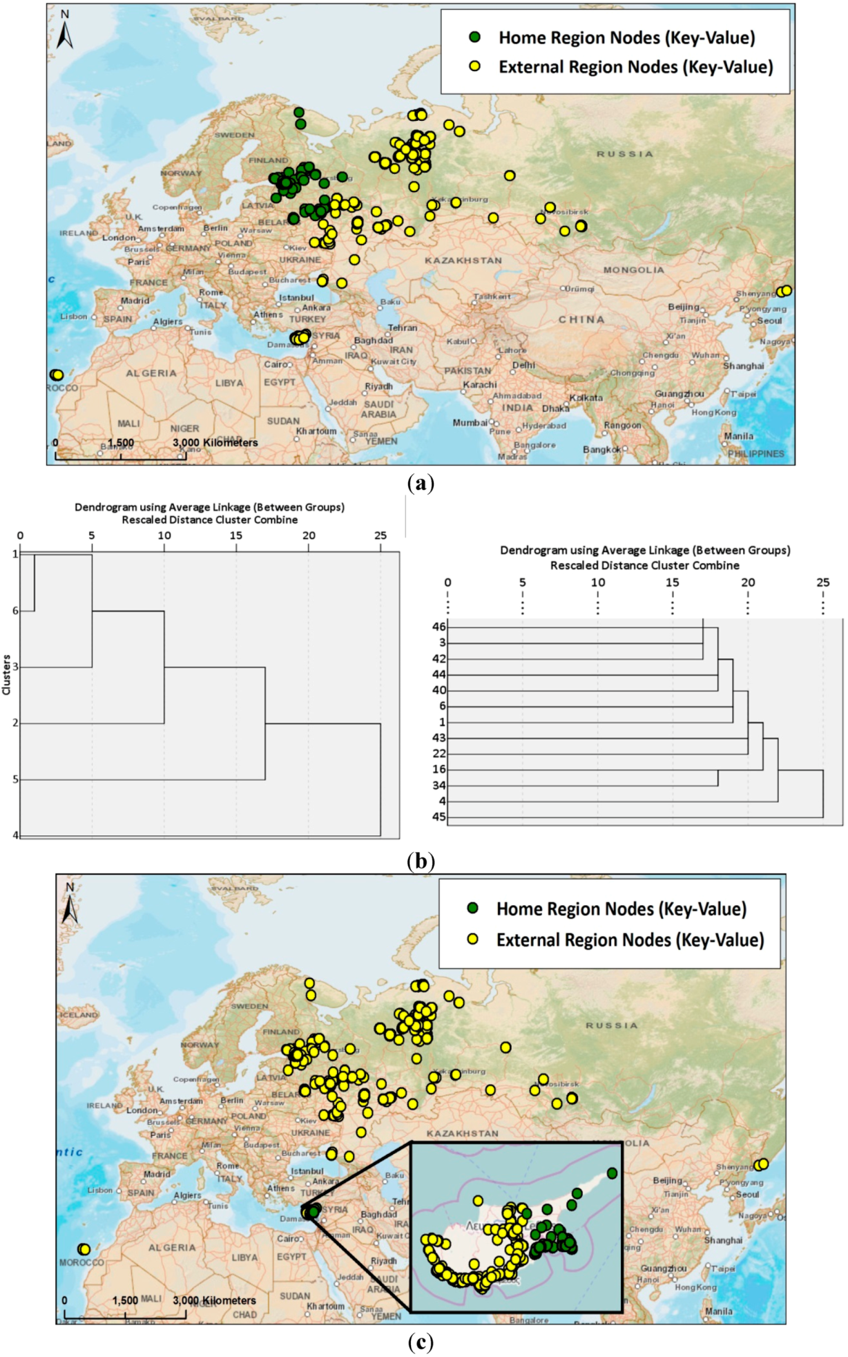
3.3. Clustering Step 2: Identification of Home and External Region through Hierarchical Clustering of Region-Based Editing Profiles

Next, a hierarchical cluster analysis was applied to the k clusters (called cases) with their aggregated editing profiles, where the last two clusters in the agglomeration schedule would be expected to show the home region (ideally consisting of only one case) and the external region (the cluster with the remaining cases). We tested different subsets of operations (see Table 2) and key-value information to be used as information in the aggregated editing profiles in the hierarchical clustering process, which are (1) core edits; (2) keys; (3) key-value pairs; (4) attribute changes; and (5) some combinations of this information. While attribute changes resulted in a cluttered cluster pattern of pre-defined regions with regards to separating home and external region, methods (1) to (3) and their combination provided generally better results, most of which were in-line with those of prior approaches to home area delineation [17]. Several hierarchical clustering methods, such as Ward’s method or Average Linkage between groups were applied, but no effect on the sequence of clustering in the agglomeration schedule was observed.
Figure 3 shows point clusters and dendrograms as a result of the hierarchical clustering process of node edits for one selected contributor, using core edits (a), keys (b) and key-value pairs (c). We considered those cases of the dendrogram as home region that were part of the two final clusters in the agglomeration schedule and within the cluster containing the smaller number of cases. In this example, the core edit information identified two smaller clusters as home regions, which include one somewhat dispersed cluster in eastern Austria (Figure 3a) (cluster #3, 8 points) and one in the US (cluster #6, 1 point). This seemed unlikely to be a home region both based on the spatial distance between the two clusters but also because of the small number of nodes in both clusters. This example demonstrates a limitation of the proposed clustering approach, which is that k-means groups consisting of very small point numbers may have a distinct profile due to a few edits which are then in the hierarchical cluster process identified as home region. Thus, one should keep a minimum number of points in each k-means region before the hierarchical cluster analysis.
Figure 3. Results of hierarchical cluster analysis using core edits (a) (only cluster #3 shown in the visible extent), key (b) and key-value (c) information of edited nodes.
Ijgi 03 01211 g003
Another approach to avoid this problem is to remove spatially isolated points before the cluster analysis, since a home region would consist of more than just a few points.
The key information of edited features helped to delineate two of the pre-defined clusters in the greater Kufstein (Austria) area (Figure 3b) as home region (cluster #2 and #7). Next, using the key-value combination as characteristics in the hierarchical clustering process, the potential home area is narrowed down to just one region, i.e., the close vicinity of Kufstein (cluster #2 in Figure 3c).
Table 4 describes how many cases (i.e., pre-defined k-means areas) are part of the smaller of the two final clusters in the dendrograms (denoting the home region) as a result of hierarchical clustering applied to edits of nodes and way midpoints. A dash (-) indicates that no plausible home region could be identified based on the hierarchical cluster process, which were either disconnected areas or remote areas with only few points. An example that showed both these effects was provided in Figure 3a. If not caused by just a few isolated points, disconnected regions appearing as cases in the final cluster indicate in general that there is no single geographic home region but that the user is travelling and performing similar data edits and contributions in different parts of the mapped regions. Such a situation may, for example, occur if the user relocates after having joined the OSM community, and continues to contribute and edit data. In Table 4, however, disconnected regions found in the core edits and keys columns when marked as a dash, are a result of insufficient information to delineate a primary activity cluster, both for nodes and ways, as opposed to clustering results obtained through consideration of the keys or key-value columns.
Table 4. Number of identified k-means cluster groups in home regions.
OSM MemberCore EditsKeysKey-Values
NodesWaysNodesWaysNodesWays
1--2111
21-1111
31-1212
4----11
5---111
61-1111
7--1111
8----11
9-11-11
101---11
11--1---
12----11
13---111
TOTAL SUCCESS41771211
The results from the 13 tested contributors showed also that core edits of nodes carry more information to distinguish between home and external regions than ways, while this difference could not be observed when using keys or key-values.

4. Evaluation

4.1. Comparison of Cluster Methods

Since providing one’s home region is not required when signing up for an OSM user account, there is no reference dataset available that provides a contributor’s self-defined home region. Therefore, the presented areal delineation approach was evaluated by comparing the extent of the identified home regions with those extracted from a previously introduced method based on a Delaunay triangulation which utilizes the centroids of all changesets created by the contributor under consideration [17].
Figure 4. Results of the two-tiered k-means/hierarchical clustering method and the Delaunay triangulation method for two selected OSM contributors showing a large overlap (a) and clear differences (b) between results from both methods.
Ijgi 03 01211 g004
Additionally, all 13 contributors were contacted individually via the OSM message system which allows OSM members to exchange messages as long as both participants are registered with the project. The contributors were asked to verify or disprove the home region visualized by the “How did you contribute to OpenStreetMap?” website (http://hdyc.neis-one.org/), which utilizes the aforementioned Delaunay triangulation method to determine the home region of a contributor. Seven of the 13 contributors responded to the initially sent message and provided a description of their actual home region.
Figure 4 overlays the delineation results from both methods for two of the selected 13 OSM members. The point clouds indicate features (nodes or way mid-points) in the home area region identified through the hierarchical clustering approach using key-value information. The polygons with black outline indicate the home activity area resulting from the Delaunay triangulation. Figure 4a shows a case where the two methods result in the same general home region (Braunschweig, Germany). The 2-tiered clustering approach covers, however, a larger area due to the larger pre-defined k-means regions. This example demonstrates also a good match between home regions based on node (green) and way (yellow) edits within the 2-tiered clustering approach. The dendrogram to the right is shown for node clusters, and points of cluster #1 are mapped to the left. Figure 4b illustrates how the use of key-value information can help to determine a more refined home area compared to the Delaunay triangulation in some cases. While the triangulation polygon covers an area that is almost identical to that of Luxemburg, the point cloud for nodes indicates a smaller home area of the contributor in the southwestern region of Luxemburg, slightly reaching into Belgium and France. The latter region matched more closely to what the contributor of this region defined as one of his main mapping areas in his response.

4.2. Classification Sensitivity

A perfect spatial overlap between the two-tiered cluster method and the triangulation method cannot be achieved due to the arbitrary choice of k-means cluster regions in the first step, which determines the spatial resolution of the hierarchical clustering step. For example, in Figure 5a the identified home cluster for nodes (green) based on a low k-value of nine covers Vienna (Austria) and its surroundings (cluster #4), whereas Figure 5b with a larger k-value of 30 narrows down the home region to a few city districts (cluster #27), matching the information provided by the contributor during the email exchange more closely.
Whereas both dendrograms in this particular case show a distinct pattern with a single cluster as home region, the choice of the k-means cluster number must balance two conflicting objectives, which are to aim for a high spatial resolution of the home area (i.e., a high k-value), while at the same time obtaining a representative aggregated editing profile for each k-means cluster for successful hierarchical clustering afterwards (i.e., avoid clusters containing only very few points by choosing a reasonably low k-value).
Some OSM contributors do not limit their detailed data collection efforts to a single area, in which case the areal delineation of a single home region proves to be problematic. Figure 6b,c illustrates for OSM member 11 (compare Table 4) how the home region changes when increasing the k-value. Using k = 6, the dendrogram (Figure 6b) suggests that the larger St. Petersburg (Russia) area (cluster #4) represents the home region of the contributor (Figure 6a, green dots). After increasing the k-value to 50 to identify a smaller, more distinct home region, the identified area changes to the eastern part of Cyprus (Figure 6d), corresponding to case #45 in the dendrogram (Figure 6c). The truncated dendrogram shows 13 of the 50 clusters at the end of the agglomeration schedule of which eight are located in the St. Petersburg area and could potentially be merged into one larger home region. However, the last 13 cases also include clusters for Tenerife and Moscow, besides Cyprus, revealing no geographically distinct home area.
Figure 5. Improved delineation of home region through an increase of the k-value from 9 (a) to 30 (b).
Ijgi 03 01211 g005
Figure 6. Delineation of multiple home regions through increase of k-value.
Ijgi 03 01211 g006
The obtained results were confirmed by the contributor, who stated that the delineation of a single home area would be problematic in his particular case. Extensive traveling in recent years and similar detailed mapping efforts in all of the visited regions make the delineation of a single home region difficult. We expect a similar type of cluster results also from contributors who temporarily leave their home country to collect OSM data abroad, e.g., for NGO work or for the Humanitarian OpenStreetMap Team (HOT) [44], where they would then become “de-facto” locals and reveal similar mapping behavior as in their prior home region. The hierarchical clustering analysis would then show different home regions based on the selected k-value, indicating that there is no single home region for that user.
Thus, compared to the purely spatially based Delaunay triangulation method, the integration of editing information in combination with k-means clustering provides some additional means to understand whether an OSM contributor has a single, cohesive home region or an activity region consisting of disconnected parts. More specifically, a variation of k-values and a subsequent review of the resulting dendrogram structure can help to differentiate between both situations. That is, if there is an overlap between areas identified as home regions based on a small but also on a large k value, this is an indication of a single home region. An example is the situation shown in Figure 5, where the home region gets refined through an increased k value of 30 and the refined region is still within the more coarse area originally identified as home region with an initial lower k value of 9. We expect this kind of successive delineation pattern also for users who have a cohesive home region but who contribute in those mapping parties where contributors from abroad focus on agreed upon areas and digitize features from satellite images [45]. The edits conducted in these mapping parties will be of a similar composition as those for other external areas mapped by a user and thus not make users “de-facto” locals.
As opposed to this, disjoint geographic areas of mapping activities with changed k-values, as shown in connection with Figure 6, indicate that there is no single home region. For the same situation, the Delaunay triangulation reports St. Petersburg as a home region, which is only partially true since also other parts should be considered as home regions. This illustrates one of the advantages of the proposed two-tiered clustering approach.

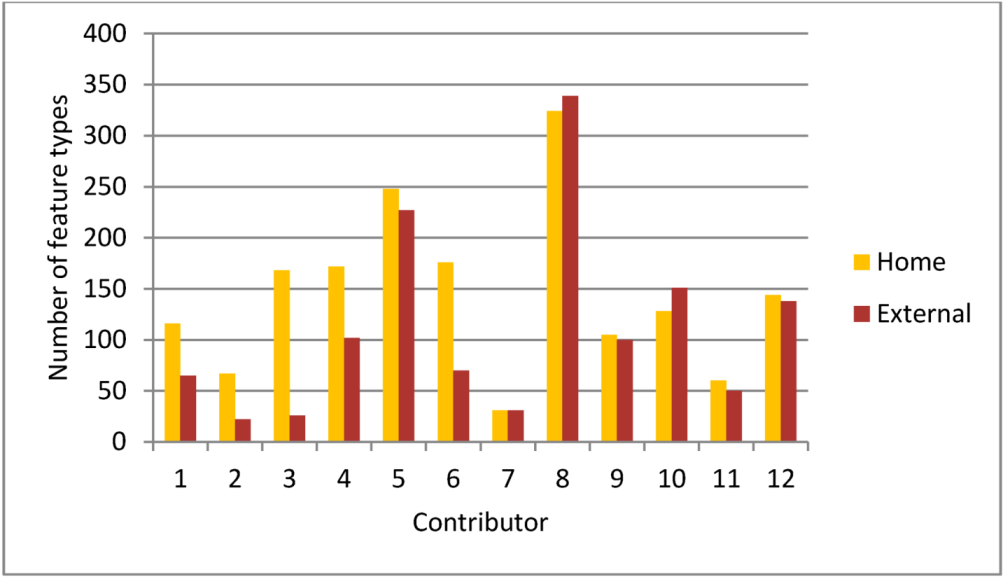
4.3. Diversity and Activity

After the areal delineation of the home and external regions, it was analyzed how many different feature types were edited and on how many days edits were performed in the home and external region for each contributor. A larger diversity of features would imply that the contributor collects more details for a particular area of interest, representing the local knowledge that many VGI enthusiasts consider as one of the main advantages of the OSM project. It needs to be pointed out that feature type diversity is not equally distributed between different geographic regions. More specifically, feature diversity, e.g., measured by variety of amenities, is larger in urban environments than in less populated rural areas. Thus, an OSM contributor exhibiting a larger diversity of mapped features in a home region that is located in an urban environment compared to external regions located exclusively in rural areas would not necessary reflect a higher level detail of data collection effort in the home region, but be a product of the natural distribution of feature diversity. However, each of the selected 13 mappers, since being highly active, contributed data in several distinct densely populated areas. Thus, a larger variety of mapped features in the home region (which comprises typically only one city or city district), indicates in fact a more detailed mapping effort than in external regions, which in our analyzed cases, also include (other) urban areas.
For the 12 successful attempts of areal delineation based on key-value annotations for nodes (compare Table 4), the analysis revealed that among almost all contributors home regions had a larger diversity of features than external regions (Figure 7), although the spatial extent of home regions is smaller than that of external regions. It should be noted that with an increased k-value within the k-means clustering, and thus smaller home region compared to external regions, it can be expected that the feature diversity decreases for the home region. Thus, the results in Figure 7 are closely tied to k-values chosen for the different mappers in this analysis. The smaller feature diversity in external regions can probably be attributed to the mapping method, i.e., digitizing of roads, buildings, or landuse information from satellite images, which is mostly utilized for remote areas or areas unknown to the contributor. A Wilcoxon matched-pairs signed rank test confirmed that the number of feature types mapped in the home regions is significantly higher than that mapped in external regions (z = −2.045, p = 0.019, 1-tailed). Despite the statistically larger feature diversity in the home regions than in the externals region among analyzed datasets, results for the right-most five contributors give a less clear picture. The similar diversity rates between home and external regions can be explained by the fact that for these contributors the identified home regions were located within urban environments, where external regions in the vicinity provide similar features to be mapped. This suggests that the provided cluster method is unreliable in identifying crisp boundaries of home regions that are located inside an urban environment where the transition between a home and external regions may be gradual.
Figure 7. Diversity of mapping efforts in home and external regions.
Ijgi 03 01211 g007
Similar to feature diversity, we assume that the area with the largest number of days dedicated to mapping activities identifies a contributor’s main area of interest on a temporal level. For the temporal analysis of mapping efforts a similar pattern could be observed (Figure 8). With the exception of two contributors, all OSM members dedicated more days to mapping features in their home region than in the external region. A Wilcoxon matched-pairs signed rank test confirmed that the number of days with mapping activities were significantly higher in the home regions than in external regions (z = −1.961, p = 0.025, 1-tailed). The two contributors that did not follow this trend showed a significantly higher value for mapping days in the external region due to the close proximity of home and external regions, for instance downtown Vienna (home region) and Vienna suburbs (external region).
Figure 8. Temporal spectrum of mapping efforts in home and external regions.
Ijgi 03 01211 g008
The analysis provided in connection with Figure 7 and Figure 8 illustrates why determining the home region of OSM contributors is important: It is an indication of improved data quality in a region through increased activity (number of mapping days) and larger diversity of feature edits conducted by an individual data contributor. Data quality depends, of course, also on the number of different data contributors that share the same home region. A higher number of contributors home to the same region can be expected to lead to even better data quality than this would be the case with only one contributor. This has not been tested in the current study but can be considered as part of future work.

5. Summary and Conclusions

OSM contributor patterns can vary significantly between mapped regions of a contributor. The two-tiered clustering method proposed in this paper utilizes editing information of OSM objects to delineate the home and external region of a contributor. It provides an alternative to existing delineation methods that identify a home region solely based on positional information of feature edits, and provides some additional insight into the distinction between single clusters versus dispersed home regions.
The analysis of node feature diversity in home and external regions revealed that most contributors edited a larger variety of features in home regions than in external regions. This pattern supports the local knowledge connotation that many claim as one of the main advantages of VGI projects, such as OSM. Local knowledge can be obtained from being on-site, allowing for more detailed data collection efforts than mapping from satellite imagery. Similarly the temporal analysis, focusing on the number of days a contributor dedicated to mapping efforts in each region, showed a larger value for home regions than external regions for almost all contributors.
In this study, the proposed two-tiered cluster analysis was conducted manually on a small set of active users to assess its potential, strengths, and weaknesses. The sample size of 13 analyzed users is clearly too small for a quantitative evaluation of the proposed two-tiered cluster analysis, or a qualitative comparison between both discussed cluster methods. Thus, a future task is to automate the two-tiered clustering process to make it applicable to a larger user data set, similar to the Delaunay triangulation approach used in [17]. This would also require the automated distinction between a single cluster vs. dispersed home region, which in the presented study was done by manual exploration of dendrograms and maps by variation of k in the k-means cluster step. For future work, one could consider spatio-temporal cluster approaches instead of k-means clustering to identify mapping regions that different spatially and temporally, and could then be used for hierarchical clustering. Additionally, the potential relocation of a mapper and the corresponding shift of the home region could be investigated in more detail in the near future.
For the 13 analyzed users, the comparison between the results of the proposed two-tiered clustering method and a previously introduced Delaunay triangulation approach showed generally a good match between identified home areas. While the triangulation method solely uses geometries as a source, the clustering method allows for more in-depth analysis due to the additional information considered, such as the edit type or key-value annotations. In cases where the k-means home clusters are too coarse, it was demonstrated that an increased k-value can help refine the identification of the home region. However, the detection of home regions still proved to be problematic for contributors with disjoint mapping area in which detailed mapping efforts took place, such as during holidays or other activities. The proposed two-tiered method works well for active mappers where numerous edits in the spatially delineated areas generate distinct aggregated editing profiles. As opposed to this, too few edits, or too high k-values, respectively, can lead to distinct editing profiles by chance, thus not reflecting a contributor’s true home region. However, a remaining research goal for the future is to assess whether the proposed method works also for less active mappers. Based on the tested examples, a choice of a k-value that results in k-means cluster sizes covering approximately a city or some city districts seems to provide meaningful results, thus avoiding the problem of very small point numbers in the profile clustering. One can also compare cluster results from both methods, e.g., the Delaunay triangulation and the proposed two-tiered cluster method, to gain confidence in the detection of the home region. Both methods help to delineate home from external contributor areas, which creates the foundation for future research that focuses on the interrelation between contributor behavior and quality assessment.

Author Contributions

Dennis Zielstra, Hartwig Hochmair and Pascal Neis conceived and designed the experiments. Dennis Zielstra performed the experiments and analyzed the data in collaboration with Hartwig Hochmair. Francesco Tonini contributed reagents and advice for statistical analysis. Dennis Zielstra wrote the paper with contributions by Hartwig Hochmair.

Conflicts of Interest

The authors declare no conflict of interest.

References

  1. Goodchild, M.F. Citizens as voluntary sensors: Spatial data infrastructure in the World of Web 2.0. Int. J. Spat. Data Infrastruct. Res. (IJSDIR) 2007, 2, 24–32. [Google Scholar]
  2. Girardin, F.; Blat, J.; Calabrese, F.; Fiore, F.D.; Ratti, C. Digital footprinting: Uncovering tourists with user-generated content. Pervasive Comput. 2008, 7, 36–43. [Google Scholar] [CrossRef]
  3. Andrienko, G.; Andrienko, N.; Bak, P.; Kisilevich, S.; Keim, D. Analysis of community-contributed space- and time-referenced data (example of flickr and panoramio photos). In Proceedings of the IEEE Symposium on Visual Analytics Science and Technology, Atlantic City, NJ, USA, 12–13 October 2009; pp. 213–214.
  4. Chen, L.; Roy, A. Event detection from flickr data through wavelet-based spatial analysis. In Proceedings of the 18th ACM Conference on Information and Knowledge Management, Hong Kong, China, 2–6 November 2009; ACM: New York, NY, USA; pp. 523–532.
  5. Schlieder, C.; Matyas, C. Photographing a city: An analysis of place concepts based on spatial choices. Spat. Cogn. Comput. 2009, 9, 212–228. [Google Scholar]
  6. Hollenstein, L.; Purves, R.S. Exploring place through user-generated content: Using flickr to describe city cores. J. Spat. Inf. Sci. 2010, 1, 21–48. [Google Scholar]
  7. Andrienko, G.; Andrienko, N.; Bosch, H.; Ertl, T.; Fuchs, G.; Jankowski, P.; Thom, D. Thematics patterns in georeferenced tweets through space-time visual analytics. Comput. Sci. Eng. 2013, 15, 72–82. [Google Scholar] [CrossRef]
  8. Krumm, J.; Caruana, R.; Counts, S. Learning likely locations. In User Modeling, Adaption, and Personalization; Carberry, S., Weibelzahl, S., Micarelli, A., Semeraro, G., Eds.; Springer: Berlin, Germany; pp. 64–76.
  9. Li, Y.; Shan, J. Understanding the spatio-temporal pattern of tweets. Photogramm. Eng. Remote Sens. 2013, 79, 769–773. [Google Scholar] [CrossRef]
  10. Collins, C.; Hasan, S.; Ukkusuri, S.V. A novel transit rider satisfaction metric: Rider sentiments measured from online social media data. J. Public Transp. 2013, 16, 21–45. [Google Scholar]
  11. Mitchell, L.; Frank, M.R.; Harris, K.D.; Dodds, P.S.; Danforth, C.M. The geography of happiness: Connecting twitter sentiment and expression, demographics, and objective characteristics of place. PLoS One 2013, 8, e64417. [Google Scholar] [CrossRef] [PubMed]
  12. Noulas, A.; Scellato, S.; Mascolo, C.; Pontil, M. An empirical study of geographic user activity patterns in foursquare. In Proceedings of the 5th International AAAI Conference on Weblogs and Social Media, Menlo Park, CA, USA, 19–21 July 2011; Adamic, L., Baeza-Yates, R., Counts, S., Eds.; The AAAI Press: Palo Alto, CA, USA; pp. 570–573.
  13. Mooney, P.; Corcoran, P. Characteristics of heavily edited objects in OpenStreetMap. Future Internet 2012, 4, 285–305. [Google Scholar] [CrossRef]
  14. Arsanjani, J.J.; Barron, C.; Bakillah, M.; Helbich, M. Assessing the quality of OpenStreetMap contributors together with their contributions. In Proceedings of the AGILE 2013, Leuven, Belgium, 5–9 August 2013.
  15. Haklay, M.; Basiouka, S.; Antoniou, V.; Ather, A. How many volunteers does it take to map an area well? The validity of Linus’ law to volunteered geographic information. Cartogr. J. 2010, 47, 315–322. [Google Scholar] [CrossRef]
  16. Neis, P.; Zielstra, D.; Zipf, A. Comparison of volunteered geographic information data contributions and community development for selected world regions. Future Internet 2013, 5, 282–300. [Google Scholar] [CrossRef]
  17. Neis, P.; Zipf, A. Analyzing the contributor activity of a volunteered geographic information Project—The case of OpenStreetMap. ISPRS Int. J. Geo. Inf. 2012, 1, 146–165. [Google Scholar] [CrossRef]
  18. Heipke, C. Crowdsourcing geospatial data. ISPRS J. Photogramm. Remote Sens. 2010, 65, 550–557. [Google Scholar] [CrossRef]
  19. Mooney, P.; Corcoran, P. Analysis of interaction and co-editing patterns amongst OpenStreetMap contributors. Trans. GIS 2013, 18, 633–659. [Google Scholar] [CrossRef]
  20. Gröchenig, S.; Brunauer, R.; Rehrl, K. Estimating completeness of VGI datasets by analyzing community activity over time periods. In Connecting a Digital Europe through Location and Place; Huerta, J., Schade, S., Granell, C., Eds.; Springer: Berlin, Germany, 2014; pp. 3–18. [Google Scholar]
  21. Rehrl, K.; Gröchenig, S.; Hochmair, H.H.; Leitinger, S.; Steinmann, R.; Wagner, A. A conceptual model for analyzing contribution patterns in the context of VGI. In Progress in Location Based Services; Krisp, J.M., Ed.; Springer: Berlin, Germany, 2013; pp. 373–388. [Google Scholar]
  22. Gröchenig, S. Using Spatial and Temporal Editing Patterns for Evaluation of Open Street Map Data. MSc Thesis, Carinthia University of Applied Sciences, Villach, Carinthia, Austria, 2012. [Google Scholar]
  23. Steinmann, R.; Brunauer, R.; Gröchenig, S.; Rehrl, K. Wie aktiv sind freiwillige Mapper? Ein Vergleich der OpenStreetMap-Aktivitäten in den Jahren 2005–2012 am Beispiel der DACH-Region. In Angewandte Geoinformatik; Strobl, J., Blaschke, T., Griesebner, G., Zagel, B., Eds.; Wichmann: Berlin, Germany, 2013; pp. 173–182. [Google Scholar]
  24. Steinmann, R.; Gröchenig, S.; Rehrl, K.; Brunauer, R. Contribution profiles of voluntary mappers in OpenStreetMap. In Proceedings of Action and Interaction in Volunteered Geographic Information (ACTIVITY) Workshop at AGILE 2013, Leuven, Belgium, 14 May 2013.
  25. Haklay, M. How good is Volunteered Geographical Information? A comparative study of OpenStreetMap and Ordnance Survey datasets. Environ. Plan. B Plan. Des. 2010, 37, 682–703. [Google Scholar]
  26. Zielstra, D.; Zipf, A. OpenStreetMap data quality research in Germany. In Proceedings of the 6th International Conference on Geographic Information Science (GIScience), Zurich, Switzerland, 14–17 September 2010.
  27. Neis, P.; Zielstra, D.; Zipf, A. The street network evolution of crowdsourced maps: OpenStreetMap in Germany 2007–2011. Future Internet 2012, 4, 1–21. [Google Scholar]
  28. Zielstra, D.; Hochmair, H.H. Using free and proprietary data to compare shortest-path lengths for effective pedestrian routing in street networks. Transp. Res. Record 2012, 2299, 41–47. [Google Scholar] [CrossRef]
  29. Zielstra, D.; Hochmair, H.H. A comparative study of pedestrian accessibility to transit stations using free and proprietary network data. Transp. Res. Record 2011, 2217, 145–152. [Google Scholar] [CrossRef]
  30. Hochmair, H.H.; Zielstra, D.; Neis, P. Assessing the completeness of bicycle trail and designated lane features in OpenStreetMap for the United States. Trans. GIS 2014, in press. [Google Scholar]
  31. Zook, M.A.; Graham, M.; Shelton, T.; Gorman, S. Volunteered geographic information and crowdsourcing disaster relief: A case study of the Haitian earthquake. World Med. Health Policy 2010, 2, 7–33. [Google Scholar] [CrossRef]
  32. Parker, C.J.; May, A.J.; Mitchell, V. The role of VGI and PGI in supporting outdoor activities. Appl. Ergon. 2012, 44, 886–894. [Google Scholar] [CrossRef] [PubMed] [Green Version]
  33. Parker, C.J.; May, A.J.; Mitchell, V. User centred design of neogeography: The impact of volunteered geographic information on trust of online map “mashups”. Ergonomics 2014, 57, 987–997. [Google Scholar] [CrossRef] [PubMed]
  34. Parker, C.J.; May, A.J.; Mitchell, V. Understanding design with VGI using an information relevance framework. Trans. GIS 2012, 16, 545–560. [Google Scholar] [CrossRef]
  35. Girres, J.F.; Touya, G. Quality assessment of the French OpenStreetMap dataset. Trans. GIS 2010, 14, 435–459. [Google Scholar] [CrossRef]
  36. Mooney, P.; Corcoran, P. The annotation process in OpenStreetMap. Trans. GIS 2012, 16, 561–579. [Google Scholar] [CrossRef]
  37. Keßler, C.; de Groot, R. Trust as a Proxy Measure for the quality of volunteered geographic information in the case of OpenStreetMap. In Geographic Information Science at the Heart of Europe; Vandenbroucke, D., Bucher, B., Crompvoets, J., Eds.; Springer: Heidelberg, Germany, 2013; pp. 21–37. [Google Scholar]
  38. Keßler, C.; Trame, J.; Kauppinen, T. Provenance and trust in volunteered geographic information: The case of OpenStreetMap. In Proceedings of the Conference on Spatial Information Theory: COSIT’11, Belfast, ME, USA, 12–16 September 2011; pp. 1–3.
  39. Zielstra, D.; Hochmair, H.H.; Neis, P. Assessing the effect of data imports on the completeness of OpenStreetMap—A United States case study. Trans. GIS 2013, 17, 315–334. [Google Scholar] [CrossRef]
  40. Hochmair, H.H.; Zielstra, D. Development and completeness of points of interest in free and proprietary data sets: A Florida case study. In Proceedings of GI_Forum 2013, Creating the GISociety, Salzburg, Austria, 2–5 July 2013; Jekel, T., Car, A., Strobl, J., Griesebner, G., Eds.; Wichmann: Berlin, Germany; pp. 39–48.
  41. Perkins, C.; Dodge, M. The potential of user-generated cartography: A case study of the OpenStreetMap project and Mapchester mapping party. North West Geogr. 2008, 8, 19–32. [Google Scholar]
  42. Bacher, J.; Wenzig, K.; Vogler, M. Twostep Cluster: A First Evaluation. 2004. Available online: http://www.opus.ub.uni-erlangen.de/opus/volltexte/2004/81/pdf/a_04-02.pdf (accessed on 16 August 2014).
  43. Abubaker, M.; Ashour, W. Efficient data clustering algorithms: Improvements over Kmeans. Int. J. Intell. Syst. Appl. 2013, 5, 37–49. [Google Scholar]
  44. Humanitarian OpenStreetMap Team [HOT]. Available online: http://hot.openstreetmap.org/projects (accessed on 16 August 2014).
  45. OpenStreetMap Operation Cowboy. Available online: http://wiki.openstreetmap.org/wiki/Operation_Cowboy (accessed on 16 August 2014).

