Article

Improving Inland Water Quality Monitoring through Remote Sensing Techniques

by
Igor Ogashawara
1,2,* and
Max J. Moreno-Madriñán
3
1
Remote Sensing Division, National Institute for Space Research (INPE), Avenida dos Astronautas, 1758, São José dos Campos 12227-010, Brazil
2
Department of Earth Sciences, Indiana University-Purdue University Indianapolis, 723 W. Michigan Street, SL118, Indianapolis, IN 46202, USA
3
Department of Environmental Health, Fairbanks School of Public Health, Indiana University, 714 N. Senate Avenue, EF 206, Indianapolis, IN 46202, USA
*
Author to whom correspondence should be addressed.
ISPRS Int. J. Geo-Inf. 2014, 3(4), 1234-1255; https://0-doi-org.brum.beds.ac.uk/10.3390/ijgi3041234
Submission received: 9 June 2014 / Revised: 13 October 2014 / Accepted: 30 October 2014 / Published: 14 November 2014
(This article belongs to the Special Issue Remote Sensing and Geospatial Technologies in Public Health)

Abstract

:
Chlorophyll-a (chl-a) levels in lake water could indicate the presence of cyanobacteria, which can be a concern for public health due to their potential to produce toxins. Monitoring of chl-a has been an important practice in aquatic systems, especially in those used for human services, as they imply an increased risk of exposure. Remote sensing technology is being increasingly used to monitor water quality, although its application in cases of small urban lakes is limited by the spatial resolution of the sensors. Lake Thonotosassa, FL, USA, a 3.45-km2 suburban lake with several uses for the local population, is being monitored monthly by traditional methods. We developed an empirical bio-optical algorithm for the Moderate Resolution Imaging Spectroradiometer (MODIS) daily surface reflectance product to monitor daily chl-a. We applied the same algorithm to four different periods of the year using 11 years of water quality data. Normalized root mean squared errors were lower during the first (0.27) and second (0.34) trimester and increased during the third (0.54) and fourth (1.85) trimesters of the year. Overall results showed that Earth-observing technologies and, particularly, MODIS products can also be applied to improve environmental health management through water quality monitoring of small lakes.

1. Introduction

Besides traditional multiple uses of inland waters by mankind, urban lakes also provide services, such as storm-water buffer, waste removal and recreation [1]. Because of such multiple uses and services, the deterioration of water quality in urban lakes has been a serious ecological and social problem that can severely affect human health [2]. Indeed, the public health implications of surface water quality are among the main concerns related to aquatic systems. In inland waters in general, one of the greatest problems is the eutrophication process caused by the increase of nutrient inputs. This process has been affecting the ecological health of many shallow lakes worldwide [3], and urban lakes are not an exception in this category. This condition is enhanced by the increasing shortage of available water resources, growing urbanization and the lack of a water governance system, which affects mainly recently urbanized countries. These and other human-related factors, along with climate variations and rising temperatures, have been suggested as possible factors triggering an increasing trend in cyanobacteria abundance [4]. Among the problems caused by eutrophication, special interest is placed on the toxins and taste and odor production by some species of algae and cyanobacteria. Such toxins can enter the body via oral, dermal and inhalation routes through drinking water, freshwater food consumption and recreational water activities. Moreover, they can poison or even kill humans and animals that consume contaminated water and food [2,3]. Although low concentrations of toxins from cyanobacteria and algae may be adequately removed from the source water by conventional water treatment, the same may not be the case with high initial concentrations [5]. In Florida, an increased risk for liver cancer has been associated with residence within the area served by a surface water treatment plant as compared with residents living in contiguous areas [6].
The first scientific report of animal contamination from a harmful algal bloom (HAB) related to cyanobacteria occurred in 1878 by George Francis [7]. He reported a HAB in Lake Alexandrina (Australia) and observed that after animals drank its water, they were poisoned and rapidly died. The author even observed the time that cyanotoxins took to cause death in different animals: in sheep, from six to eight hours; in horses, from eight to twenty-four hours; in dogs, from four to five hours, and in pigs, from three to four hours. One of the first reported cases of human casualty associated with cyanobacteria and their toxins came about in 1996, in the city of Caruaru, PE, Brazil, where exposure through kidney dialysis led to the death of approximately fifty patients [8]. This disaster raised the awareness of water quality managers, environmental agencies, policy makers and the general public to the problem of HABs. Likewise, this incident warned about the need for a reliable and constant monitoring of HABs by environmental and public health programs. The World Health Organization’s (WHO) Working Group on the Protection and Control of Drinking Water Quality identified cyanotoxins as an issue requiring urgent attention. In the United States, 22 hospitalizations out of two hundred and ninety-six cases were reported by the Center for Disease Control and Prevention (CDC) during the years 2009–2010 [9].
Phytoplankton primary production has been regarded as a reliable and accurate indicator to monitor eutrophication and HABs [3]. In turn, several research studies have confirmed that chlorophyll-a (chl-a) is a universally acknowledged indicator of phytoplankton abundance and trophic state due to its visible manifestation and for being part of the eutrophication process [10,11]. Thus, chl-a concentration has been long applied as an indicator for water quality monitoring of inland waters. Although chl-a is relatively easily measured in comparison to algal biomass, traditional methods consist of field water sampling and laboratory analysis, which are usually costly and time consuming [12]. Consequently, water quality monitoring is not conducted with enough regularity, which, in turn, may lead to limitations in the study of the environmental dynamics.
Because of these facts, there is rapidly growing interest in the application of satellite remote sensing technology in environmental management. The reasons for such interest are based on several advantages, such as: (1) the synoptic view of the satellite images, which allows the user to retrieve information from large geographic areas; (2) the acquisition of data from places that are otherwise difficult to access; (3) the temporal resolution, which can provide a historical dataset allowing the users to retrieve information from the past [13]. Consequently, remote sensing technology has been increasingly used to facilitate the decision-making process of environmental managers and policy makers.
Numerous studies have focused on deriving chl-a concentration information from remote sensing satellites in inland water bodies [11,12,14,15]. However, there are several limitations related mainly to the sensor resolutions required to monitor aquatic systems with such high spatial irregularities and often small areas. Ogashawara et al. [14] addressed the problem of spatial, temporal and spectral resolutions of satellite images in the monitoring of inland waters. Regarding spatial resolutions, the authors studied a small water body in which the use of a sensor with low spatial resolution caused high interference in the signal from adjacent (not targeted) features. The authors also discussed the importance of spectral resolution, since for turbid inland waters, the bio-optical models are usually based on the optical properties located at the red and near-infrared (NIR) regions of the spectrum [16,17,18]. These algorithms used the ratio of the chl-a reflectance peak around 700 nm (NIR) to the reflectance near 675 nm, which is the red chl-a absorption band [19,20]. The temporal resolution is also a very important aspect of remote sensing estimation of chl-a in aquatic systems, because of the quick responses of chl-a to changes in the environment; thus, a good temporal resolution is crucial for consistent water quality monitoring.
The objective of this study was to assess the applicability of the Moderate Resolution Imaging Spectroradiometer (MODIS) daily product of surface reflectance (MOD09GA) to detect chl-a concentration in a small inland lake, using as a case Lake Thonotosassa, a suburban lake in Tampa, FL, USA, which has experienced episodic blooms of blue-green algae (cyanobacteria) [21]. We justify the use of the MOD09GA by its spatial resolution (500 m), which is higher than the spatial resolution of the spectral bands usually used in ocean color algorithms. Moreover, since this is a daily product, it could improve the temporal monitoring coverage for algal blooms in this aquatic system, which currently occurs on a monthly basis for three sampling stations by traditional methods. Besides ecological concerns for this lake’s water quality, there are public health concerns related to its designated use for human recreation and the fact that the outflow of this lake discharges into the Hillsborough River and, ultimately, into the water reservoir that provides the drinking water supply to the City of Tampa.
The specific goals of this study were: (1) to evaluate the use of the most common ocean color algorithms applied on MODIS Level 0 products for the estimation of chl-a estimations; (2) to evaluate the use of 1-km spatial resolution MODIS spectral bands in the retrieval of chl-a; and (3) to propose an empirical algorithm for chl-a concentration estimation in Lake Thonotosassa with seasonal calibrations using the MOD09GA product. These goals were motivated by our intention to propose a more consistent monitoring of chl-a (both temporally and spatially) for public health management in this lake, further developing a methodology that could be applied to generate the appropriate algorithms to be used in similar lakes in other areas.

2. Materials and Methods

2.1. Study Site

The study site for this research is Lake Thonotosassa (28°03′N, 82°16′W), which is located in a suburban area in Hillsborough County, Florida, USA (Figure 1). The lake is supplied mainly by the runoff from surrounding citrus groves and from Baker Creek, an improved drainage canal originating in Dover, Florida [22]. The lake has a surface area of 3.45 km2, with a mean depth of 3.5 m and a maximum depth of 5.1 m. The water temperature in Lake Thonotosassa varies from 14 to 34 °C during the year, with a mean of approximately 25 °C. Short-term thermal stratification (less than 5 °C from the surface to bottom) and hypolimnetic oxygen deficits occur in the deeper parts of the lake during the warmer months (May–October) [23]. Cowell et al. [22] showed that the lake was in advanced stages of eutrophy by analyzing its limnological characteristics. The authors observed that the eutrophication process occurred because of 15 years of artificial enrichment by organic wastes from domestic sewage and citrus processing plants. Their findings showed that inorganic nutrient levels were high, as well as oxygen deficits in the hypolimnion and at the mud-water interface. The phytoplankton community was large and dominated by cyanobacteria that generate a primary productivity rate comparable to those of grossly polluted lakes.
The high eutrophication levels in Lake Thonotosassa got the attention of policy makers, and consequently, the Environmental Protection Commission of Hillsborough County (EPCHC) has monitored its water quality since 1975. According to the Southwest Florida Water Management District (SFWMD) [21], the annual averages for total phosphorous concentrations for Lake Thonotosassa for the period of 1992–2000 varied from 0.3 to 0.77 mg/L. Average annual total nitrogen for the same period ranged from 1.8 to 4.1 mg/L. These high concentrations of nutrients led to high algal biomass (chl-a concentrations), which has ranged from 62 μg/L to 179 μg/L during the same period. Under current state standards, average chl-a levels greater than 20 μg/L are considered indicative of poor water quality for aquatic life in Florida lakes [24].

2.2. Dataset

2.2.1. Limnological Dataset

The water quality data from Lake Thonotosassa used in this study were collected and provided by the EPCHC. Data were collected monthly as part of routine water quality monitoring programs from three sampling stations, one located at the inlet, another at the middle and a third one at the outlet regions of the lake (see Figure 1 for the locations). Such a monitoring program also covers Tampa Bay and water bodies in its watershed. In this study, we used measurements of total phosphorus (TP), total nitrogen (TN) and chl-a concentration, which were collected during the time period between 2001 and 2011. Monthly water samples were analyzed by the EPCHC laboratory, which is a National Environmental Laboratory Accreditation Program (NELAP) certified laboratory. Water quality analyses were conducted using a combination of Environmental Protection Agency (EPA) and American Public Health Association (APHA) standard methods, following quality assurance and quality control (QA/QC) guidelines from both methodologies and all NELAP QA/QC rules. The TP concentration was determined following the EPA 365.4 methodology; the TN concentration were calculated by the sum of the total Kjeldahl nitrogen (TKN) and nitrate/nitrite nitrogen, where TKN was determined by EPA 351.2 and the nitrate/nitrite nitrogen concentration by Standard Methods 4500 NO3 F (SM 4500 NO3 F) [25]. The Chl-a concentration was determined by Standard Methods10200 H (SM 10200 H) [25], using acetone and a tissue grinder. More details on the methods of the laboratory analysis and sampling of in situ data have been described previously [18,26,27].
Figure 1. Location of Lake Thonotosassa in the State of Florida, USA, and the location of sampling points from the Environmental Protection Commission of Hillsborough County.
Ijgi 03 01234 g001

2.2.2. Remote Sensing Products

The remote sensing dataset consisted of two MODIS products. The following MODIS data were used: Level 0 MODIS data (L0_LAC) at a 1-km spatial resolution and Surface Reflectance Daily L2G at a 500-m spatial resolution (MOD09GA). MODIS L0 data were provided by NASA’s Ocean Color Products through their web portal [28]. MOD09GA data were provided by NASA’s Earth Observing System Data and Information System (NASA/EOSDIS) through the Reverb web [29] portal. To process the L0 MODIS products to Level 3 products, we used the SeaWiFS Data Analysis System (SeaDAS) [30]. The MODIS Reprojection Tool (MRT) was used to re-project the MOD09GA dataset to the UTM coordinate system with the WGS-84 datum as the reference. The reflectance values were calculated using the scale factor of MOD09GA for the MOD09GA Collection 5 products acquired on the same day of the limnological collection from 2000 to 2011.

2.3. Ocean Color Algorithms Evaluation

Ocean color algorithms for MODIS usually use the spectral bands with 1-km spatial resolution. As is widely known, such a resolution is not useful for retrieving information from small inland aquatic systems, due to the mixing signal from other targets being different from the intended water body. Nevertheless, we used them for the purpose of comparison with our proposed algorithm. We evaluated three ocean color algorithms implemented in SeaDAS to show how MODIS 1-km bands could not retrieve geochemical data from Lake Thonotosassa.

2.3.1. Algorithms Used for Evaluation

We evaluated three existent chl-a algorithms, which are freely available from SeaDAS: the ocean color 3-band ratio (OC3M) [31], the Garver-Siegel-Maritorena model (GSM) [32] and the generalized inherent optical property (GIOP) [33]. OC3M is a fourth-order band ratio algorithm of remote sensing reflectance (Rrs), which can use two different band ratios: Rrs443/Rrs547 or Rrs448/Rrs547 [31]. The GSM is an optimized semi-analytical algorithm that simultaneously retrieves inherent optical properties (IOPs) from spectral measurements of normalized water leaving spectral radiance (nLw(λ)) [32]. The GIOP model uses the spectral behaviors of several optically-active constituents (OACs) in the water column to apply in an inversion process. This process is based on finding the optimum set of eigenvalues between the modelled Rrs and MODIS Rrs using the Levenberg-Marquardt optimization scheme [33]. These three algorithms are presented and described in Table 1.
Table 1. Functional form of MODIS chl-a algorithms. OC3M, ocean color 3-band ratio; GSM, Garver-Siegel-Maritorena; GIOP, generalized inherent optical property.
AlgorithmReferenceFunctional Form
OC3M[31] c h l a = 10 ( a 1 + a 2 R + a 3 R 2 + a 4 R 3 + a 5 R 4 )
GSM[32] a p h y ,   i = c h l a · a p h y *
GIOP[33] c h l a = a p h y ,   i i a p h y *
From the table, R is the chosen band ratio; a1, a2, a3, a4 and a5 are coefficients from the polynomial equation with the following values: 0.2424, −2.7423, 1.8017, 0.0015 and −1.2280, respectively; aphy,i is the absorption coefficient of phytoplankton, which is substituted in the GSM model for the functional form; aphy,ii is the absorption coefficient of phytoplankton derived from the GIOP model (Equation (2)); and aphy* is the average specific absorption coefficient of phytoplankton calculated from Morel [34] and implemented in SeaDAS.
The GSM uses Equation (1) to retrieve the chl-a concentration, absorption coefficient for dissolved and detrital materials (aCDM) and the particulate backscatter coefficient (bbp) at 443 nm. The parameters for the algorithm (Equation (1)) were obtained through simulated annealing, which is a global optimization technique [32].
L ω N ( λ ) = t F 0 ( λ ) n w 2 i = 1 2 g i { b b w ( λ ) + b b p ( λ 0 ) ( λ / λ 0 ) η b b w ( λ ) + b b p ( λ 0 ) ( λ / λ 0 ) η + a w ( λ ) + c h l a p h * ( λ ) + a C D M ( λ 0 ) e x p ( S ( λ λ 0 ) ) } i
where t is the sea-air transmission factor; F0(λ) is the extraterrestrial solar irradiance; nw is the index of the refraction of the water; gi is a fitting coefficient from Monte Carlo simulations of an idealized ocean by Gordon [35]. The GIOP algorithm uses the GSM algorithm [32] estimations of several inherent optical properties, such as: the aphy*, the specific absorption coefficient of non-algal particles (aNAP*), the specific absorption coefficient of colored detrital matter (aCDM*), the colored detrital matter absorption coefficient slope (SCDM), the particle-specific backscattering coefficient (bbp) and the backscattering coefficient slope (Sbp).

2.3.2. Level 0 MODIS data (L0_LAC)

The three previously described SeaDAS chl-a algorithms were evaluated using MODIS-Aqua L0 products. The products were atmospherically corrected by the Management Unit of the North Sea Mathematical Models (MUMM) algorithm using its default settings. This model for atmospheric correction was chosen because of its application for turbid waters, which is enhanced by the replacement of the usual assumption of zero water-leaving radiance in the NIR bands. Thus, it is substituted by the assumption of the spatial homogeneity of the reflectance ratio (748/869), which is used for aerosol and water reflectance within an image [36].

2.4. Algorithm Development

As the goal of this research, we developed an empirical algorithm for Lake Thonotosassa, FL, USA. The development process was divided into two parts: the band selection and the calibration and validation of the algorithm.

2.4.1. Band Selection

Once the evaluation of the three algorithms implemented with L0_LAC data was completed, we evaluated the use of MOD09GA data, which has a spatial resolution of 500 m, to estimate the chl-a concentration. In order to select the spectral bands from MOD09GA (Band 1 to Band 7) to be used in the algorithm, we firstly divided the images into 4 periods: January to March; April to June; July to September; and October to December. We used this seasonal distribution of the data, because aquatic systems respond differently to weather and seasonal conditions. Therefore, for each period, we analyzed the correlation among the spectral bands and chl-a concentration. We also evaluated the use of band ratios through the web tool, Interactive Correlation Environment (ICE), available at www.dsr.inpe.br/hidrosfera/ice [37]. This web tool builds a two-dimensional correlation plot of the radiometric measurement (i.e., surface reflectance from the MOD09GA) and its relation to the interesting biogeochemical component (i.e., chl-a). This two-dimensional correlation plot is important for band selection, because of its capability to cover all possible band ratios, making it a useful tool for the analysis of hyperspectral measurements with a large number of spectral bands.

2.4.2. Model Evaluation

We split the dataset in two groups: the first one using MOD09GA products from 2000 to 2007, which was used to calibrate the models; and the second using MOD09GA products from 2008 to 2011. Thus, we validated the calibration coefficients derived from a linear regression of the calibration dataset in the validation dataset. We also used error estimators, such as the bias, normalized bias (NBias), root mean squared error (RMSE) and normalized root mean squared error (NRMSE), which were calculated according to the equations in Table 2. The described methodology (Section 2) of this work is summarized in Figure 2, which shows a schematic flowchart of the entire work.
Table 2. Error estimators used in this study. NBias, normalized bias.
EstimatorFormulas
Bias ( y i x i )
NBias ( y i x i ) y i ,   m a x y i ,   m i n
RMSE R M S E   = 1 n i = 1 n ( y i x i ) 2
NRMSE N R M S E = R M S E y i ,   m a x y i ,   m i n
Note: yi and xi are the measured and predicted chl-a concentration, respectively. In the i-th sample, yi,max and yi,min are the maximum and minimum chl-a concentrations, respectively.
Figure 2. Flow chart of the methodology used to develop an empirical model for chl-a estimation in Lake Thonotosassa. SeaDAS, normalized bias; ICE, Interactive Correlation Environment.
Ijgi 03 01234 g002

3. Results and Discussion

3.1. Environmental Characteristics

The limnological variables in the water column for the 11 years of monthly analysis showed different responses in the three stations located in Lake Thonotosassa. The average chl-a concentration was lower (15.37 μg/L) at the inlet and higher (154.68 μg/L) at the outlet of the lake. The same pattern was observed for the average TN concentrations for the three sampling stations—a low (1051.07 μg/L) concentration at the entrance and a high (2785.69 μg/L) concentration at the outlet. For the average TP concentration the opposite pattern was found with a high average TP concentration (535.04 μg/L) at the entrance and a low concentration (329.20 μg/L) at the outlet. Table 3 summarizes the statistics for these variables. The mean ratio TN:TP was very low at the inlet (1.96) and almost four-times higher at the middle (8.82) and outlet (8.46) sampling points. Such increasing ratios of TN:TP along the transect between the inlet and the outlet indicate an increasing trend in the TN concentration, while a decreasing trend in the TP concentration along the same transect. Table 3 summarizes the statistics for the limnological variables used in this manuscript.
Table 3. Summary statistics for chl-a (μg/L), total nitrogen (TN) (μg/L), total phosphorus (TP) (μg/L) and the ratio TN:TP for the monthly water samples analysis of Lake Thonotosassa from 2000 to 2011.
InletMiddleOutlet
Mean ± SD (Min–Max)Mean ± SD (Min–Max)Mean ± SD (Min–Max)
chl-a15.37 ± 25.91 (0.3–163.54)146.48 ± 57.45 (4.4–373.8)154.68 ± 61.30 (2.2–339.4)
TN1051.07 ± 429.80 (31–3010)2675.10 ± 1,215.92 (843–9300)2785.69 ± 1,342.21 (978–9159)
TP535.04 ± 263.48 (58–1994)302.96 ± 158.46 (47–1030)329.20 ± 171.93 (40–1204)
TN:TP1.96 ± 1.15 (0.61–7.21)8.82 ± 4.25 (0.10–23.51)8.46 ± 4.32 (2.45–22.26)
To relate these limnological analyses to cyanobacteria biomass (CBB), we applied an empirical algorithm developed by Beaulieu et al. [38] to predict CBB. Such an algorithm was developed based on data from approximately 1100 lakes from the entire continental United States. The authors divided the dataset according to basin type (shallow or deep lakes, as well as natural ones or reservoirs). For each of these basin types, it was possible to generate several relations, that of a shallow natural lake being the one corresponding to Lake Thonotosassa. The predictive models of CBB based on the shallow natural lake type and TN and TP concentrations (in μg/L) are shown in Equations (2) and (3), respectively.
C B B = 1.08 + 1.17   log 10 T N
C B B = 1.19 + 0.76   log 10 T P
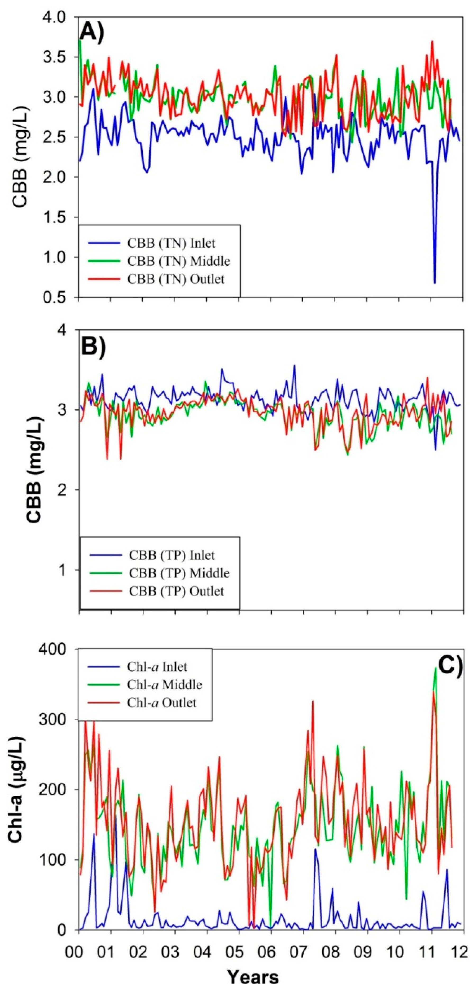
Figure 3 shows the results of the application of both equations for the three sampling points for the estimation of CBB. Based on TN, Figure 3A shows a lower CBB concentration at the inlet (blue line) as compared with that at the middle (green line) and the outlet (red line). Figure 3B represents the CBB estimation based on TP, which shows the TP trend line at the inlet (blue line) being the highest during most of the study period. For both cases, an estimation of CBB concentration for any time point with TN and/or TP data was observed. Since we do not have in situ data for cyanobacteria, these results, together with the data on chl-a concentrations (Figure 3C) and the history of cyanobacteria bloom in the lake, strongly suggest the presence of cyanobacteria.
Figure 3. Time series of cyanobacteria biomass (CBB) estimations from (A) TN and (B) TP at the three sampling points, (C) data on measured chl-a concentrations.
Ijgi 03 01234 g003
However, Figure 3A,B shows different patterns for the cyanobacteria presence among the three regions. Figure 3A, based on Equation (2), showed a lower CBB at the inlet as compared with the other two monitoring sites, while Figure 3B shows the opposite. To better evaluate the presence of cyanobacteria in Lake Thonotosassa, we analyzed the TN: TP ratio (shown in Table 3), since TN:TP ratios have been associated with the concentration of cyanobacteria in lake water [5]. Although it has been proposed that low ratios of TN:TP lead to a higher cyanobacteria concentration [39,40], the opposite case has also been proposed, where low ratios of TN:TP may rather be the result of a high cyanobacteria presence, due to the possible ability of cyanobacteria to pump out phosphorus from enriched sediments [41]. Furthermore, other studies have supported alternative explanations, according to which other factors, such as nutrient variations, rather than low ratios of TN:TP, could be the main triggers of higher cyanobacteria concentration or toxic blooms [42].
In our study case, Table 3 shows the inverse relationship between the trends in TN and TP along the inlet-outlet transect and the direct relationship between the trends of chl-a and TN along it. This could in fact suggest that cyanobacteria are an important contributor in the overall chl-a concentration in the water column of the lake. Such a hypothesis could be explained as a consequence of the well-known ability of cyanobacteria to fix nitrogen [39]. Cyanobacteria would be favored over other species of phytoplankton by conditions of relatively limited nitrogen and abundant phosphorus in the water supply to the lake [43,44]. Depending on nutrient fluxes and the sink capacity of the sediments, it is possible that as water flows from the inlet to the outlet of the lake, the ratio between TN and TP in the water column gradually changes as cyanobacteria uptake TP from the solution and fix nitrogen in solution. Indeed, it can be noticed from Table 3 that both the TN:TP ratio and the chl-a concentration are lowest at the inlet, presumably because at that site, the inflow water with the lowest TN:TP ratio has just entered the lake and has not had enough retention time yet to affect the cyanobacteria; thus, the chl-a concentration is low. The middle and outlet sites monitor lake water with a longer retention time; thus, there is a longer opportunity for cyanobacteria to increase in abundance by taking advantage of the still low TN:TP ratio. Although such a ratio has increased by the time the water reaches the middle and outlet, it is still low and, therefore, still nitrogen limiting and, consequently, favorable for cyanobacterial growth. This could explain the higher chl-a concentration at the middle and outlet sites.
According to the nutrient limitation criteria suggested by Brezonik [45] and the results of Table 3, Lake Thonotosassa is a nitrogen-limited environment. Such criteria propose that lakes with TN:TP ratios less than 10 are nitrogen-limited, while those lakes with ratios greater than 30 are phosphorus-limited, and those ranging between 10 and 30 are balanced (both nutrients are limiting). This, along with the episodic blooms of cyanobacteria reported at the lake [21], agree with the associations reported in the literature between cyanobacteria and low TN:TP ratios [5,40]. Furthermore, the fact that both the TN: TP ratio and chl-a concentration increase together from the inlet to the middle does not coincide with the proposition of Xie et al. [41] that a low TN:TP ratio is a result of a high cyanobacteria concentration, in which case, a lower TN:TP ratio would be expected with more chl-a.
It seems plausible that the TN:TP ratio has indeed an effect on the cyanobacteria in the lake water, which would be mostly the case from the TN:TP ratio of the inflow water [43,44]. This highlights the importance for management plans to focus on the reduction of phosphorus inputs as a way to prevent cyanobacteria blooms and consequent public health issues. As we have indicated, since it is highly plausible that in our study case that the chl-a is importantly composed of cyanobacteria, the importance of monitoring chl-a in a more consistent manner as a way to monitor the effectiveness of such management plans is evident.

3.2. Ocean Color Algorithms Performances

Figure 4 shows the application results from the three algorithms, used for comparison, in a MODIS-Aqua L0 image acquired on 14 April 2006, over the State of Florida. As expected, none of the three algorithms were able to retrieve chl-a concentrations from Lake Thonotosassa. The OC3M was the only algorithm that could perform chl-a estimation in the MODIS L0 product (Figure 4). However, such an estimation was not useful for inland aquatic systems, mainly due to the size of the water body and consequent issues with spatial resolution. Accordingly, this algorithm has been reported previously to be able to retrieve some variation of chl-a in Tampa Bay, Florida, a body of water covering about 1000 km2 at a high tide, but even in that case, its performance was considerably lower as compared with a 1-km spatial resolution MODIS chlorophyll fluorescence line height (FLH) product [18]. The use of GSM and GIOP could not retrieve any spatial variation of the chl-a concentration. These results agree with those found by Tilstone et al. [46], who evaluated the same algorithms for the eastern Arabian Sea coast and similarly found that OC3M had the best performance among the same three algorithms. These observations highlight the need to develop water quality products with a higher spatial resolution for the study and monitoring of small aquatic systems.
Figure 4. OC3M application using SeaDAS 7.02 on a MODIS-Aqua L0 product.
Ijgi 03 01234 g004

3.3. Locally-Tuned Algorithm

3.3.1. Band Selection

Upon confirming the unsatisfactory results from the MODIS-Aqua L0 1-km product, we used the MOD09GA product with a spatial resolution of 500 m to develop empirical models. However, the single spectral bands from the MOD09GA product were not suitable for water color studies either, since they cannot detect the small spectral variations required [14]. We compared chl-a concentration against MOD09GA reflectance to analyze their relationship using the reflectance from single bands. Table 4 shows the correlation for each spectral band of MOD09GA (days without cloud cover over Lake Thonotosassa) to the chl-a concentration per period of the year using the calibration dataset. As shown in Table 4, algorithms based on a single band were not useful for estimating the chl-a concentration in Lake Thonotosassa during the last six months of the year.
Table 4. Coefficient of determination (R2) for chl-a (μg/L) and reflectance values from each band for four periods of the year: January to March (JFM), April to June (AMJ), July to September (JAS) and October to December (OND).
JFMAMJJASOND
Band 1 (620–670 nm)0.070.670.000.00
Band 2 (841–876 nm)0.000.710.010.01
Band 3 (459–479 nm)0.150.620.010.00
Band 4 (545–565 nm)0.250.580.000.00
Band 5 (1230–1250 nm)0.030.670.000.01
Band 6 (1628–1652 nm)0.020.700.000.00
Band 7 (2105–2155 nm)0.010.710.000.01
Different spectral bands were found to be the most correlated for each period. The highest correlations were observed in the April to June (AMJ) period, which is also the period of the year with higher chl-a concentrations (179.36 μg/L). For the periods with a low chl-a concentration, July to September (JAS) (126.83 μg/L) and October to December (OND) (132.12 μg/L), the R2 was low. Finally, the January to March (JFM) period, which presented a higher R2 as compared to JAS and OND, but lower R2 as compared to AMJ, presented a chl-a concentration greater than that of JAS and OND, but lower than that of AMJ (148.49 μg/L). These observations demonstrate the need for seasonal calibrations of the empirical algorithms.
To understand the physical principles behind the algorithm development, we plotted the average reflectance spectrum for each period (Figure 5). No relationship between chl-a concentration and the reflectance peak at Band 2 (in the NIR) was observed. The highest reflectance value was detected in the OND period, with an average chl-a concentration of 132.12 μg/L, followed in order by the JAS, AMJ and JFM periods with average chl-a concentrations of 126.83 μg/L, 179.36 μg/L and 148.49 μg/L, respectively. It was concluded from this lack of correlation that single bands were not useful for the estimation of chl-a concentration.
As a next step, band ratios among the seven spectral bands were tested. The importance of using band ratios lies in the fact that the specular reflection from water under wavy conditions gets suppressed by the ratio architecture of this type of algorithm, which cancels out the specular reflection from the two bands used in the ratio [47]. To analyze all possible band ratios, we used the ICE [37] to generate two-dimensional correlation plots of the R2 between chl-a concentration and band ratio values. ICE was previous described in Section 2.4.1, and more information can be found in [37]. Figure 6 shows the plots for the four seasons analyzed using the calibration dataset.
As shown by the four 2D correlation plots in Figure 6, the best performances are obtained from the ratio between Band 1 and Band 4 or Band 4 and Band 1 (the highest R2 on the 2D color correlation plot for all of the periods; Figure 6A–D). Band 1 is located in the red channel around 675 nm, where there is an important chl-a absorption feature. Another reflectance peak of chl-a is located at Band 4 in the green channel around 550 nm. With attention to this, the algorithm we proposed here for all four seasons is shown in Equation (4):
C h l a B 1 B 4 B 1 + B 4
where B1 is related to MOD09GA reflectance from spectral Band 1 and B4 is related to MOD09GA reflectance from spectral Band 4.
Figure 5. Average reflectance spectra of MOD09GA for each seasonal period.
Ijgi 03 01234 g005
Figure 6. 2D correlation plots of MOD09GA spectral bands using ICE [37]. (A) JFM; (B) AMJ; (C) JAS; (D) OND.
Ijgi 03 01234 g006

3.3.2. Calibration and Validation

The algorithm was seasonally calibrated using MOD09GA data from 2000 to 2007. A linear calibration was performed for each period to retrieve its slope and intercept. Table 5 shows the calibrations coefficients, indicating an average performance for most of the periods, with R2 of 0.53, 0.56 and 0.67 for the JFM, AMJ and JAS periods, respectively. Nevertheless, a clearly lower R2 (0.06) was detected for the linear calibration in the OND period.
Table 5. Calibration coefficients for the algorithm for each period.
R2SlopeInterceptp-Value
JFM0.53−426.81144.780.003
AMJ0.56−289.51137.720.008
JAS0.67357.46137.180.012
OND0.06−148.15125.870.440
It can be observed from the 2D correlation plots in Figure 6 that the relationship between reflectance and chl-a concentration in the OND period did not present any R2 higher than 0.08. The same was observed by applying the proposed algorithm with a very low R2 with a very high p-value (0.440). As can be appreciated from Table 5 and Figure 7, the models were better calibrated for the first three periods: JFM, AMJ and JAS. Figure 7C shows a positive slope during the JAS period, while all of the others figures (Figure 7A–C for periods JFM, AMJ and OND, respectively) present a negative slope. Such a negative slope can be explained by the algorithm structure, which is sensitive to the absorption of phytoplankton in the red channel, as well as the phytoplankton reflectance peak in the green channel. Conversely, a positive slope indicates an increase in the signal in the red channel, which is related to a cyanobacteria pigment known as phycocyanin (PC) with a fluorescence peak at 650 nm. Such a fluorescence peak is close to the center of MODIS Band 1. This circumstance causes an increase in the signal of this band at high cyanobacteria concentrations. Moreover, the JAS period is usually related to the summer, where several cyanobacteria cases are reported mainly due to the high temperature observed in this season.
The linear calibrations depicted in Figure 7 were used in the validation process with MOD09GA data, which covered the period from 2008 to 2011. The coefficients of the calibration (slope and intercept from Table 5) were applied on the surface reflectance data derived from the MOD09GA product. The error estimators in Table 2 were used to evaluate the performance of the model. Table 6 shows the error estimators for the four periods of the year.
Table 6. Errors estimators used in the validation dataset for each period.
JFMAMJJASOND
Bias38.5891.4652.9425.53
NBias0.230.270.461.74
RMSE45.2112.0862.0227.16
NRMSE0.270.340.541.85
The variation in the error estimator from period to period of each year can be appreciated in Table 6. Both NBias and NRMSE indicated lower error estimators for the periods with higher chl-a concentrations (JFM and AMJ) as compared with those periods with lower chl-a concentrations (JAS and OND). These errors could be related to the atmospheric correction of the MOD09GA product, which is based on the utilization of look-up tables (LUTs) of top of atmosphere (TOA) reflectance values [48]. This is needed to retrieve surface reflectance properties on the basis of given TOA reflectance values and atmospheric parameters [48]. Hence, the accuracy of using MOD09GA depends on several aspects, such as the accuracy of sensor calibration, input atmospheric parameters, LUTs and operational implementation of correction for bidirectional reflectance distribution function effects [49]. More details about the atmospheric correction used in the MOD09GA product can be found in Vermote et al. [48]. The NRMSE results, though, agree with Cowell et al. [22], which identified more abundant green algae (Chlorophyceae) in Lake Thonotosassa during the spring and early summer months, while blooms of blue-green algae (mainly Anabaena spiroides) were during the summer. This phytoplankton dynamic enhanced the accuracy for the first two trimesters, which received lower errors. During the third and fourth trimester, Cowell et al. [22] identified the occurrence of diatom blooms (mainly Stephanodiscus hantzschii). This could explain the high errors, since diatoms have a different spectral shape with higher reflectance values, and their steep spectrum decreases from 412 to 510 nm [50]. As shown by Ogashawara et al. [14], this range of estimator errors for chl-a concentration estimation from a MOD09GA product is reasonable. This assumption is mainly based on the spectral resolution of the seven first MODIS bands, which were not the ideal for water color studies, since they are not able to collect the signal from important sections of the water leaving radiance spectra.
Figure 7. Linear regression plots of the calibration between model values and chl-a concentration for each period of the year. (A) JFM; (B) AMJ; (C) JAS; (D) OND.
Ijgi 03 01234 g007
Moreover, several studies using more appropriate MODIS spectral bands for water color analysis still have presented similar or poorer error estimator results. Le et al. [51] used MODIS Bands 11 (526–536), 12 (546–556) and 14 (673–683), which have a narrow range that meets the chl-a-specific spectral range of reflectance and absorption. Using these spectral bands, the authors produced an RMSE (%) of 36.5%, and they also attributed a value of 39.6% of the error to the red-green ratio algorithms as acceptable for estuaries.

3.4. Possible Applications

The development of empirical algorithms for the monitoring of chl-a concentration for Lake Thonotosassa can lead to several environmental and public health applications. Ogashawara et al. [14] demonstrated the usefulness of applying empirical algorithms to retrieve a time-series of chl-a concentration to improve the monitoring in regions with a considerable lack of data acquisition. Although Lake Thonotosassa is monitored monthly, the possibility of having more frequent data is important, because water quality parameters can change rapidly. Furthermore, a monitoring method based on fixed locations may not be representative of the mean chl-
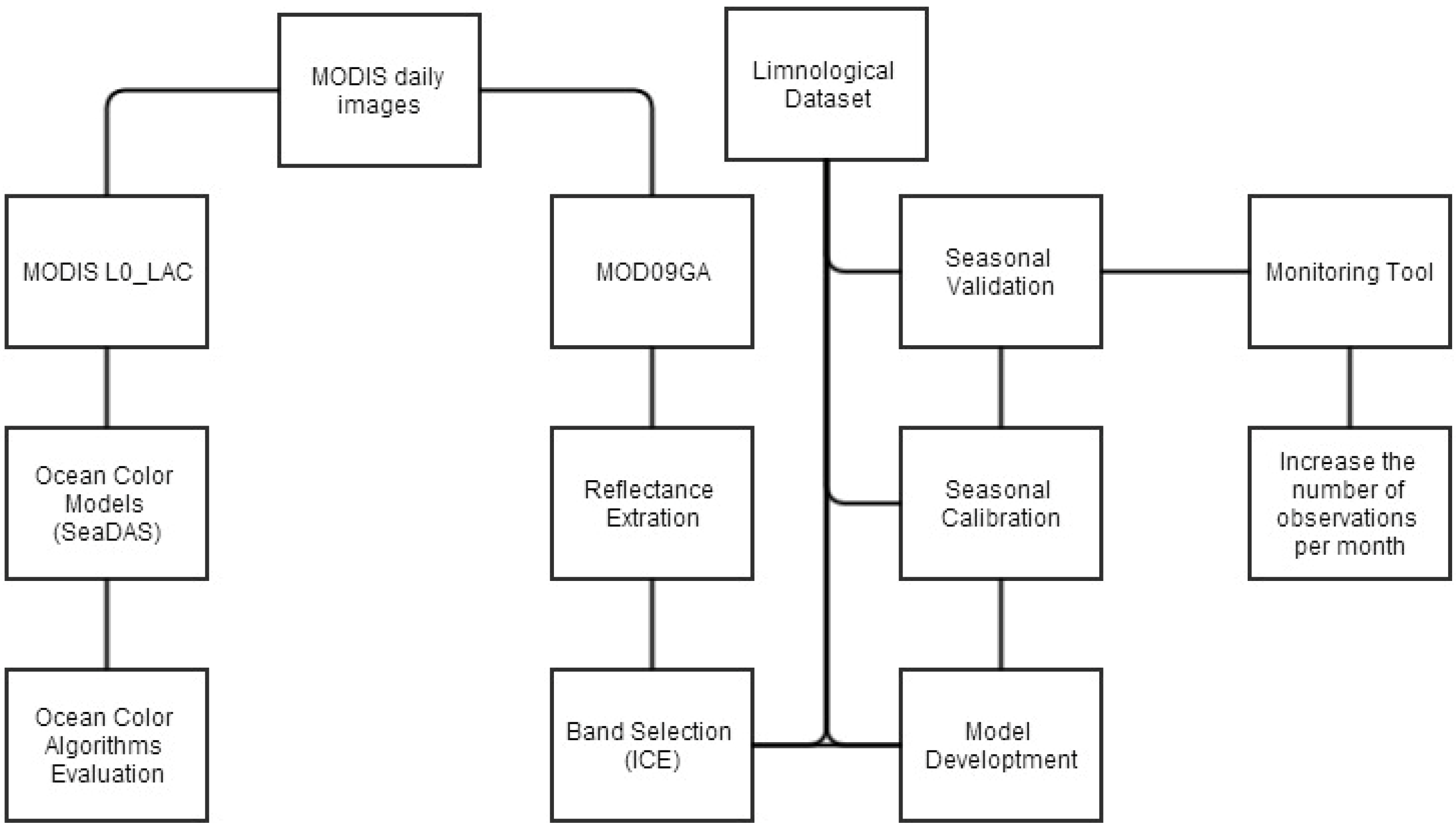
a concentration in the lake, as other locations of potential interest within the lake are not considered. Thus, the use of MOD09GA, which is a daily product, can improve the frequency of monitoring water quality, mainly algal blooms, further providing the feasibility to cover areas within the lake not included in the routine monitoring plan. As indicated by calculations according to Beaulieu et al. [38] and by the analysis of in situ data for TN:TP ratios, there is an important indication that cyanobacteria are a core component of the chl-a present in Lake Thonotosassa. As growing populations in urban and suburban areas increasingly rely on lakes for ecosystem services, such as recreation, aesthetics, culture and storm-water drainage and treatment [1,52], the use of practical time- and cost-effective methodologies to monitor water quality is accordingly becoming more imperative. The risk of cyanobacteria presence in urban lakes and consequent potential danger to public health amply justify the implementation of water quality monitoring programs. These programs are important, since human intoxication from cyanotoxins, such as microcystin, does not occur only through the ingestion of drinking water or food. It can also occur through recreational dermal contact during aquatic activities, such as practicing aquatic sports, bathing, swimming and diving [53]. Moreover, these activities also promote accidental ingestion of water, which is a concern, since ingestion of even a small quantity of cyanotoxins can have serious health consequences [54]. Therefore, in a broader scope, chl-a monitoring in general is an increasingly important need. The web tool procedures and remote sensing techniques used in this study were shown to be useful for applications to water chl-a monitoring or algal bloom identification in Lake Thonotosassa. Furthermore, the proposed approach and procedures can also be applied to develop customized remote sensing methodologies in other lakes with similar environmental conditions. This initiative can improve local water governance systems, as well as can be an important tool for environmental and public health managers. Additionally, the community as the major stakeholders could be trained in the use of remote sensing technology to be involved in the monitoring process in a sustainable low-cost approach.

4. Conclusions

Our analysis of in situ data of the changes in TN: TP ratios and chl-a concentration along the flow transect covering the three monitoring sites suggests the presence of cyanobacteria in Lake Thonotosassa. To validate these findings, an analysis through the TN and TP relations established by Beaulieu et al. [38] along with chl-a concentration highlighted the presence of cyanobacteria. Considering that some cyanobacteria species have the ability to produce toxins (which can be dangerous to human health through different routes of entry) along with the potential risk of exposure (as this lake is located in a suburban area and discharges into the Hillsborough River, which is the main source of municipal water supply for the City of Tampa), the importance of implementing monitoring programs in this water body is clear. Such a practice could anticipate and prevent related health issues in the community interacting with the lake.
Remote sensing techniques, such as bio-optical modeling, are an alternative to qualitatively monitoring of biological activity through chl-a concentration. Using MODIS-Aqua L0 products and SeaDAS, we implemented three ocean color algorithms that resulted in non-suitable products, due to the use of spectral bands with low spatial resolution, which were unable to identify small water bodies. Since they are global algorithms and originally modeled for oceanic waters, our empirical model especially designed for a small inland lake was shown to improve the results. We used MOD09GA (500 m) data to develop an empirical chl-a bio-optical model based on the band selection provided by 2D color correlation plots of R2 between band ratios and measured chl-a concentration. We grouped 11 years of MOD09GA data by trimester and calibrated the algorithm for each of these time periods. The NRMSE for the first trimester of the year was 0.27, while for the second, third and fourth trimester, it was 0.34, 0.54 and 1.85, respectively. These results showed a greater error during the fourth trimester of the year, as compared with the other trimesters. This is probably explained by the presence of diatoms during this period of time, which shows the need for the development of filters to remove the effect of others water constituents. We also highlight here the need for seasonal calibration of bio-optical models, as seasonal variability in the aquatic system can change the environment dynamics. Thus, we have shown the applicability of remote sensing techniques to monitor water quality, even in small water bodies, such as Lake Thonotosassa. Nevertheless, it is clear that the understanding of environmental factors and their effects on seasonal variations are crucial for better algorithm calibration.
Although the spatial resolution from MODIS products is often not suitable for small water bodies, it is still possible to acquire daily data to retrieve a long-term time-series from one pixel that fits the required conditions. This can be useful to monitor the effects on water quality from human activities in the watershed and the progress of environmental management plans aimed at improving water quality. This improvement is needed, since an adequate monitoring system for aquatic environments may imply high costs that make difficult its implementation difficult. Moreover, immediate management options should be available to provide information for the population, especially for those who depend on the aquatic environment. Remote sensing techniques showed here a high potential for the environmental and public health management of inland aquatic systems. MODIS products constitute a great help in understanding environmental dynamics in order to propose better environmental and health policies concerning water resources. Thus, remote sensing can be an important tool for environmental decision makers, which will influence the environment and human health.

Acknowledgments

The authors express their appreciation to the Environmental Protection Commission of Hillsborough County (EPCHC) for providing the in situ water quality data and, particularly, to Rick Garrity and Richard Boler for facilitating the process of data sharing. MODIS data collection and processing were made possible through the efforts of MODIS Adaptive Processing System (MODAPS) services at the NASA Goddard Space Flight Center (NASA/GSFC) and NASA’s Earth Observing System Data and Information System (NASA/EOSDIS). Also acknowledged is the SeaDAS Development group at NASA GSFC for the use of the SeaDAS software to process the MODIS imagery. Special acknowledgment is given to Steve Padgett Vasquez for introducing the authors.

Author Contributions

Igor Ogashawara and Max J. Moreno-Madrinan conceived of and designed the paper together. Igor Ogashawara is the main author of the paper, who performed the RS analyses. Igor Ogashawara and Max J. Moreno-Madriñán equally participated in the writing of the manuscript and limnological analysis. Max J. Moreno-Madriñán classified the in-situ dataset and revised the entire manuscript.

Conflicts of Interest

The authors declare no conflict of interest.

References

  1. Rodríguez, J.P.; Beard, T.D., Jr.; Bennett, E.M.; Cumming, G.S.; Cork, S.J.; Agard, J.; Dobson, A.P.; Peterson, G.D. Trade-offs across space, time, and ecosystem services. Ecol. Soc. 2006, 11, 1–14. [Google Scholar]
  2. Pitois, S.; Jackson, M.H.; Wood, B.J. Sources of the eutrophication problems associated with toxic algae: An overview. J. Environ. Health 2001, 64, 25–32. [Google Scholar] [PubMed]
  3. Mudroch, A. (Ed.) Planning and Management of Lakes and Reservoirs, An Integrated Approach to Eutrophication; UNEP International Environmental Technology Centre: Osaka, Japan, 1999.
  4. O’Neil, J.M.; Davis, T.W.; Burford, M.A.; Gobler, C.J. The rise of harmful cyanobacteria blooms: The potential roles of eutrophication and climate change. Harmful Algae 2012, 14, 313–334. [Google Scholar] [CrossRef]
  5. Kotak, B.G.; Zurawell, R.W. Cyanobacterial toxins in Canadian freshwaters: A review. Lake Reserv. Manag. 2007, 23, 109–122. [Google Scholar] [CrossRef]
  6. Fleming, L.E.; Rivero, C.; Burns, J.; Williams, C.; Bean, J.A.; Shea, K.A.; Stinn, J. Blue green algal (cyanobacterial) toxins, surface drinking water, and liver cancer in Florida. Harmful Algae 2002, 1, 157–168. [Google Scholar] [CrossRef]
  7. Francis, G. Poisonous Australian Lake. Nature 1878. [Google Scholar] [CrossRef]
  8. Azevedo, S.M.F.O.; Carmichael, W.W.; Jochimsen, E.M.; Rinehart, K.L.; Lau, S.; Shaw, G.R.; Eaglesham, G.K. Human intoxication by microcystins during renal dialysis treatment in Caruaru—Brazil. Toxicology 2002, 181–182, 441–446. [Google Scholar] [CrossRef] [PubMed]
  9. Centers for Disease Control and Prevention (CDC). Recreational Water—Associated Disease Outbreaks—United States, 2009–2010. Available online: http://www.cdc.gov/mmwr/preview/mmwrhtml/mm6301a2.htm?s_cid=mm6301a2_w (accessed on 8 May 2014).
  10. Jogensen, S.E.; Bendoricchio, G. Fundamentals of Ecological Modeling, 3rd ed.; Elsevier: New York, NY, USA, 2001. [Google Scholar]
  11. Dall’Olmo, G.; Gitelson, A.A.; Rundquist, D.C.; Leavitt, B.; Barrow, T.; Holz, J.C. Assessing the potential of SeaWiFS and MODIS for estimating chlorophyll concentration in turbid productive waters using red and near-infrared bands. Remote Sens. Environ. 2005, 96, 176–187. [Google Scholar] [CrossRef]
  12. Le, C.; Li, Y.; Zha, Y.; Sun, D.; Huang, C.; Lu, H. A four-band semi-analytical model for estimating chlorophyll a in highly turbid lakes: The case of Taihu Lake, China. Remote Sens. Environ. 2009, 113, 1175–1182. [Google Scholar] [CrossRef]
  13. Hadjimitsis, D.G.; Clayton, C. Assessment of temporal variations of water quality in inland water bodies using atmospheric corrected satellite remotely sensed image data. Environ. Monit. Assess. 2009, 159, 281–292. [Google Scholar] [CrossRef] [PubMed]
  14. Ogashawara, I.; Alcântara, E.H.; Curtarelli, M.P.; Adami, M.; Nascimento, R.F.F.; Souza, A.F.; Stech, J.L.; Kampel, M. Performance analysis of MODIS 500-m spatial resolution products for estimating Chlorophyll-a concentrations in Oligo- to Meso-Trophic waters case study: Itumbiara Reservoir, Brazil. Remote Sens. 2014, 6, 1634–1653. [Google Scholar] [CrossRef]
  15. Gitelson, A.; Garbuzov, G.; Szilagyi, F.; Mittenzwey, K.H.; Karnielli, A.; Kaiser, A. Quantitative remote sensing methods for real-time monitoring of inland waters quality. Int. J. Remote Sens. 1993, 14, 1269–1295. [Google Scholar] [CrossRef]
  16. Gons, H.J. Optical teledetection of chlorophyll a in turbid inland waters. Environ. Sci. Technol. 1999, 33, 1127–1132. [Google Scholar] [CrossRef]
  17. Moses, W.J.; Gitelson, A.A.; Berdnikov, S.; Bowles, J.H.; Povazhnyi, V.; Saprygin, V.; Wagner, E.J.; Patterson, K.W. HICO-based NIR-Red models for estimating Chlorophyll-a concentration in productive coastal waters. IEEE Geosci. Remote Sens. 2014, 11, 1111–1115. [Google Scholar] [CrossRef]
  18. Moreno-Madriñán, M.J.; Fischer, M.A. Performance of the MODIS FLH algorithm in estuarine waters: A multi-year (2003–2010) analysis from Tampa Bay, Florida (USA). Int. J. Remote Sens. 2013, 34, 6467–6483. [Google Scholar] [CrossRef]
  19. Dall’Olmo, G.; Gitelson, A.A. Effect of bio-optical parameter variability on the remote estimation of chlorophyll-α concentration in turbid productive waters: Experimental results. Appl. Opt. 2005, 44, 412–422. [Google Scholar] [CrossRef] [PubMed]
  20. Dall’Olmo, G.; Gitelson, A.A. Effect of bio-optical parameter variability and uncertainties in reflectance measurements on the remote estimation of chlorophyll-α concentration in turbid productive waters: Modeling results. Appl. Opt. 2006, 45, 3577–3592. [Google Scholar] [CrossRef] [PubMed]
  21. Southwest Florida Water Management District. Lake Thonotosassa Surface Water Improvement and Management (SWIM) Plan; Southwest Florida Water Management District: Plant City, FL, USA, 2003.
  22. Cowell, B.C.; Dye, C.W.; Ada, R.C. A synoptic study of the limnology of Lake Thonotosassa, Florida. Part I. effects of primary treated sewage and citrus wastes. Hydrobiologia 1975, 46, 301–345. [Google Scholar] [CrossRef]
  23. Cowell, B.C.; Vodopich, D.S. Distribution and seasonal abundance of benthic macroinvertebrate in a subtropical Florida lake. Hydrobiologia 1981, 78, 97–105. [Google Scholar] [CrossRef]
  24. Florida Department of Environmental Regulation. Integrated Water Quality Assessment for Florida: 2012 305(b) Report and 303(d) List Update; Florida Department of Environmental Regulation—Division of Environmental Assessment and Restoration: Tallahassee, FL, USA, 2012. [Google Scholar]
  25. Clesceri, L.S.; Eaton, A.D.; Greenberg, A.E.; Franson, M.A.H. (Eds.) Standard Methods for the Examination of Water and Wastewater; American Public Health Association, American Water Works Association & Water Environment Federation: Washington, DC, USA, 1998.
  26. Moreno-Madriñán, M.J. Analysis of limnological variables associated to water quality in lakes of Northwestern Hillsborough County, Florida. Fla. Sci. 2010, 73, 218–224. [Google Scholar]
  27. Moreno-Madriñán, M.J. Analysis of the relationship between Submerged Aquatic Vegetation (SAV) and water trophic status of lakes clustered in Northwestern Hillsborough County, Florida. Water Air Soil Poll. 2011, 214, 539–546. [Google Scholar] [CrossRef]
  28. Ocean Color Web. Available online: http://oceancolor.gsfc.nasa.gov/ (accessed on 3 February 2014).
  29. EOS ClearingHouse (ECHO). Available online: http://reverb.echo.nasa.gov/ (accessed on 3 February 2014).
  30. Fu, G.; Settle, K.; McClain, C.R. SeaDAS: The SeaWiFSData analysis system. In Proceedings of the 1998 Pacic Ocean Remote Sensing Conference, Qingdao, China, 28–31 July 1998; Secretariat: Beijing, China, 1998; pp. 73–77. [Google Scholar]
  31. O’Reilly, J.E.; Maritorena, S.; O’Brien, M.C.; Siegel, D.A.; Toole, D.; Menzies, D.; Smith, R.C.; Mueller, J.L.; Mitchell, B.G.; Kahru, M.; et al. SeaWiFS Postlaunch Calibration and Validation Analyses; Part 3, Volume 11; National Aeronautics and Space Administration: Washington, DC, USA, 2000.
  32. Maritorena, S.; Siegel, D.A.; Peterson, A.R. Optimization of a semianalytical ocean color model for global-scale applications. Appl. Opt. 2002, 41, 2705–2714. [Google Scholar] [CrossRef] [PubMed]
  33. Franz, B.A.; Werdell, P.J. A generalized framework for modeling of inherent optical properities in ocean remote sensing applications. In Proceedings of the 2010 Ocean Optics, Anchorage, AK, USA, 27 September–1 October 2010.
  34. Morel, A. Optical modeling of the upper ocean in relation to its biogenous matter content (case I waters). J. Geophys. Res. 1988, 931, 10749–10768. [Google Scholar] [CrossRef]
  35. Gordon, H.R. Ocean color remote sensing: Influence of the particle phase function and the solar zenith angle. EOS Trans. Am. Geophys. Union 1986, 14, 1055. [Google Scholar]
  36. Ruddick, K.; Ovidio, F.; Rijkeboer, M. Atmospheric correction of SeaWiFS imagery for turbid coastal and inland waters. Appl. Opt. 2000, 39, 897–912. [Google Scholar] [CrossRef] [PubMed]
  37. Ogashawara, I.; Curtarelli, M.P.; Souza, A.F.; Augusto-Silva, P.B.; Alcântara, E.H.; Stech, J.L. Interactive Correlation Environment (ICE)—A statistical web tool for data collinearity analysis. Remote Sens. 2014, 6, 3059–3074. [Google Scholar] [CrossRef]
  38. Beaulieu, M.; Pick, F.; Gregory-Eaves, I. Nutrients and water temperature are significant predictors of cyanobacterial biomass in a 1147 lakes data set. Limnol. Oceanogr. 2013, 58, 1736–1746. [Google Scholar] [CrossRef]
  39. Smith, V.H. Low nitrogen to phosphorus ratios favor dominance by blue-green algae in lake phytoplankton. Science 1983, 221, 669–671. [Google Scholar] [CrossRef] [PubMed]
  40. Orihel, D.M.; Bird, D.F.; Brylinsky, M.; Chen, H.; Donald, D.B.; Huang, D.Y.; Giani, A.; Kinniburgh, D.; Kling, H.; Kotak, B.G.; et al. High microcystin concentrations occur only at low nitrogen-to-phosphorus ratios in nutrient-rich Canadian lakes. Can. J. Fish. Aquat. Sci. 2012, 69, 1457–1462. [Google Scholar] [CrossRef]
  41. Xie, L.; Xie, P.; Li, S.; Tang, H.; Liu, H. The low TN:TP ratio, a cause or a result of Microcystis blooms? Water Res. 2003, 37, 2073–2080. [Google Scholar] [CrossRef] [PubMed]
  42. Downing, J.A.; Watson, S.B.; McCauley, E. Predicting Cyanobacteria dominance in lakes. Can. J. Fish. Aquat. Sci. 2001, 58, 1905–1908. [Google Scholar] [CrossRef]
  43. Schindler, D.W. Evolution of phosphorus limitation in Lakes. Science 1977, 195, 260–262. [Google Scholar] [CrossRef] [PubMed]
  44. Schindler, D.W.; Hecky, R.E.; Findlay, D.L.; Stainton, M.P.; Parker, B.R.; Paterson, M.J.; Beaty, K.G.; Lyng, M.; Kasian, S.E.M. Eutrophication of lakes cannot be controlled by reducing nitrogen input: Results of a 37-year whole-ecosystem experiment. Proc. Natl. Acad. Sci. USA 2008, 105, 11254–11258. [Google Scholar] [CrossRef] [PubMed]
  45. Brezonik, P.L. Trophic state indices: Rationale for multivariate approaches. Lake Reserv. Manag. 1984, 1, 441–445. [Google Scholar] [CrossRef]
  46. Tilstone, G.H.; Lotliker, A.A.; Miller, P.I.; Ashraf, P.M.; Kumar, T.S.; Suresh, T.; Ragavan, B.T.; Menon, H.B. Assessment of MODIS-Aqua chlorophyll-α algorithms in coastal and shelf waters of the eastern Arabian Sea. Cont. Shelf Res. 2013, 65, 14–26. [Google Scholar] [CrossRef]
  47. Vincent, R.K.; Qin, X.; McKay, R.M.L.; Miner, J.; Czajkowski, K.; Savino, J.; Bridgeman, T. Phycocyanin detection from LANDSAT TM data for mapping cyanobacterial blooms in Lake Erie. Remote Sens. Environ. 2004, 89, 381–392. [Google Scholar] [CrossRef]
  48. Vermote, E.F.; El Saleous, N.Z.; Justice, C.O. Atmospheric correction of visible to middle-infrared EOS-MODIS data over land surfaces: Background, operational algorithm and validation. J. Geophys. Res. 1997, 102, 17131–17141. [Google Scholar] [CrossRef]
  49. Vermote, E.F.; Kotchenova, S. Atmospheric correction for the monitoring of land surfaces. J. Geophys. Res. 2008, 113. [Google Scholar] [CrossRef]
  50. Alvain, S.; Moulin, C.; Dandonneau, Y.; Bréon, F.M. Remote sensing of phytoplankton groups in case 1 waters from global SeaWiFS imagery. Deep Sea Res. I 2005, 52, 1989–2004. [Google Scholar] [CrossRef] [Green Version]
  51. Le, C.; Hu, C.; English, D.; Cannizzaro, J.; Chen, Z.; Feng, L.; Boler, R.; Kovach, C. Towards a long-term chlorophyll-α data record in a turbid estuary using MODIS observations. Prog. Oceanogr. 2012, 109, 90–103. [Google Scholar] [CrossRef]
  52. Bolund, P.; Hunhammar, S. Ecosystem services in urban areas. Ecol. Econ. 1999, 29, 293–301. [Google Scholar] [CrossRef]
  53. Chorus, I.; Bartram, J. Toxic Cyanobacteria in Water: A Guide to Their Public Health Consequences, Monitoring and Management; UNESCO/WHO/UNEP: London, UK, 1999. [Google Scholar]
  54. World Health Organization. Guidelines for Safe Recreational Water Environments, Volume I: Coastal and Fresh Waters; World Health Organization: Geneva, Switzerland, 2003. [Google Scholar]

