Dynamically Integrating OSM Data into a Borderland Database

Abstract

Spatial data are fundamental for borderland analyses of geography, natural resources, demography, politics, economy, and culture. As the spatial data used in borderland research usually cover the borderland regions of several neighboring countries, it is difficult for anyone research institution of government to collect them. Volunteered Geographic Information (VGI) is a highly successful method for acquiring timely and detailed global spatial data at a very low cost. Therefore, VGI is a reasonable source of borderland spatial data. OpenStreetMap (OSM) is known as the most successful VGI resource. However, OSM's data model is far different from the traditional geographic information model. Thus, the OSM data must be converted in the scientist’s customized data model. Because the real world changes rapidly, the converted data must be updated incrementally. Therefore, this paper presents a method used to dynamically integrate OSM data into the borderland database. In this method, a basic transformation rule base is formed by comparing the OSM Map Feature description document and the destination model definitions. Using the basic rules, the main features can be automatically converted to the destination model. A human-computer interaction model transformation and a rule/automatic-remember mechanism are developed to interactively transfer the unusual features that cannot be transferred by the basic rules to the target model and to remember the reusable rules automatically. To keep the borderland database current, the global OsmChange daily diff file is used to extract the change-only information for the research region. To extract the changed objects in the region under study, the relationship between the changed object and the research region is analyzed considering the evolution of the involved objects. In addition, five rules are determined to select the objects and integrate the changed objects with multi-versions over time. The objects’ change-type evolution is analyzed, and seven rules are used to determine the change-type of the changed objects. Based on these rules and algorithms, we programmed an automatic (or semi-automatic) integrating and updating prototype system for the borderland database. The developed system was intensively tested using OSM data for Vietnam and Pakistan as the experimental data.

1. Introduction

Spatial data are fundamental for borderland analyses of geography, natural resources, demography, politics, economy, culture, etc. Because the spatial data used in borderland research usually covers the borderland regions of several neighboring countries, it is difficult for anyone research institution or government to collect. During the past several years, interest in Volunteered Geographic Information (VGI), which is also known as crowdsourcing data, has rapidly grown. VGI is a very successful method for acquiring timely and detailed global spatial data at low cost. Therefore, VGI is one reasonable source of borderland spatial data [1]. However, VGI is voluntarily produced by amateurs (or “neogeographers”) without strict regulation or formal training. VGI usually contains the following limitations: (1) spurious or low-quality data and (2) irregularity in its completeness. These limitations impact VGI’s fitness for use. For borderland analysis, these limitations must be overcome. A reasonable method for overcoming these limitations would be to integrate low-cost VGI with another source of professional data to improve its completeness, remove the spurious or low-quality data, and incrementally update the data. However, the data model of VGI generally differs from the traditional Geographic Information System (GIS) user model. For example, OpenStreetMap (OSM) is known as the most successful VGI project. However, OSM’s geometric primitives include node, way, and relation rather than point, line and polygon, as in the traditional GIS model. All types of streets and paths are identified by a vague “highway” tag, which is much different than traditional geographic information and common sense. Furthermore, because OSM data are collected by a free tagging system, many unusual features are tagged by neogeographers based on their communication habits. Some OSM data can be downloaded in shapefile formatted databases from company websites (e.g., Geofabrik); however, the derived shapefile is a selection of features and attributes of original OSM data. Accordingly, many unusual features are unavailable in the derived shapefile, all of the complex area features are missing [2] and the derived snapshot data cannot be updated incrementally. Therefore, the original OSM data and the derived shapefile from the OSM data cannot satisfy the application requirements to dynamically integrate borderland research. To solve this problem, we present a dynamic integration method for a borderland database using OSM data. In this method, we transfer the OSM crowdsourcing data into a user-data model; that is, we transfer the features to suitable classes with user-defined codes using a rule-based method. To convert unusual features into suitable classes automatically or semi-automatically, an automatic-remember mechanism is presented to assign OSM features to user classes interactively and to automatically remember this transferred knowledge as a rule. The new remembered rules can be reused in later transformations. Using this method, the model transformation rules can be increased incrementally. Using this rule-based data model method of transformation, a snapshot of the research borderland area can be obtained for a particular time. However, for borderland applications, the snapshot map from OSM is usually not sufficient, and scientists often must integrate another source of data to form a suitable database. However, the real world is changing fast and it is necessary to incrementally update the database for the research borderland area. VGI will continue to be a low-cost, worldwide and timely change-only information resource. However, OSM does not provide methods to download the change file for a given region over a particular period. Instead, it only provides global daily diff data in OsmChange. Thus, a method has been developed that extracts the change objects in a given region from the global daily diff data, picks the coordinates for the objects in the regions, and then merges the diff files into one change-only information file with the designed format. Then, the change-only information file is used to automatically update the research borderland database.

This paper is organized into seven sections. In Section 2, we introduce work related to this paper. We discuss the dynamic integration strategy for the borderland database in Section 3. The rule-based model transformation method is described in Section 4. The change-only information extraction method is discussed in Section 5. Experimental tests of this study are presented in Section 6. Finally, Section 7 provides a summary and concludes the discussion.

2. Related Work

In recent years, VGI (or crowdsourcing data) has been a hot issue in GIS research. Researchers primarily focus their work on the following issues: quality evaluation of crowdsourcing data, VGI quality-control methods and the application of VGI.

VGI’s main concern is data quality; therefore, several researchers have evaluated the quality of VGI by comparing OSM data with corresponding professional data. Haklay [3] has examined the data quality for both London and England through a comparison with Ordnance Survey (OS) datasets. Zielstra and Zipf [4] analyzed the completeness of OSM data relative to the navigation data of the TeleAtlas MultiNet datasets in Germany. Girres and Touya [5] completed a quality assessment of France OSM spatial data using the Large-Scale Reference database (RGE) for reference data and a sampling method using the assessment components, i.e., geometric accuracy, attribute accuracy, completeness, logical consistency, semantic accuracy, temporal accuracy, lineage, and usage. Cipeluch et al. compared the accuracy of Ireland OSM data with Google Maps and Bing Maps [6]. Siebritz and Sithole evaluated the quality of OSM data in South Africa by comparing them with a reference data set from national mapping agencies [7]. Forghani and Delavar evaluated the consistency between Tehran, Iran’s OSM dataset and a corresponding reference geospatial dataset [8]. Jackson et al. assessed the completeness and spatial error of features (using the size of school campuses as an example) in the United States (US) [9]. Hecht et al. analyzed the completeness of building footprints in OSM by comparing the OSM data with the official data in Germany [10]; Fan et al. evaluated the quality of OSM building footprint data in terms of completeness, semantic, position and shape accuracy using ATKIS data as reference data [11]. Comber et al. evaluated the reliability of volunteered land cover using GLC-2000, GlobCover and MODIS V5 as control data [12]. In the above analyses, almost all of the researchers concluded that although OSM can offer a large amount of useful data with high responsiveness and flexibility, its main limitation is the irregularity of the data’s completeness.

Unlike professional geographic data, which is collected by trained specialists with specialized standards who guarantee reliability, VGI is collected by non-professional users without specialized training. Accordingly, VGI can contain a great deal of spurious or low-quality data. Therefore, before it can be used in scientific analysis, it is necessary to use some reliability measures to clean or filter spurious or low-quality data. Based on this consideration, several researchers have studied the reliability or trust-evaluation method and the VGI data-quality control method. For example, Bishr and Mantelas presented a formal trust and reputation model using the spatial context and contributions of users [13]. Van Exel and Dias [14] presented a method to determine both user reputation and trustworthiness information using user experience, local knowledge and contribution lineage, etc. Goodchild and Li [15] analyzed the crowdsourcing, social, and geographic approaches to assure VGI quality.

The abundant information and low cost of VGI attracts many people conducting research in different regions. Nedkov and Zlatanova performed a shortest-path calculation using crowdsourced data about infrastructure health [16]. Roche and Propeck-Zimmermann discussed the method and issues involved in using VGI to support crisis management [17], harnessing VGI to build and update SDI [18,19]. Mooney and Corcoran [20] described the potential for using VGI in health computing applications. Hagenauer and Helbich used VGI in a European land-use pattern mining [21]. Paudyal et al. explored VGI in catchment management [22]. Bakillah et al. conducted population mapping using OSM points of interest [23]. Clark [24] used crowdsourcing, VGI, and Citizens Acting as Sensors in Australia’s Environment Sustainability. The above applications primarily focused on potential usage mode, advantages, and disadvantages and were aimed at developing new portals in current VGI projects (e.g., OSM or Google Map) to facilitate their application in particular regions.

Furthermore, because OSM is the most successful VGI project, several researchers studied the OSM project itself. For example, Neis and Zipf [25] analyzed the contributor activity of OSM; Neis et al. analyzed different cases of vandalism and developed a rule-based vandalism-detection system for OSM [26]; Zielstra et al. analyzed the editing patterns in OSM [27]. Fast and Rinner [28] illustrated the pragmatic relevance of VGI using OSM as an example from systems science.

From the above analyses, we concluded that VGI (especially OSM data) has been used in many regions and that the accuracy and reliability of the data can be improved (assured) to a reasonable (acceptable) level for use with the development of the contributor’s sensor, reference imagery, and data-handling methodologies. However, because the completeness of the data is determined by the volunteers’ contributions, it is not easy to improve quickly. In addition, completeness will be the main limitation that impacts fitness for use. Therefore, for many professional applications, it is necessary to integrate VGI with several other sources of data to fill in missing data, clean spurious or low-quality data, and dynamically keep the integrated data current so that it is fit for special use. Thus, the strategy for borderland database modeling is to transfer OSM data model to our user model, integrate the data with other sources, and incrementally update the data using the OSM diff file and other change-only data.

3. Strategy for the Dynamic Integration of OSM Data

Three basic geometric primitives (node, way, and relation) are used to describe the spatial components of the features in the OSM data model. The OSM features are categorized into the three following classes: primary features, references, and additional properties. Primary features are divided into 18 categories: “aerialway, aeroway, amenity, barrier, boundary, building, craft, emergency, geological, highway, historic, land use, leisure, manmade, military, natural, office, and place”. References include eight categories: “power, public transport, railway, route, shop, sport, tourism, and waterway”. Additional properties are used to describe the descriptive properties of a feature, e.g., address, name, user, restrictions, etc. Therefore, the primary and reference features are mainly used in borderland database construction. In this study, we predominantly transfer the primary and reference features into a traditional user model. XML is the only original format that can be downloaded from the official OSM website (http://planet.openstreetmap.org/), and borderland analysis specialists are not accustomed to XML format. Shape files have been widely used in GIS and are used as borderland data in this study.

Therefore, the primary and reference features in OSM are first converted from XML into traditional point, line, and area objects using a middle data model. Second, the 18 primary features and eight reference features can be automatically transferred to the destination model according to feature type and geometric primitive type. An automatic remembering mechanism is used to convert the unusual features with meaningful “key-value” pairs to the appropriate user layer and feature code. Thus, using model transformation, we can obtain the base state shape-file map.

The real world is changing rapidly, and borderland databases must be kept current. As mentioned above, scientists usually need to integrate other sources of data to form a suitable database for borderland analysis; thus, it would not be reasonable to directly convert OSM data into the borderland database every day. However, OSM data will still constitute a low-cost, worldwide change-only information resource. Therefore, a reasonable method of solving the problem is to incrementally update the borderland database using OSM change-only data. OsmChange provides daily diff data for the entire world for downloading. However, OsmChange does not provide methods for integrating the downloaded change files for a given region over a certain period. Therefore, it is important to mine the change-only information of the research region from the OsmChange diff file.

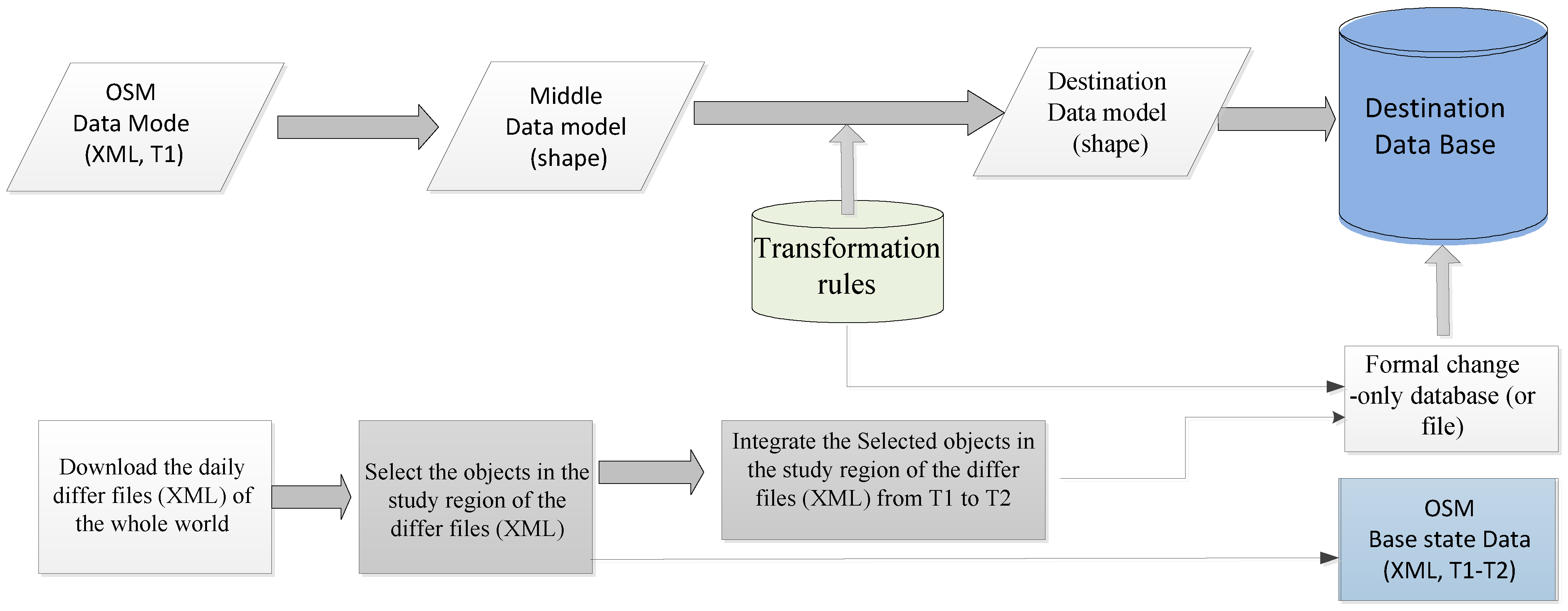
Based on the above analyses, we present a dynamic integration method for a borderland database using OSM data. In this method, the XML-formatted OSM data for a research borderland region are downloaded, and the primary and reference features are automatically converted into the shape-file-formatted middle data model (point, line, and area layers) according to OSM feature type definitions. A basic transformation rule base is formed by comparing the OSM-Map-Feature description document and the user data model definition file. Using these rules, the main features that comply with the OSM-Map-Feature definition can be automatically converted to the destination model. However, unusual features cannot be converted using the basic transformation rules. It is assumed that many unusual features are predominantly caused by different communication habits; in a special region, the volunteers usually have the same communication habit. Therefore, these unusual features can still be converted to the destination model using the rule-based method. Although it is difficult to form these rules from explicit knowledge, they can be formed using an automatic-remember mechanism during a human transformation process. Thus, this study develops both a human–computer interaction transformation model and a rules-machine-remember mechanism.

To keep the borderland database current, a method is developed to extract the change-only information for the research region from the global OSM daily diff file and to update the borderland database. In this method, the global daily diff file is downloaded automatically, and the changed objects in the given region are selected and stored in a database. The information (including spatial, semantic and change type) of the involved objects with multiple versions is integrated into a single version. Next, the change-only information database (or file) is produced using the designed format, and the change-only information is used to update the research borderland database automatically. This study’s strategy is shown in Figure 1.

Figure 1. The strategy for dynamically integrating a borderland database using OSM data.

Figure 1. The strategy for dynamically integrating a borderland database using OSM data.

4. The Rule-Based Model Transformation Method

As mentioned above, the OSM data model is usually different from the borderland research data model. In the OSM data model, node is the only primitive that contains coordinate information. Node includes the entity points and the coordinate points of way and relation objects. The nodes with tags are used to represent the point features, and the others are used to describe the locations of the ways and relations. A way is an ordered list of nodes. Simple ways (not close, not self-intersecting) are used to describe linear features, and closed ways represent simple area or circle line features. Relations are used to describe the topology, restriction, and complex regions (with holes). The key semantic information (“what is it” information) is described by tagging with key-value pairs in OSM XML. In the traditional GIS data models (e.g., ISO 14825, 2004, intelligent transportation systems-geographic data files, and the Chinese national fundamental geographic information system model), points, lines, and polygons (including simple and complex polygons) are represented directly; key semantic information (i.e., “what is it” information) is usually represented by codes; and objects with similar codes belong to the same layer. In the traditional GIS model, connective and adjacent relations are represented using a topological relationship table. The other relations represented in OSM (e.g., forward, backward, e-road_link, etc.) are usually stored in the attribute table. Furthermore, connective and adjacent relations can be generated automatically by many pieces of GIS software. Therefore, the aims of this study are related to model transformation and include the following tasks:

(1)

Extracting the point entities from nodes and converting them to the appropriate layer with codes in the destination model;

(2)

Determining whether the way objects are simple line, circle line, or simple polygon objects and assigning those objects to the corresponding layers using codes in the destination model;

(3)

Extracting the complex polygons from the relations and converting them to the appropriate layers using codes.

To achieve the above three aims, it is necessary to solve the following two problems. The first problem is to determine the spatial types of the objects, i.e., simple line, circle line, simple polygon, or complex polygon. The second problem is to convert objects to the appropriate layers using code.

As mentioned above, simple lines, circle lines and simple polygons are represented with ways. The open ways must be simple lines. The closed ways include circle lines and simple polygons. For example, a closed wall is still a line object (a trunk may be represented as a closed way object in OSM data) but in the borderland user database, a closed wall is usually represented as a line object. In these cases, the semantic information represented by “key-value” pairs is used to determine the spatial type of the closed ways. Complex polygons are objects with a k = “type” v = “multipolygon” tag and at least one role = the “inner” member and one role = the “outer” member in the relation. Using these properties, one can distinguish the complex polygons from the other relations.

Both the traditional GIS model and the OSM model share the convention that “all objects belong to a class and each object belongs to exactly one class”. According to this convention, one can construct a set of basic transformation rules using the official OSM-Map-Feature definition information and the user-data model definition information. Using these rules, the general objects can be converted to the appropriate layers (classes) in the destination model.

However, as mentioned in Section 3, many unusual features are tagged by neogeographers according to their communication habits, e.g., there are many features with “Key-value” pairs that are undefined in OSM formal map features. For example, the features tagged with “k = aeroway v = papi”, “K = waterway, V = spillway”, “papi” and “spillway” cannot be found in the OSM formal map features. These features have meaningful “key-value” pairs. Some other features do not have meaningful “key-value” pairs (e.g., features with “k = aeroway v = M?cQuy?”, “k = building v = yes”, “k = natural v = null”, etc.). 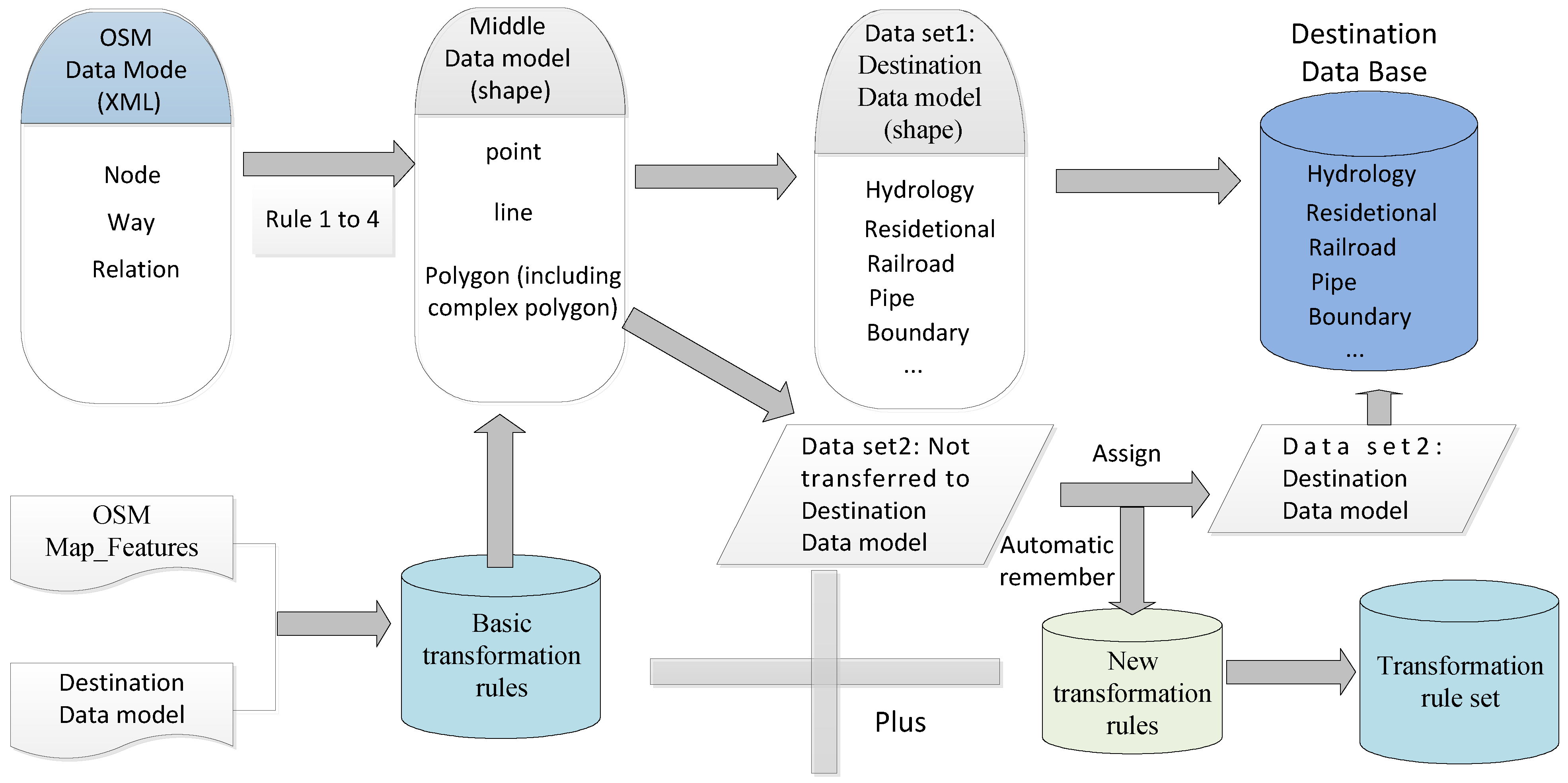For the first type of feature, i.e., the objects with a meaningful but undefined “key-value” pair, the value of “key” or “value” is not the suggested value defined in OSM-Map-Features and cannot be automatically converted to the user-appropriated layer (or classes) using basic rules. According to our analysis, many key-value pairs are shared within a special region in the OSM data. This phenomenon may be caused by different communication habits, but volunteers in the same region usually have the same communication habits. Therefore, the transformation can still be done using the rule-based method. The rules can be formed using an automatic-remember mechanism during a human transformation process. For example, when the editor assigns an appropriate code value to an unusual feature, the target layer of this unusual object will be determined automatically. Thus, not only the mapping relation between OSM key-value pairs and the target layer but also the target code will be remembered as a new rule that is stored in the rule base. Based on this observation, the strategy of the model transformation is shown in Figure 2.

The procedure for converting the OSM data into the destination data model includes the following steps:

Step 1: Determine the spatial type of the objects in the OSM data for the middle data model using the following spatial type transformation rules, i.e., Rules 1, 2, 3 and 4.

It is assumed that “OSMGeoPrim” denotes the geometric primitives (node, way and relation) in the OSM data and that “OSMtag.k” and “OSMtag.V” denote the semantic information key-value pairs in OSM XML. In traditional GIS, there is a convention that the boundary of an area object is closed. Therefore, in OSM data, the open ways are line objects (e.g., linear fence, road, open wall, etc.) and the area objects correspond to closed ways (e.g., a college campus, buildings, lakes, etc.). However, not all closed ways in OSM are area objects. According to our analysis, the following objects are usually presented as line objects in traditional 1:50000 spatial databases, i.e., the OSM features with “wall, busbar, fence, hedge, spikes, trunk_link, railway, footway, living_street, motorway, path, pedestrian, raceway, road, tertiary, track, breakwater, and pier” values. Therefore, using the geometric primitives and semantic properties, four spatial type transformation rules are developed using a 1:50000 spatial database as an example.

Figure 2. The model transformation strategy.

Figure 2. The model transformation strategy.

(1) A node with “Key-value” pairs is a point object.

Rule 1: If OSMGeoPrim = node && OSMtag.k ≠ Φ&& OSMtag.V ≠ Φ, then the node is a point object.

(2) An open way is a line object.

Rule 2: If OSMGeoPrim = way && Beginnode Equals Endnode = No, then the way is a line object.

(3) A closed way is usually an area object, except that the object has a “value” tag that equals one of the following: “wall, busbar, fence, hedge, spikes, trunk_link, railway, footway, living_street, motorway, path, pedestrian, raceway, road, tertiary, track, breakwater, or pier”.

Rule 3: If OSMGeoPrim = way && Beginnode Equals Endnode = Yes && (OSMtag.V ≠ wall, busbar, fence, hedge, spikes, trunk_link, railway, footway, living_street, motorway, path, pedestrian, raceway, road, tertiary, track, breakwater, or pier) then the way is a line object. Otherwise, the way is a simple polygon.

(4) A relation is a complex region if it has “k = type”, “V = multipolygon” values and at least one “Outer” and “Inner” polygon.

Rule 4: If OSMGeoPrim = relation && OSMtag.k = type && OSMtag.V = multipolygon && Number of “Outer” member ≥ 1 && Number of “Inner” member ≥ 1, then the relation is a complex region.

Therefore, using the above rules, the spatial type of the OSM objects can be determined automatically.

Step 2: Convert the general objects represented by the middle model to the appropriate layers with code in the destination model using the basic transformation rules.

Step 3: Interactively assign the unusual features that remain in the middle model (i.e., the dataset 2 in Figure 2) with the appropriate code and automatically determine which layers are suitable for them. Then, using the machine-remember mechanism, the assignments to the rule database are automatically remembered and the new-forming rules can be automatically used in the other data transformations.

It is assumed that “Mdl GeoPrim” denotes the geometric primitives in the middle data model and “Target Layer” and “Target code” denote the code and layer in the target model. Some example rules for converting the objects in the middle data model to the destination model are described in Table 1. The first rule in Table 1 can be interpreted as Rule 5.

(5) A point in the middle data model with “k = Natural Point” and “V = sea” corresponds to a point in “Hydrology Point layer” with “250000” code in the Chinese national fundamental geographic-information-data model.

Rule 5: If MdlGeoPrim = Point && OSMtag.k = Natural Point && OSMtag.V = sea, then TargetLayer = Hydrology Point, Targetcode = 250000.

Table 1. Exemplary rules for converting the spatial objects in the middle model to the user destination model.

Number	MdlGeoPrim	OSMtag.k	OSMtag.V	TargetLayer	Targetcode
1	Point	Natural Point	sea	Hydrology Point	250000
2	Point	Amenity Point	bus_station	Railroad Point	310300
3	Line	Building	wall	Residential Line	380201
4	Line	Highway	trunk	Railroad Line	430501
5	Polygon	Place	village	Residential Area	600100
6	Polygon	Waterway	river	Hydrology Area	210000

Note: In Table 1, a Chinese national fundamental geographic information data model is used as an example of a destination data model. In that model, the three types of geometric primitives belong to different layers.

Table 1. Exemplary rules for converting the spatial objects in the middle model to the user destination model.

Number	MdlGeoPrim	OSMtag.k	OSMtag.V	TargetLayer	Targetcode
1	Point	Natural Point	sea	Hydrology Point	250000
2	Point	Amenity Point	bus_station	Railroad Point	310300
3	Line	Building	wall	Residential Line	380201
4	Line	Highway	trunk	Railroad Line	430501
5	Polygon	Place	village	Residential Area	600100
6	Polygon	Waterway	river	Hydrology Area	210000

Note: In Table 1, a Chinese national fundamental geographic information data model is used as an example of a destination data model. In that model, the three types of geometric primitives belong to different layers.

Using the basic rules, the main features can be successfully converted to the destination model. However, because the unusual features are not defined in the OSM Map Feature document, they cannot be transferred using the basic rules. To solve this problem, a software tool was developed to interactively assign the unusual features to user classes with codes and to automatically remember this transfer knowledge as a rule. Thus, the rule base can be increased and the transformation power can be improved incrementally. Using this rule-based model transformation method, the OSM data can be converted to the user borderland data model.

5. Method for Extracting the Change-Only Information over a Period of Time

As mentioned above, borderland data must be updated incrementally. OSM data will remain as the low-cost, worldwide change-only information resource. However, in many borderland applications, the credibility and completeness of OSM data are insufficient and scientists must enhance the data quality and integrate other data sources to form a new data set. Usually, two methods are used for updating the user borderland database. One method is to convert the new OSM data directly using the model transformation method mentioned in Section 4 and then to check the converted data by cleaning or filtering the spurious or low-quality data and correcting the errors in it and integrating the other data sources each time. Because OSM data are collected by non-professional users without any specialized training, a large amount of spurious or low-quality data exists and a large amount of editing must be done before applying the data. This operation is difficult to do automatically (and such an undertaking lies outside the scope of this study). The interactive and repeated-editing processes are both error prone and labor intensive. Another method is to extract the change-only information from OsmChange and use it to update the integrated user borderland database. Because there is usually a much smaller amount of change-only data than existing data, if the change-only information extracting and updating process can be done automatically, a large amount of repeated editing will be avoided and efficiency is greatly improved. Therefore, the second method is more reasonable in our opinion.

OsmChange provides daily diff data for the entire world. Some companies (e.g., Geofabrik) provide daily diff data for many countries, e.g., Pakistan, Vietnam, etc. Such companies merely select the objects that change from the whole world daily diff to the country daily diff and do not provide complete information (e.g., spatial, semantic and change type) for the changed objects or methods for integrating the changed object information for a free-defined borderland region over a certain period. Furthermore, one object may be edited several times, and several versions with multiple change type values may exist in the diff files over a particular period. For updating, the information (including spatial, semantic and change type) in the multiple versions must be integrated into one version, especially the change type value that determines the updating operation and the value in the final version, which is usually not the real value. Therefore, extracting changed objects with complete information in the research region from OsmChange and determining the change-type value for the changed objects over a particular period are important issues when incrementally updating the borderland database.

5.1. Extracting the Objects in the Studied Region from the Diff Files

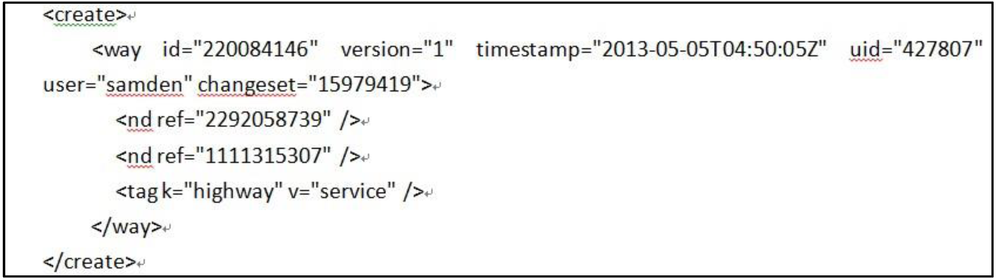
OsmChange provides a daily XML format diff file for the entire world. Because the daily diff files include change information for the entire world, the changed objects information in the studied region must be extracted from the world daily diff file. To determine whether the object is in the borderland region, each changed-object should have coordinates. Although they are similar to the OSM base state XML data, the spatial properties of the features are described as nodes, ways, and relations in the OSM diff file. In OSM diff files, there are three types of change sections: “modify”, “delete”, and “create” (we refer to “modify, delete, and create” as three change types in the following text). All of the objects belong to a single change section. These sections begin with “modify”, “delete”, and “create”, and end with “/modify”, “/delete”, and “/create”. The changed-objects information is located in the sections shown in Figure 3.

Figure 3. The OSM diff file format using the “create” way object section as an example.

Figure 3. The OSM diff file format using the “create” way object section as an example.

In OSM diff files, the changed nodes are located in the “/create”, “/modify”, and “/delete” node sections with complete coordinate information provided directly. One can extract the nodes in the research region using the point-in-polygon method of determination. In borderland analysis, sometimes the point on the boundary of the research region is an important node. For simplicity, this paper treats the nodes on the boundary of the research region the same as those that are within the research region. Therefore, it is easy to form a database of the changed node in the research region. This paper refers to this database as the ChgNodeInReg database.

The changed way and relation objects have only reference-nodes’ID in the corresponding sections, as shown in Figure 3. Furthermore, one can create a new way (or relation) object using the new nodes or the reference-nodes of the existing objects. However, the reference-nodes of the existing objects will not appear in the changed node sections even though they are the shape nodes of the new created objects. In addition, the reference-nodes of the existing objects will not appear in the ChgNodeInReg database. If the nodes are the existing objects in the research region, the coordinates have been stored in the local database. Otherwise, the coordinates must be downloaded from the OSM organization’s website. Therefore, there are several methods of obtaining the coordinates and determining whether they are in the research region for the changed way (or relation) objects. To extract the complete changed objects in the research region, we analyzed the topological relationships between the changed objects and the research region based on the topology thermos using the relation between simple line and region [29] as an example. The “delete” objects potentially appeared in the existing database or in former versions with coordinates. The Id of a “delete” object can be used to determine whether it is in the studied region. Therefore, we will mainly discuss the extraction method for “create” and “modify” objects in the text below.

From a topology perspective, the objects in the studied region are those objects that intersect the research region. Therefore, the relation between the simple way and research region is analyzed first. According to the topology theorem, there are seven basic relations between a simple line and a simple region, as shown in Figure 4. In Figure 4, R is the research region, C_m denotes the created objects, M_n denotes the modified objects, the red points denote the new or modified nodes, the black points denote the existing nodes, and W_i denotes the existing ways. The seven basic relations are “disjoint”, e.g., C₂, M₂, M₃ (in this diff file, M₃ is disjoint to R, although it may be changed from either an existing object that intersects R or a former created object during the former days in the period), “inside” (e.g., C₁, M₁), “touch at point” (e.g., C₄), “touch at line” (e.g., C₅), “on boundary” (e.g., C₇), “cross” (e.g., C₃ and C₆, M₄), and “Through” (e.g., C₈, C₉, M₅, and M₆).

After analyzing the component nodes of the changed ways that intersect with the research region, it was found that the component nodes can be divided into the following five cases:

(1)

New or modified nodes are in the research region (e.g., P₁, P₂, P₃, P₈, and P₉) denoted as ChgNodeInReg. The coordinates of these nodes can be picked in the downloaded daily diff.

(2)

New or modified nodes are not in ChgNodeInReg but comprise a reference node of the object that intersects the research region (e.g., P₄, denoted as ChgNodeNearReg). The coordinates of these nodes can also be picked in the downloaded daily diff.

(3)

The existing nodes are in the research region (e.g., P₅) that is denoted as ExsNodeInReg. The coordinates of these nodes can be chosen in the existing local database.

(4)

The existing nodes are not in the research region but comprise a reference node of the existing object that intersects the research region (e.g., P₇) denoted as ExsNodeNearReg. The coordinates of these nodes can also be picked in the local existing database.

(5)

Existing nodes are not in ExsNodeInReg and ExsNodeNearReg, e.g., P₆, which is denoted as ExsNodeOutReg. The coordinates of these additional nodes need to be downloaded from OSM’s official website.

Figure 4. The relationships between changed way and the research region considering the evolution of the objects.

Figure 4. The relationships between changed way and the research region considering the evolution of the objects.

Therefore, the spatial information (i.e., the coordinates of the component nodes) of all of the objects in the daily diff files can be obtained in one of these five ways.

As mentioned above, the changed objects in the studied region are the objects that intersect the research region, e.g., C₁, C₃, C₄, C₅, C₆, C₇, C₈, C₉, M₁, M₄, M₅, and M₆ (Figure 4). After further analysis, it can be concluded that the objects with one or several nodes in the studied region (e.g., C₁, C₃, C₄, C₅, C₆, C₇, C₉, M₁, M₄, M₆ in Figure 4) are the objects that should be reserved. Not all objects without a node in the studied region are disjointed from the research region (e.g., C₈ and M_5. C₈ and M₅ are objects that intersect R but do not have a node in R). In addition, the modified objects are disjointed from the research region in a daily diff file, and if the object has a corresponding existing object or at least one former version that intersects the studied region (e.g., M₃), it will still be reserved. Therefore, five rules can be concluded for extracting objects in the studied region from the diff files.

It is assumed that “NodeInWay” denotes the node set of the changed way; “IsWayIntertsectR” is a function used to determine whether the way intersects the studied region; “WayId” is the ID of the way; “BaseNodeInReg” and “BaseWayInReg” denote the existing nodes (or ways) in the studied region; “ChgNodeInReg” and “ChgWayInReg” denote the changed nodes (or ways) in the studied region; and “ChangeType” ChangeType is a variable used to store the change section begin-flag (“modify”, “delete”, “create”).

(1) If a way with one node in the node set of the changed way is in the existing nodes set or the changed nodes set; the way is a changed way in the studied region.

Rule 1: If NodeInWay ∩ (BaseNodeInReg∪ChgNodeInReg) ≠ Φ, then the way is stored to ChgWayInReg.

(2) If a way is without a node in the existing nodes set or the changed nodes set but the way intersects the research region, the way is still a changed way in the studied region.

Rule 2: If NodeInWay ∩ (BaseNodeInReg∪ChgNodeInReg) = null, and IsWayIntertsectR = true, then stored it to ChgWayInReg.

(3) If a way is without a node in the existing nodes set or the changed nodes set, the way has no intersection with the research region and the ChangeType is “create”, the way is a changed way outside the scope of the studied region and it can be discarded

Rule 3: If NodeInWay ∩ (BaseNodeInReg∪ChgNodeInReg) = null, IsWayIntertsectR = false, and the “changetype” = “create”, then discard the way.

(4) If a way is without a node in the existing nodes set or the changed nodes set and the way has no intersection with the research region but the ChangeType is “modify” and the ID of the way is in the existing (or changed) ways in the studied region, the way has at least one former version that intersects the studied region and should be stored to ChgWayInReg with a flag to show that it is disjointed from the research region.

Rule 4: If NodeInWay ∩ (BaseNodeInReg∪ChgNodeInReg) = null, IsWayIntertsectR = false, the “ChangeType” = “modify”, and WayId ∩ (BaseWayInReg∪ChgWayInReg) ≠ Φ, then store it to ChgWayInReg with a disjoint flag.

(5) If a way is without a node in the existing nodes set or the changed nodes set, the way has no intersection with the research region, the ChangeType is “modify”. If the ID of the way is not in the existing (or changed) ways in the studied region, then all former versions of the way (including the way itself) are disjointed from the research region and should be discarded.

Rule 5: If NodeInWay ∩ (BaseNodeInReg∪ChgNodeInReg) = null, IsWayIntertsectR = false, the “ChangeType” = “modify”, and WayId ∩ (BaseWayInReg∪ChgWayInReg) = null, then discard it.

Therefore, using the above methods and rules, the changed nodes and ways in the research region can be automatically extracted with complete information. For the complex polygons in relations, if the outer polygon is a polygon that intersects the studied region, the complex polygon is an object that intersects the research region and should be stored. The outer polygon is also a simple way and, therefore, the complex polygons in relations can also be extracted using the above methods and rules.

5.2. Integrating the Selected Changed Objects over a Period of Time

As mentioned above, there are usually several versions for one object in the selected object set over a period. Each version has its change type and semantic information with the same ID. If the last version is used to update the existing data it may cause the updating process to be done incorrectly. For example, where one object has three versions in the set, the change types are “create”, “modify”, and “delete”, respectively. If the last version with the “delete” change type is used to update the existing data (because this object is not included in the existing data base), a wrong will be reported by the updating agent. Indeed, this object is invalid and should not be included in the change-only information file. Therefore, a method is needed to determine the change-type of the multi-edition objects over time.

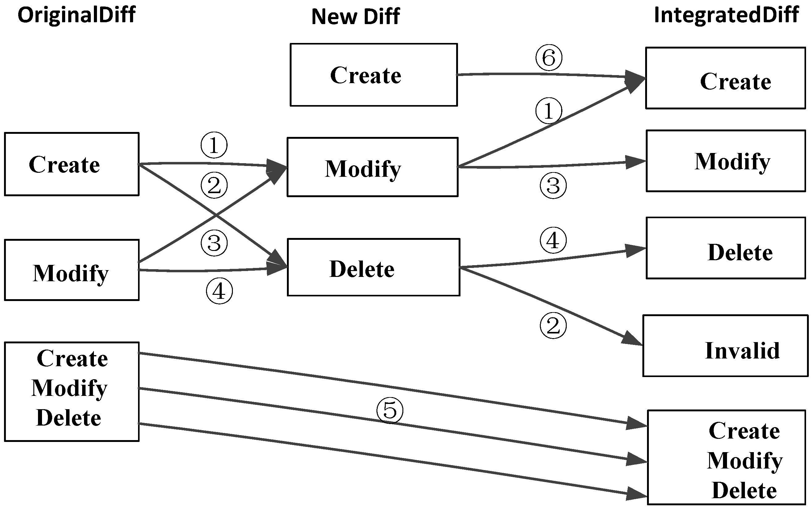
Because the multi-version objects have been edited several times in sequence, the integrating process should be made according to the time sequence. After analyzing the evolution of the changed objects involving the neighbor diff files, six types of change-type evolution are identified for the involved objects between the neighbor diff files. It is assumed that “original diff” is a diff file used to store the integrated changed objects (the first original diff file for the period of time is the first daily diff file), “New diff” is the next day diff file of the “original diff”, and “Integrated diff” is the result diff file. The change-type evolution of objects is shown in Figure 4.

In Figure 5, the six types of change-type evolution are listed as follows:

(1)

If the change-type of the object is “create” in the original diff file and “modify” in the new diff file, then the object is a “create” object in the integrated diff file;

(2)

If the change-type of the object is “create” in the original diff file and “delete” in the new diff file, then the object is a “invalid” object and will not be included in the integrated diff file;

(3)

If the change-type of the object is “modify” in the original diff file and “modify” in the new diff file, then the object is a “modify” object in the integrated diff file;

(4)

If the change-type of the object is “modify” in the original diff file and “delete” in the new diff file, then the object is a “delete” object in the integrated diff file;

(5)

If the changed object (the change-type includes “create”, “modify”, or “delete”) is in the original diff file and it does not appear in the new diff file, then the object is in the integrated diff file remained the same change-type value;

(6)

If the object first appears in the new diff file and its change-type is “create”, then the object is a “create” object in the integrated diff file.

Figure 5. Change-type evolution of the objects between the neighbor versions.

Figure 5. Change-type evolution of the objects between the neighbor versions.

Based on the above analysis of the change-type evolution of the objects between the neighbor versions and the object-extracting process, especially for the evolution of the modified objects, seven rules are determined for integrating the changed objects. It is assumed that “ChgObjectInReg” is the selected changed-object database over the period of time, V₁ and V_max (max ≥ 1) are the first and last version of an object in “ChgObjectInReg”; and ChangeTypeV₁, ChangeTypeV_max and ChangeTypeO denote the ChangeType of V₁, V_max and the integrated object, respectively.

(1) If the object first appeared in the new diff file and the ChangeType of the integrated object equals that of the first version it is usually a “create” object.

Rule 1: if max = 1, then ChangeTypeO = ChangeTypeV₁ it is stored to ChgObjectInReg.

(2) If the object is created in the former version, modified in the next version, and disjointed from the research region (with a “disjoint” flag) in the final version, it should be discarded.

Rule 2: if max ≥ 1, ChangeTypeV₁ = “create”, and ChangeTypeV_max = “modify”, and the last version with a “disjoint” flag (Section 5.1), then discard it.

(3) If an object is created in the former version, modified in the next version, and not disjointed from the research region (without a “disjoint” flag) in the final version, then the object is created during the period and should be stored.

Rule 3: if max ≥ 1, ChangeTypeV₁ = “create”, and ChangeTypeV_max = “modify”, and the last version without “disjoint” flag (Section 5.1), then ChangeTypeO = “create”, it is stored to ChgObjectInReg.

(4) If an object is created in the former version, and “delete”in the next version, then it is an “invalid”object, and it should be discarded.

Rule 4: if max ≥ 1, ChangeTypeV₁ = “create”, and ChangeTypeV_max = “delete”, then discard it.

(5) If the change type of an object is “modify” in the former version, “modify” in the next version, and disjointed from the research region (with a “disjoint” flag) in the final version, then the object is contracted to disjoint from the research region and it should be deleted from the integrated diff file.

Rule 5: if max ≥ 1, ChangeTypeV₁ = “modify”, and ChangeTypeV_max = “modify”, and the last version with a “disjoint” flag (Section 5.1), then ChangeTypeO = “delete”, it is stored to ChgObjectInReg with removed reason flag “contraction”.

(6) If the change type of an object is “modify” in the former version, “modify” in the next version, and not disjointed from the research region (without a “disjoint” flag) in the final version, then the object is modified during the period and should be stored.

Rule 6: if max ≥ 1, ChangeTypeV₁ = “modify”, and ChangeTypeV_max = “modify”, and the last version without “disjoint” flag (Section 5.1), then ChangeTypeO = “modify”, it is stored to ChgObjectInReg.

(7) If the change type of an object is “modify” in the former version, and “delete” in the next version, then the object is a “delete” object during the period.

Rule 7: if max ≥ 1, ChangeTypeV₁ = “modify”, and ChangeTypeV_max = “delete”, then ChangeTypeO = “delete”, it is stored to ChgObjectInReg.

It is assumed that the spatial and thematic information of the last version is the best, and the information in the last version is used as the integrated object. Therefore, using the above rules, the changed objects with multi-versions can be integrated into one version to produce a change-only information file (or database) automatically. With the change-only file, both the user destination database and the research region OSM XML state file can be updated by automatically eliminating the deletion objects, replacing the modified objects, and creating the new objects [30].

6. Experimental Application

Based on the rules and algorithms mentioned above, we enabled the automatic (or semiautomatic) integration and updated the borderland database by programming with Visual C# 2010. The developed system was intensively tested using a Chinese national fundamental geographic information data model as the user model and extending the name from the Chinese name to include both the English name and the mother language name. In this experiment, the tag “HydA” denotes “Hydrological Area”, “Hydl” denotes “Hydrological Line”, “HydFacA” denotes “Hydrological Facility Area”, “ResiA” denotes “Residential Area”, “ResiFacP” denotes “Residential Facility Points”, “ResiFacA” denotes “Residential Facility Area”, “BouP” denotes “Boundary Point”, “VegA” denotes “Vegetable Area”; “TerP” denotes “Terrain Point”, “TraP” denotes “Traffic Point”, and “WatA” denotes “Water Area”.

6.1. Model Conversion Experiment

In this experiment, the OSM Vietnam data from 8 October 2013 is converted to the Chinese national fundamental data model using Rule set 1 (the 1180 basic rules). The remaining objects are converted to the user model using the interactive software tool, and 160 more rules are stored automatically to form Rule set 2, as shown in Figure 6 (in Figure 6, the lower picture provides details of the red box in the upper picture). The OSM Pakistan data from 16 October 2013 is converted to the Chinese national fundamental data model using Rule set 1, which uses the 1180 basic rules, and Rule set 2 (i.e., 1180 basic rules plus the 160 additional rules generated in the interactive assignment in the Vietnam experiment), respectively. Overall, 109855 features are transferred by Rule set 1, and 1801 additional objects are transferred by Rule set 2. However, 398 remaining objects could not be transferred by these rules. Using the interactive software tool, the remaining objects are converted to the user model and 224 more rules are stored automatically.

Figure 6. Model transformation experiment data (Vietnam, 8 October 2013). (a) The data transferred by the 1180 basic rules; (b) the objects cannot be transferred using the basic rules; (c) the complete data can be transferred using universal rules.

Figure 6. Model transformation experiment data (Vietnam, 8 October 2013). (a) The data transferred by the 1180 basic rules; (b) the objects cannot be transferred using the basic rules; (c) the complete data can be transferred using universal rules.

Detailed information on the main layers using the different rule sets is shown in Table 2. To test the correctness of the model conversion, all of the converted features of Islamabad in Pakistan and Qui Nhon in Vietnam are used for comparison with corresponding Google images. The comparison result is shown in Table 3.

Table 2. Features converted by different rule set.

TargetLayer	Vietnam Data			Pakistan Data
	Ftr1	Ftr2	Increase (%, 2-1)	Ftr1	Ftr2	Ftr3	Increase (%, 2-1)	Increase (%, 3-1)	Increase (%, 3-2)
HydA	2775	2813	1.4	1047	1076	1077	2.7	2.7	0.1
HydFacA	1994	3073	35.1	601	1476	1506	59.3	60.1	2.0
ResiFacP	8337	8460	1.4	3380	3433	3561	1.5	5.1	3.6
ResidA	3076	3174	3.1	3304	3404	3434	2.9	3.8	0.9
TraL	79969	79978	0	77954	77954	77971	0	0	0
BouP	2594	2600	0.2	4262	4268	4341	0.1	1.8	1.7
TerA	59	80	26.2	294	307	330	4.2	10.9	7.0
VegA	764	1064	28.2	434	727	760	40.3	42.9	4.3
The others	99568	101242	1.6	91276	92645	92980	1.5	1.8	0.3
Total	112036	114496	2.1	109855	111656	112054	1.6	2.0	0.3

Notes: In Table 2, Ftr1, Ftr2 and Ftr3 denote that the features converted by the basic rule database, Rule base 2, and Rule base 3, respectively; “increase (%, 2-1)” denotes the increased ratio of the transformation features, and “2-1” means that (Ftr2 − Ftr1) / Ftr2.

Table 2. Features converted by different rule set.

TargetLayer	Vietnam Data			Pakistan Data
	Ftr1	Ftr2	Increase (%, 2-1)	Ftr1	Ftr2	Ftr3	Increase (%, 2-1)	Increase (%, 3-1)	Increase (%, 3-2)
HydA	2775	2813	1.4	1047	1076	1077	2.7	2.7	0.1
HydFacA	1994	3073	35.1	601	1476	1506	59.3	60.1	2.0
ResiFacP	8337	8460	1.4	3380	3433	3561	1.5	5.1	3.6
ResidA	3076	3174	3.1	3304	3404	3434	2.9	3.8	0.9
TraL	79969	79978	0	77954	77954	77971	0	0	0
BouP	2594	2600	0.2	4262	4268	4341	0.1	1.8	1.7
TerA	59	80	26.2	294	307	330	4.2	10.9	7.0
VegA	764	1064	28.2	434	727	760	40.3	42.9	4.3
The others	99568	101242	1.6	91276	92645	92980	1.5	1.8	0.3
Total	112036	114496	2.1	109855	111656	112054	1.6	2.0	0.3

Notes: In Table 2, Ftr1, Ftr2 and Ftr3 denote that the features converted by the basic rule database, Rule base 2, and Rule base 3, respectively; “increase (%, 2-1)” denotes the increased ratio of the transformation features, and “2-1” means that (Ftr2 − Ftr1) / Ftr2.

Table 3. Sum of model conversion error.

Layer Name	Features		Conversion Error Features		Conversion Error Percentage
	Islamabad	Qui Nhon	Islamabad	Qui Nhon	Islamabad	Qui Nhon
HydA	6	16	1	2	16.7%	12.5%
Hydl	39	9	0	1	0	11.1%
Resi-A	73	15	0	0	0	0
ResifacA	268	84	5	11	1.9%	13.0%
ResifacP	528	57	0	0	0	0
TraL	4038	687	0	0	0	0
BouP	38	9	2	0	5.2%	0
VegA	39	37	3	3	7.7%	8.1%
Sum of single city	5029	914	11	17	0.2%	1.9%
Total of two cities	5943		28		0.5%

Table 3. Sum of model conversion error.

Layer Name	Features		Conversion Error Features		Conversion Error Percentage
	Islamabad	Qui Nhon	Islamabad	Qui Nhon	Islamabad	Qui Nhon
HydA	6	16	1	2	16.7%	12.5%
Hydl	39	9	0	1	0	11.1%
Resi-A	73	15	0	0	0	0
ResifacA	268	84	5	11	1.9%	13.0%
ResifacP	528	57	0	0	0	0
TraL	4038	687	0	0	0	0
BouP	38	9	2	0	5.2%	0
VegA	39	37	3	3	7.7%	8.1%
Sum of single city	5029	914	11	17	0.2%	1.9%
Total of two cities	5943		28		0.5%

The experiment shows that the model-conversion rule-remember mechanism can increase the rule base incrementally and efficiently improve the model’s transformation power. The total conversion error percentage of the two cities is 0.5%. This demonstrates that the conversion accuracy is reasonable. After analysis of the error conversion features, we found that the reason for conversion error was primarily caused by the volunteers’ different types of notations.

6.2. Updating Experiment

In the updating experiment, Pakistan data converted from OSM for 30 November 2014, is used as the base state, and the OSM differ data are from 30 November 2014 to 30 January 2015, as the change-only information source data for Pakistan. Overall, 10,657 objects are created, 7070 objects are modified, and 587 objects are deleted. The experimental data is shown in Figure 7, and the underside picture with imagery is the details of the red box in the upper side picture. The distribution of the objects is shown in Table 4.

Figure 7. The incremental updating experiment using OsmChange data. (a) The Pakistan data converted from OSM for 30 November 2014; (b) the change-only data from 30 November 2014 to 30 January 2015; (c) the updated data of Pakistan at 30 January 2015.

Figure 7. The incremental updating experiment using OsmChange data. (a) The Pakistan data converted from OSM for 30 November 2014; (b) the change-only data from 30 November 2014 to 30 January 2015; (c) the updated data of Pakistan at 30 January 2015.

Table 4. The distribution of the objects in the updating experiment

Layer Name (Type)	OSM Download Data (30 November)	Updated Data (30 January)	OSM Download Data (30 January)	Created Objects	Modified Objects	Deleted Objects
BouP	7930	8004	8004	84	83	10
PipeP	11894	11907	11907	19	1	6
ResiP	5279	5588	5588	341	98	32
TerP	184	190	190	6	1	0
TraP	2796	2901	2901	137	100	32
WatP	1249	1254	1254	8	0	3
BouL	246	246	246	0	4	0
PipeL	429	430	430	1	1	0
ResiL	2567	2589	2589	25	4	3
TerL	49	49	49	0	0	0
TraL	114325	123172	123172	9265	6445	418
VegL	6	6	6	0	0	0
WatL	7183	7312	7312	146	99	17
BouA	573	573	573	24	3	4
ResiA	19918	20416	20416	553	173	55
TerA	281	283	283	3	1	1
VegA	1183	1206	1206	28	18	5
WatA	3578	3612	3612	35	39	1
Sum	179670	189758	189758	10675	7070	587

Table 4. The distribution of the objects in the updating experiment

Layer Name (Type)	OSM Download Data (30 November)	Updated Data (30 January)	OSM Download Data (30 January)	Created Objects	Modified Objects	Deleted Objects
BouP	7930	8004	8004	84	83	10
PipeP	11894	11907	11907	19	1	6
ResiP	5279	5588	5588	341	98	32
TerP	184	190	190	6	1	0
TraP	2796	2901	2901	137	100	32
WatP	1249	1254	1254	8	0	3
BouL	246	246	246	0	4	0
PipeL	429	430	430	1	1	0
ResiL	2567	2589	2589	25	4	3
TerL	49	49	49	0	0	0
TraL	114325	123172	123172	9265	6445	418
VegL	6	6	6	0	0	0
WatL	7183	7312	7312	146	99	17
BouA	573	573	573	24	3	4
ResiA	19918	20416	20416	553	173	55
TerA	281	283	283	3	1	1
VegA	1183	1206	1206	28	18	5
WatA	3578	3612	3612	35	39	1
Sum	179670	189758	189758	10675	7070	587

The experiment shows that the downloaded OSM data are equal to the data updated from the OsmChange daily diff file; therefore, using the OsmChange daily diff file to create the change-only information of the research region is a reasonable method of updating the borderland database.

7. Conclusions and Discussion

In this article, we present a dynamic integration method for borderland databases using OSM data. In this method, the XML-formatted OSM data for a research borderland region are downloaded, the spatial types of the objects in OSM data are determined using spatial type transformation rules, and the data are converted to the middle data model. A basic transformation rule base is formed by comparing the OSM Map Feature description document and the destination model definitions; using the basic rules, the main features can be automatically converted to the destination model. A human-computer interaction model transformation and an automatic rule-remember mechanism are developed to interactively transfer the unusual features that cannot be transferred by the basic rules to the suitable target layers and to remember the reusable rules automatically. To keep the borderland database current, the global OsmChange daily diff file is used to select the change-only information of the research region. To select the changed objects in the region under study, the relationship between the changed object and the research region considering the evolution of the involved objects is analyzed, five rules used to select the objects are concluded. To integrate the changed objects with the multi-version over a given period time, the change-type evolution of the objects with multi-version is analyzed and seven rules are formulated to determine the change-type of the objects with multi-versions.

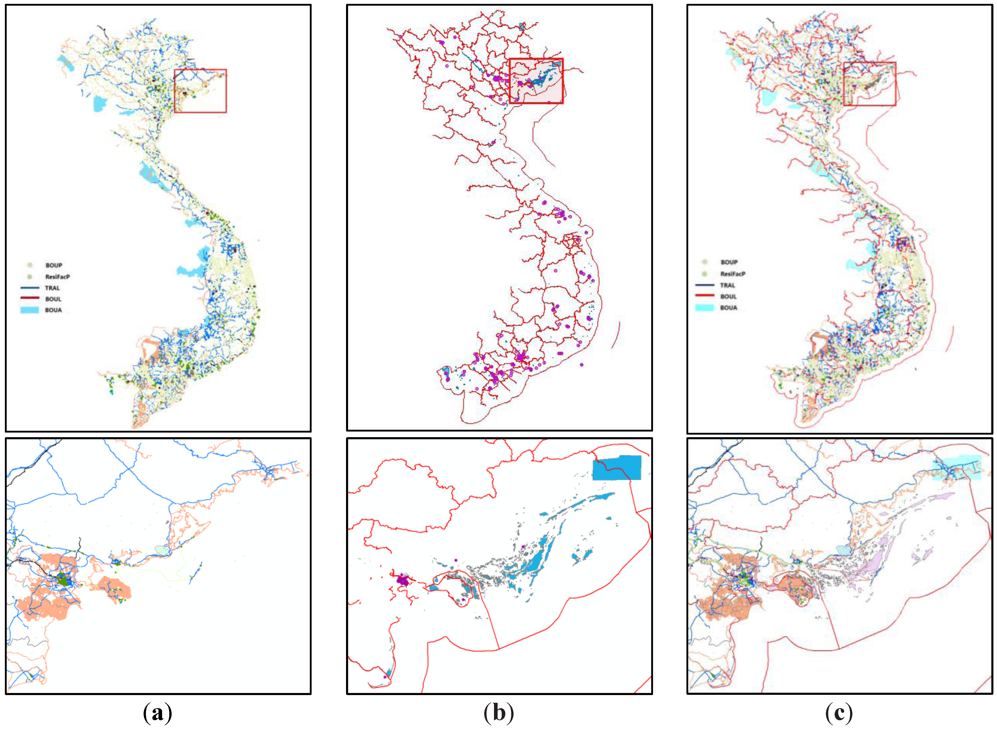
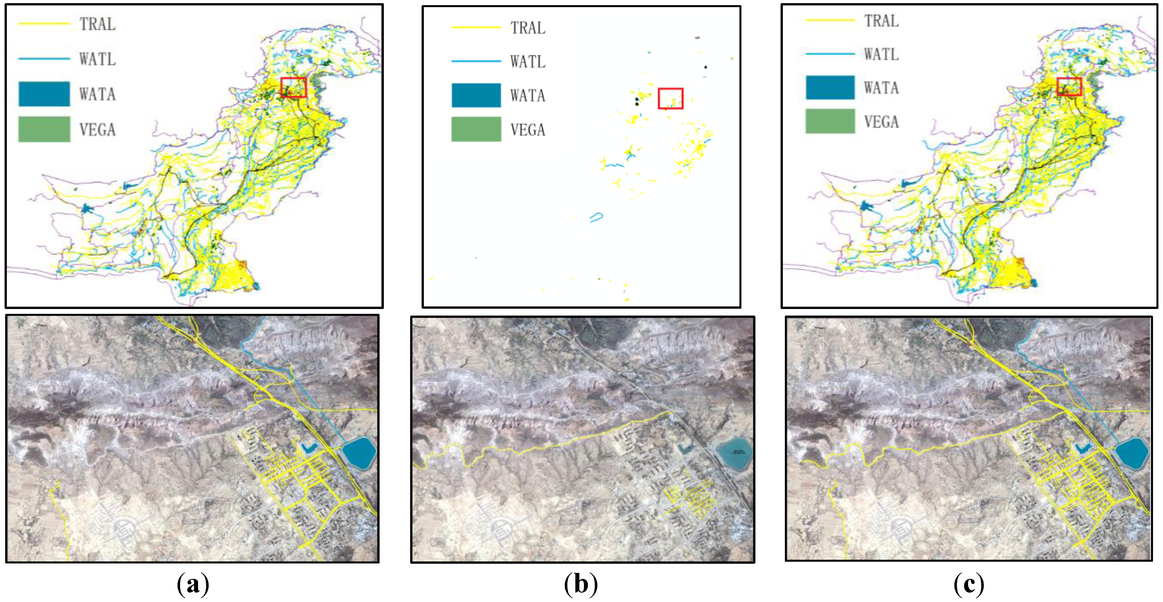
To test the correctness of the methods and algorithms presented in this paper, a prototype system is developed by programming with Visual C# 2010. The developed system was intensively tested using the Chinese borderland fundamental geographic information data model as the destination user model and the OSM data for Vietnam and Pakistan as experimental data. The experiment showed that the rule-remember mechanism could both increase the rule base incrementally and improve the model transformation power efficiently. Moreover, its conversion accuracy is reasonable, and the data updated using the updating method presented in this paper are equal to the newly downloaded OSM data.

From the above research experience, a dynamic integration method using OSM data is achieved. Although this method is developed to integrate and update the borderland database using OSM data, the method and algorithms can also be used to integrate and update other user databases. A primary model transformation rule base from OSM data to a 1:50,000 Chinese borderland fundamental geographic information data model has been formed. This rule base has 1180 basic rules and 1164 additional automatic remembered rules. An elementary 1:50,000 Chinese borderland geographic information database has been created at a very low cost. Some lessons can also be learned from the research experience. (1) In forming model transformation rules, this research uses only the tag values in the key and value columns to construct the basic rule database. Indeed, many refinement features described in the comment column are used as the tagging value in OSM data. Therefore, the refinement features in the comment can be used to construct the model transformation rule database. (2) In our early research for extracting the changed objects in the studied region, the complete relationships between the changed way and the research region are not analyzed, and only the ways with nodes in the research region are extracted, which caused some ways (without nodes in the research region, but with intersection to the research region) to be missed. (3) Because the change-type evolution of the objects between the neighbor versions were not noted at first, some objects with “modify” change type in the former version, “modify” in the next version, and disjointed from the research region in the last version remained in the updated database. Therefore, the result is inconsistent with the downloaded OSM data.

It is necessary to state that some features in the OSM data lack valid “key-value” properties that still cannot be automatically converted to the destination model using the rule-based method presented in this paper. Additionally, this paper assumes that the spatial and thematic information of the last version is the best and that the information in the last version is used as the integrated object. Although OSM data is voluntarily produced by amateurs (‘neogeographers’), the last version may not be the best version. The credibility of the volunteers affects OSM data quality, and future work will focus on integrating the change objects with the multi-version considering the object’s reliability.