Bridge Performance Assessment Based on an Adaptive Neuro-Fuzzy Inference System with Wavelet Filter for the GPS Measurements

Abstract

This study describes the performance assessment of the Huangpu Bridge in Guangzhou, China based on long-term monitoring in real-time by the kinematic global positioning system (RTK-GPS) technique. Wavelet transformde-noising is applied to filter the GPS measurements, while the adaptive neuro-fuzzy inference system (ANFIS) time series output-only model is used to predict the deformations of GPS-bridge monitoring points. In addition, GPS and accelerometer monitoring systems are used to evaluate the bridge oscillation performance. The conclusions drawn from investigating the numerical results show that: (1)the wavelet de-noising of the GPS measurements of the different recording points on the bridge is a suitable tool to efficiently eliminate the signal noise and extract the different deformation components such as: semi-static and dynamic displacements; (2) the ANFIS method with two multi-input single output model is revealed to powerfully predict GPS movement measurements and assess the bridge deformations; and (3) The installed structural health monitoring system and the applied ANFIS movement prediction performance model are solely sufficient to assure bridge safety based on the analyses of the different filtered movement components.

1. Introduction

Long-span bridges are crucial links between cities and countries. For this reason, it is important to investigate the performance of bridge components. Structural health monitoring (SHM) systems are good tools for such investigations [1,2]. There are short-term and long-term SHM systems [1,2,3]. For the assessment of the oscillations of a long-span bridge, it is better to use the long-term monitoring system for the bridge members, and to study the behavior of the bridge to assess the safety level throughout its life. Liu et al. [4] have concluded the objectives of bridge monitoring systems. Moreover, the deformations of critical structures, such as bridges, are also required to be assessed from the economic viewpoint.

Over the last decade, SHM has become an increasingly accepted technology for the prognosis of the condition and safety of bridges [2,4,5]. The continuously-measured position data from an online SHM system is used to estimate the status of deformation, which is among the most critical forms of damage which can occur in a long-span bridge.

The global positioning system (GPS) is widely employed to measure deformation applications, such as for smart structures. GPS receivers have been applied as universal time and frequency standards [6]. Along with the development of GPS software, hardware, and sampling rate improvement of the GPS receiver, GPS has shown remarkable superiority in monitoring the dynamic deformations of large structures with high accuracy. The advancements of GPS measurement with a real-time kinematic (RTK) system are discussed by Yu et al. [7]. GPS observations are often corrupted by noise and errors, which may severely limit their usefulness [8,9,10]. Moreover, the noise characteristics of records describing the dynamic vibrations affect the GPS measurements [6,8]. The types of GPS errors and de-noising of GPS measurements have been clearly described in [9].

The filtration or smoothing of GPS measurements is important and is applied before analyzing the GPS monitoring data, in order to remove errors and extract the information needed in order to calculate correctly the deformation of a structure. Many types of filters and smoothes are used to extract the components of structural movement [6,7,8,10]. Nowadays, the wavelet transform (WT) is a powerful tool in signal processing [9,11,12,13]. Signal de-noising is a topic that continually draws great interest. Therefore, in this study, we will apply the wavelet transform de-noising to improve the GPS measurements.

In reality, real-time measurement signals are non-stationary and their frequency changes have been divided into slow change and quick change. The smoothing filters in GPS are partitioned into two groups: position domain filters and range domain filters. Position domain filtering always shows better performance than range domain filtering [9]. Moreover, Mosavi and Gholipour [9] have found that the WT can effectively improve the single frequency GPS positioning precision. In addition, Postalcloglu et al. [14] have studied the comparison between WT and Kalman filter for the time series noisy signal data. They have found that WT is suitable for mitigating noises and errors in the time series signal. Many studies have used WT to remove the noises and errors from GPS measurements [8,9,11,13,15].

Investigating the movements and deformations of bridges plays a crucial rule in bridge safety assessment through examining the bridges performance and predicting their safety in the future. Previously, many methods were used to predict the nonlinear GPS measurements. One of these methods is the Kalman filter solution, which is represented as a random process. The Kalman filter is expressed using stochastic models [16]; such models include the first or higher order Gauss-Markov model [17] and auto-regressive models [18]. These models provide only an approximate description of movement behavior.

On the other hand, artificial neural networks (ANN) have been widely used to predict the behavior of structures and to mitigate GPS errors [18,19,20,21]. The adaptive neuro-fuzzy inference system (ANFIS) depends on ANN. In addition, it uses the Takagi-Sugeno (TS) fuzzy inference system (FIS), TS-FIS, to define the parameters model [22]. Iphar [23] has compared different dynamic prediction models for ANN and ANFIS, finding that ANFIS is the more accurate model in predicting dynamic measurements. Time series ANFIS predicting models have received wide attention among researchers in the last few decades [22,24]. The advantage of ANFIS theory is its ability to deal with time series data rather than the crisp point data which is used to describe GPS movement errors [16]. The Kalman and ANFIS models with Kalman model prediction deferential GPS (DGPS) were compared in Abdel-Hamid et al. [16]. It was found that the ANFIS model has the ability to reimburse the absence of updated DGPS measurements and maintain consistent positioning accuracy.

The main objective of the present study is to design an ANFIS model for the GPS-bridge movement assessment. The study aims to demonstrate the use of the wavelet transform de-noising method in removing the GPS measurement noises, and to study the availability of this method for long-term GPS monitoring data. It also investigates the accuracy of the ANFIS prediction model in measuring bridge performance. To do this, the study focuses on assessing the behavior of the Huangpu Bridge based on SHM and the designed prediction model.

2. Bridge Structural Health Monitoring System

The Huangpu road bridge, opened in 2008, was the key project on the second ring highway in Guangzhou, China. Details about the bridge design and its structural characteristics can be found in Wang et al. [25].The bridge connects the Central Business District of Guangzhou and Panyu District (Figure 1). It crosses the Pearl River between the Guangzhou Overseas Ship Maintenance Plant and the Boluomiao Shipyard. The bridge is a combined suspension and cable-stayed bridge. Its total length is 7049 m. The suspension bridge portion has a main span of 1108 m and the cable-stayed portion spans 383 m (Figure 2). The total width of the deck is 41.00 m and the height of the towers is 226.14 m.

A long-term SHM system has been designed and implemented on the bridge to monitor its performance (Figure 2). The system includes twenty-two uniaxial accelerometers, which were permanently installed on the deck to measure the vertical and horizontal vibrations. Ten GPS units were installed to monitor the bridge deck movements in three directions (Figure 2). Three extra GPS units and three extra uniaxial accelerometers were installed to monitor the towers’ movements and vibrations in two directions (Figure 2).

Figure 1. Huangpu bridge view.

Figure 1. Huangpu bridge view.

Figure 2. Bridge elevation and health monitoring system.

Figure 2. Bridge elevation and health monitoring system.

The collected GPS data were resolved from rover stations, and the base station was fixed near the bridge. The bridge movement points are represented relative to the base station point. A local bridge coordinate system (BCS) was chosen for the observation analysis and evaluation. In this case, the X, Y, and Z axes indicate the bridge traffic and the lateral and vertical directions, respectively. This coordinate system is assumed to bebeneficial for observation, evaluation, and description of the bridge’s deformation. It also allows a better interpretation of the analysis results as they relate to the deformation directions. Leica antenna double-frequency GPS receivers were used. The satellite elevation cut-off angle is 13^°with at least nine satellite views. The reference station refreshes the RTK correction messages for the GPS monitoring stations with one Hzsampling frequency in each direction. Due to the large data files, the sessions are split into single-day measurements for processing purposes. The collected data are mixed with that generated by the receiver’s own oscillators, and then processed using Spider 2.1 RTK software. More details can be found at Kaloop and Kim [26].

3. Wavelet Transform De-Noising of the GPS Measurements

The wavelet transform (WT) is a signal processing tool which has been developed over the last decade. WT is very suitable for non-stationary signals such as the separation of signal and noise because of its availability for evaluation of the time and frequency domains. It also has good localization properties and multi-resolution analysis in the characteristic measurements of sensors. The WT method is described in more detail by Xizheng et al. [13]. The continuous wavelet transform must be discrete in practice, especially when implemented on a computer [13]. Therefore, in this study, the discrete wavelet transform (DWT) type is applied. The WT for the signal f(t) can be considering as follows, from Xizheng et al. [13]:

$${\text{WT}}_{\text{f}}\text{ (a,b)}=\text{(f},{\text{φ}}_{\text{a,b}}\text{)}$$

(1)

Where ${\text{φ}}_{\text{a},\text{b}}$ (t) is the continuous wavelet at time (t) can be presented as follows:

$${\text{φ}}_{\text{a,b}}{\text{ (t)=|a|}}^{\text{(-1/2)}}\text{ φ( (t-b)/a)}$$

(2)

Where a and b are the scale parameter and transition parameter, respectively. In addition, the discretization is towards continuous scale parameter and continuous translation parameter, but not time parameter. In this case $\text{b}\in \text{R, a}\in R^{+},a\ne 0$ and φ is allowed, for convenience, a must be limited to positive in discretization, and now the requirement of compatibility can be represented as follows:

$${\text{C}}_{\text{φ}}\text{=}{\displaystyle \underset{0}{\overset{\infty }{\int }}\frac{\left|\widehat{\text{φ}}\left(\overline{\text{ω}}\right)\right|}{\left|\overline{\text{ω}}\right|}}d\overline{\text{ω}}\text{ < }\infty$$

(3)

Where $\widehat{\text{φ}}\left(\overline{\text{ω}}\right)$ represents the Fourier transform for $\text{φ}\left(\text{t}\right)$.

Generally, the discretization formula of continuous WT scale parameter a and translation parameter b can be taken as follows: $\text{a}={\text{a}}_0^j\text{, b}= {\text{ka}}_0^{\text{j}}{\text{b}}_0$, and $\text{j}\in \text{J}$. Expansion step ${\text{(a}}_0\ne 1)$ is a fixed value; for convenience, always assume ${\text{a}}_0>1$. Thus, the corresponding discrete wavelet function ${\phi }_{j,k}$ at level j with translation k can be re-written as follows:

$${\phi }_{\text{j,k}}(t)={{\text{a}}_0}^{-\frac{j}{2}}\phi (\frac{t-k{\text{a}}_0^j{b}_0}{{\text{a}}_0^j})={{\text{a}}_{\text{0}}}^{-\frac{j}{2}}\phi ({{\text{a}}_0}^{-\frac{j}{2}}-k{b}_0)$$

(4)

The discretization WT coefficient of a signal f(t) can be expressed as:

$${\text{C}}_{\text{j,k}}={\displaystyle \underset{-\infty }{\overset{\infty }{\int }}f(t){{\phi }^{*}}_{j,k}(t)dt}$$

(5)

However, the corresponding reconstruction signal formula is:

$$\text{f(t)}=\text{C}{\displaystyle \sum _{\text{j,k}}{C}_{j,k}{\phi }_{j,k}(t)}$$

(6)

where C is a constant independent of f(t).

A one-dimensional model of signals, like GPS movement measurements, with additive noises, like vibration noise and GPS errors, can be expressed as f = s + e; where f and s denote noise-containing and de-noised signals, respectively; e is a noise. After decomposing the signal f by the discrete wavelet transform, it can be represented as wavelet coefficients (fn). In the wavelet coefficient, the signal can be formulated as fn = sn+ en; where fn and sn represent a noisy wavelet coefficient and a true coefficient; en is an independent noise coefficient. A simple de-noising algorithm via WT consists of three steps [9,13]: (1) the computation of the forward WT; (2) the filtering of the wavelet coefficients; and (3) the computation of the inverse WT of the result obtained. The DWT decomposes the signal f(t) into an approximate (A) component and several detailed (D) components:

$$\text{f(t)}=\text{A}(t)_{\text{j}}+{\displaystyle {\sum }_{j\in J}{D}_J(t)}$$

(7)

Equation (4) defines a family of wavelets ${\phi }_{j,k}\left(t\right)$ related by double stretches. As j increases, the wavelet stretches by factor of two; as k increases, the wavelet shifts right [9,13]. Even with double stretches, there are various possibilities for a mother wavelet, each giving a different flavor of DWT. However, the double stretching is a convenient choice. In this study, we will focus on this choice.

The wavelet de-noising is suitable to eliminate the noise of sensor measurements and to extract the structure’s deformation data [9,15]. In this study, the weden MATLAB function [12] is selected to design the wavelet de-noising model for one-dimensional GPS observations of the bridge movement. Herein, the selection of the optimal mother wavelet is very important for improving the de-noise data. There are many types of mother wavelets that can be used. For the DWT, Daubechies, Symlest (Sym), and B-spline biorthogonal wavelets are commonly used [27]. Ogundipe et al. [28] have studied the comparison between different types of Daubechies and Symlest wavelets using soft and hard thresholding to evaluate the WT filter application in the GPS monitoring data, and they have found that the Symlest wavelet is suitable to de-noise the GPS monitoring data with hard thresholds. In addition, the Sym wavelet is shown stronger than that of Daubechies wavelets [27]. Therefore, the Sym wavelet is chosen in this study. Furthermore, Kaloop and Kim [15] and Megahed et al. [29] have concluded that the regularity of the scaling function and wavelet clearly increases with increasing the order of the wavelet. However, the filter length is not supposed to be less than four coefficients and not much longer [29]. In this study the correlation between the measurements and de-noising signals should be considered to define the accurate response of the bridge deformations. Ogundipe et al. [28] and Kaloop and Kim [15] have used five and 12 decomposition levels to estimate the de-noising GPS signals. Furthermore, the imperial decomposition level for the time series signals can be calculated by the following Equation [30]:

$$L=\mathrm{int}(\log (N))$$

(8)

where L and N are the decomposition levels and number of observations data, respectively. To verify the selection of the Sym wavelet order and decomposition levels, the statistics of wavelet de-noising and original GPS measurements in y-direction for the bridge deck at point 1 at 10September 2009 is shown in Table 1.Based on Equation(8), the decomposition levels can be selected as greater than five levels. The maximum (max), minimum (min), and root mean square (RMS) for the original and de-noising signals are presented. From Table 1, it can be seen that the wavelet de-noising has improved the statistical parameters of GPS measurements. Furthermore, the maximum and RMS are significantly decreased by 96% and 46%, respectively, after WT is applied. In addition, the statistical parameters of Sym 8 and Sym 12 at levels eight and 10 are close values.

Table 1. Comparative result of application different wavelet order and decomposition level (unit:mm).

De-noising Signal										Original Signal
Wavelet	Sym 5			Sym 8			Sym 12
Level	5	8	10	5	8	10	5	8	10
Max	0.182	0.148	0.118	0.184	0.143	0.117	0.181	0.144	0.117	3.25
Min	−0.121	−0.055	−0.050	−0.127	−0.055	−0.050	−0.124	−0.056	−0.051	−3.17
RMS	0.044	0.042	0.041	0.044	0.042	0.041	0.044	0.042	0.041	0.075

Table 1. Comparative result of application different wavelet order and decomposition level (unit:mm).

De-noising Signal										Original Signal
Wavelet	Sym 5			Sym 8			Sym 12
Level	5	8	10	5	8	10	5	8	10
Max	0.182	0.148	0.118	0.184	0.143	0.117	0.181	0.144	0.117	3.25
Min	−0.121	−0.055	−0.050	−0.127	−0.055	−0.050	−0.124	−0.056	−0.051	−3.17
RMS	0.044	0.042	0.041	0.044	0.042	0.041	0.044	0.042	0.041	0.075

The calculated correlation coefficients between original and de-nosing signals for levels eight and 10 show that the correlation is 0.49 and 0.47 for the level eight and level 10, respectively. Finally, based on the statistical parameters results of the different order of the Sym wavelet, wavelet with eight decomposition levels has the smallest statistical parameters, which are Sym 8 and Sym 12 and, thus, it can be used in this study. Therefore, the mother wavelet Symlets 8 (“Sym8”) is used with a number of decompositions level j = 8 and universal hard threshold. Furthermore, the multiplicative threshold with no rescaling is chosen in this study.

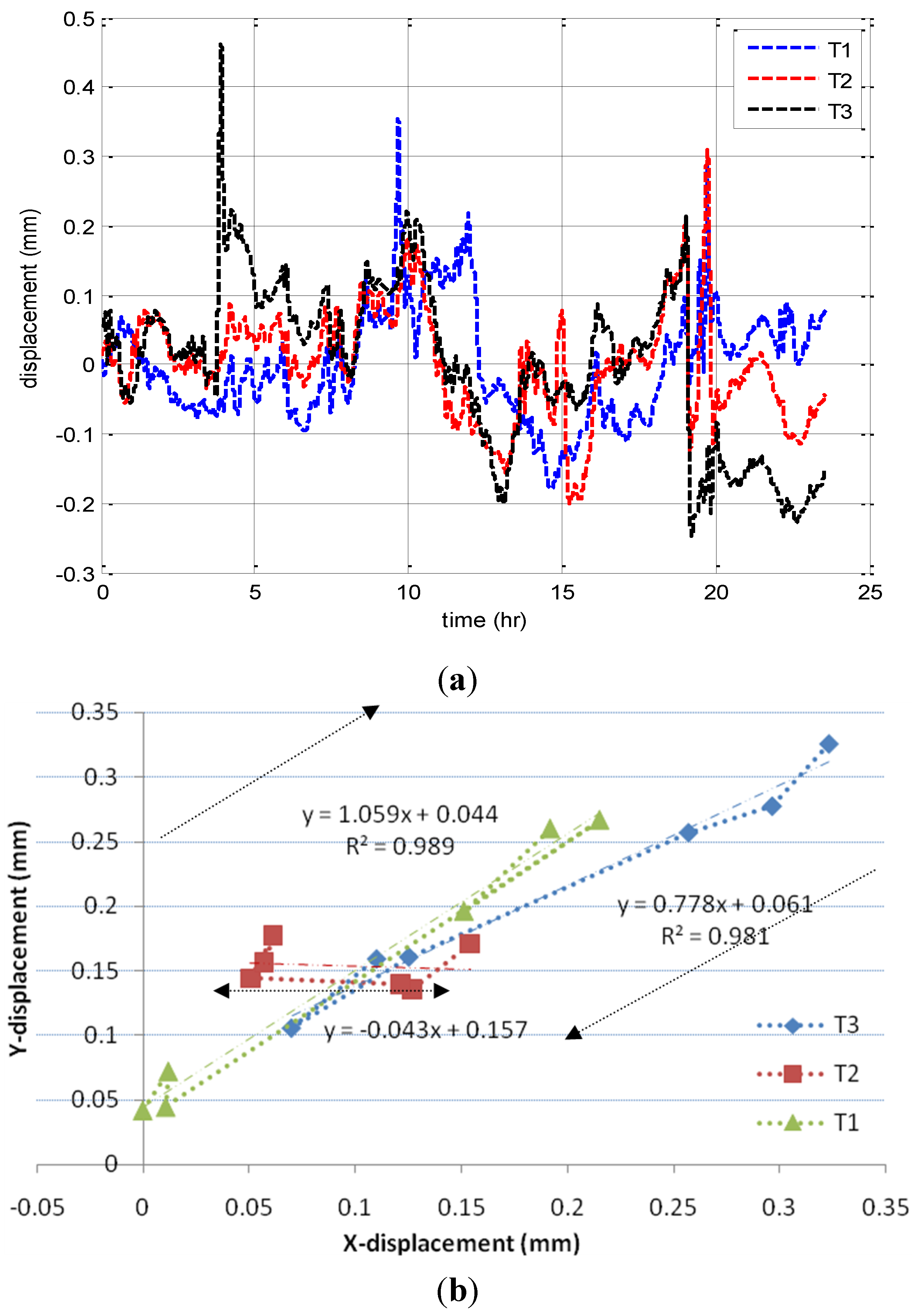
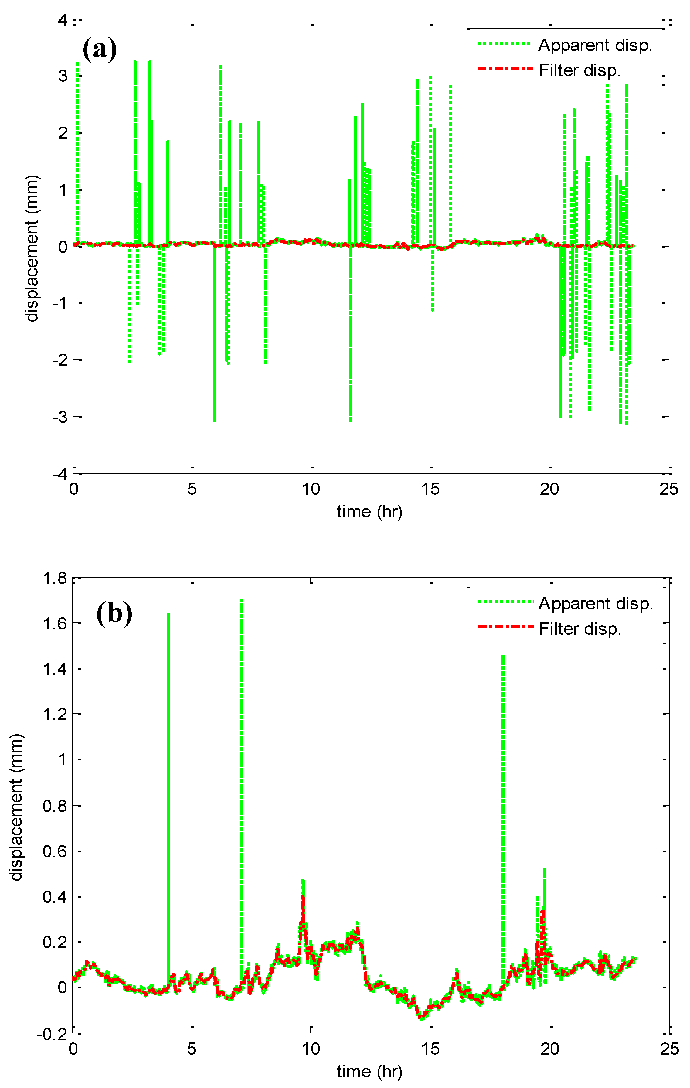
Figure 3. WT de-noising of GPS measurements of (a) Points 1 (Deck Point) and (b) T1 (Tower Point) in Y direction.

Figure 3. WT de-noising of GPS measurements of (a) Points 1 (Deck Point) and (b) T1 (Tower Point) in Y direction.

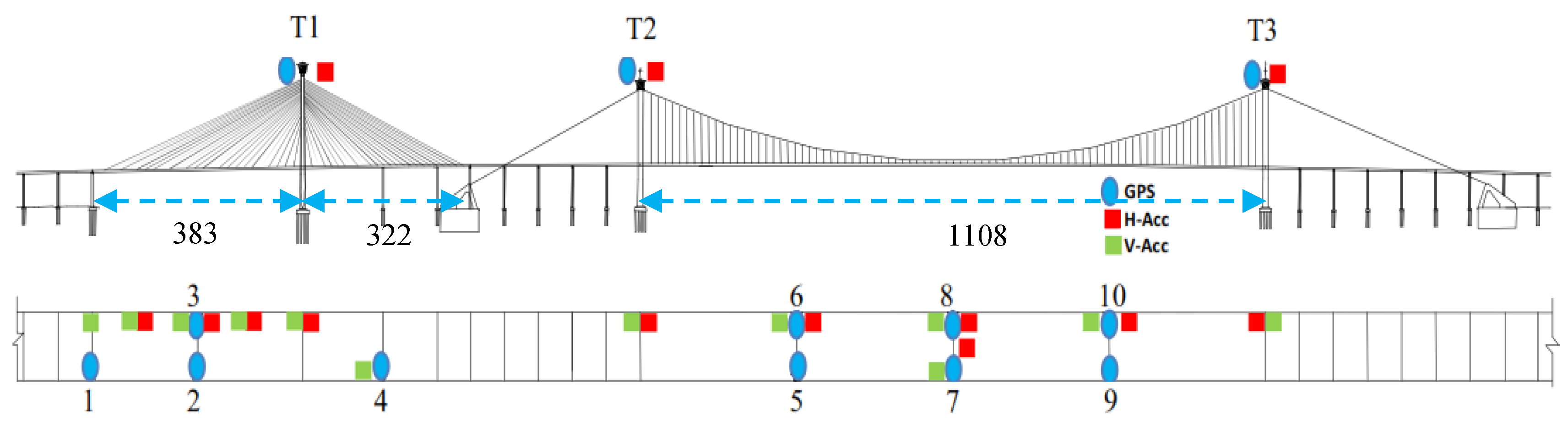
To verify this method, the wavelet de-noising of GPS measurements for the bridge deck and towers at points 1 and T1 (Figure 2) at 10 September 2009 is shown in Figure 3. Figure 3 illustrates that the wavelet method eliminates noise effects. In addition, it can extract the actual semi-static (slow change) movement component. It also can be used in calculating the dynamic (quick change) movement component based on the multi-filter method applied as described in Moschas and Stiros [10]. 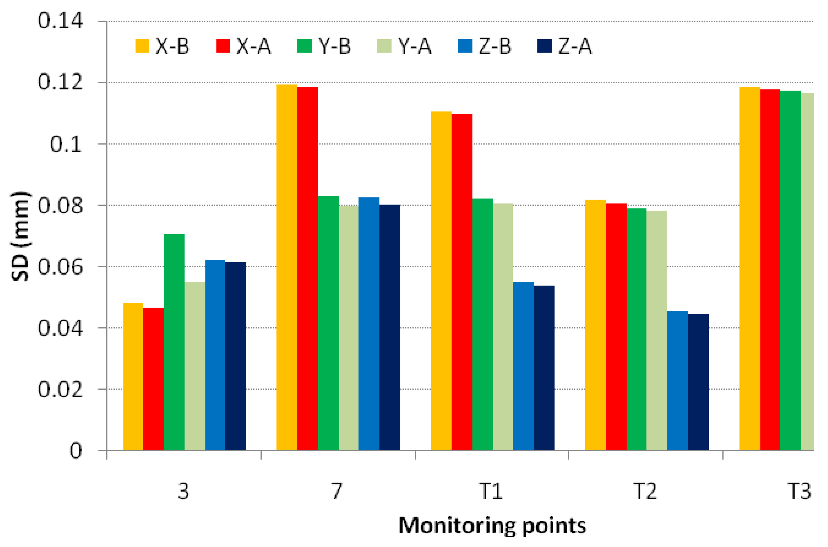Figure 4 depicts the standard deviation (SD) of measurements taken at the bridge deck and towers on 10 September 2009. The measurements were taken at deck points 3 and 7, and at tower points T1, T2 and T3, before and after applying the wavelet de-noising. It can be noticed that the wavelet method has removed the measurement noises and it also has increased the accuracy of the deck point’s measurements by 3.0% in the X and Z directions, and by 12.0% in the Y direction.

On the other hand, the accuracy of the towers points’ measurements has increased by 1.5% in the three orthogonal directions. These results imply that the GPS measurements at the deck points were noisier, due to GPS errors. Moreover, Figure 4 indicates that the tower measurements in the Z direction are negligible, while the displacements of the deck points are significant in all three directions.

Figure 4. GPS standard deviation of three direction measurements before (B) and after (A) WT de-noising.

Figure 4. GPS standard deviation of three direction measurements before (B) and after (A) WT de-noising.

4. ANFIS Movement Model Identification

The adaptive Neuro-fuzzy inference system (ANFIS) approach learns the rules and membership functions (MF) from training data [11,22]. ANFIS is an adaptive network of nodes and directional links through which the nodes are connected. It is called adaptive because some or all of the nodes have parameters which affect the node output. These networks identify and learn relationships between inputs and outputs. This is done by the fuzzification of the input through MF.

The parameters associated with input and output MF are trained using an algorithm, such as back-propagation and/or least squares [24]. Thus, unlike the multi-layer perceptron, where weights are tuned, in ANFIS fuzzy language rules or conditional (if-then) statements are determined in order to train the system. When “if” is [a set of antecedent conditions is satisfied], and “then” is [a set of consequences can be inferred], there are two basic components of all logical statements [11].For an ANFIS system to work appropriately in prediction mode, its initial structure and parameters (linear and nonlinear) must be tuned or adapted through a learning process, using a sufficient input-output pattern of data [16]. The basics for the fuzzy inference system (FIS) theory are defined in the reference Abdel-Hamid et al. [16].

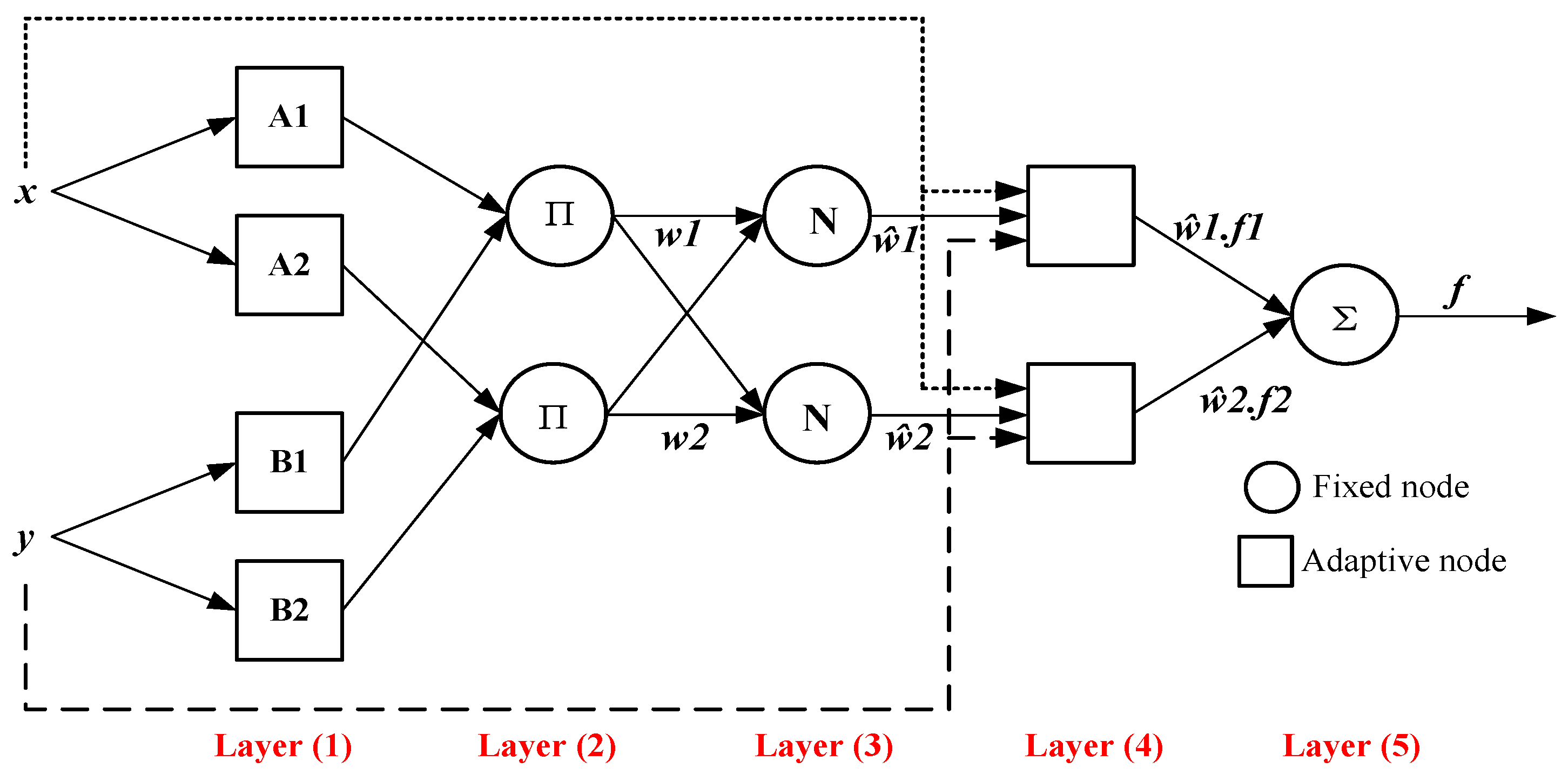
The general structure of ANFIS is presented in Figure 5, with two inputs (x and y) and one output (f). The adaptive layers are distributed between the antecedent and the consequent conditions. Moreover, it allows at the two conditions that the adjustments of their parameters and consequently the performance of the whole system [22,24].In this case, for the multiple-input, single-output (MISO) fuzzy system, the fuzzy rules for mapping linear functions of the inputs in the case of TS-FIS have the form:

R1: if (x) is A₁ and (y) is B₁, then

$$f_1=m_{1}x+n_{1}y+r_1$$

(9)

R2: if (x) is A₂ and (y) is B₂, then

$$f_2=m_{2}x+n_{2}y+r_2$$

(10)

where A and B are particular fuzzy subsets defined by a nonlinear coefficient, namely premise parameters, while m, n, and r are linear coefficients determining the output of each applied fuzzy rule and usually known as consequent parameters. The architecture of an ANFIS (see Figure 5) typically contains five layers, where the node functions (i) in each layer are of the same function family.

Layer 1: the input values are transferred to membership with respect to the different classifiers in the fuzzy input variable. However, the output node ($k_i^1$) is defined by:

$$k_i^1={\mu }_{Ai}(x)fori=1,2or{k}_i^1={\mu }_{Bi-2}(x)fori=3,4$$

(11)

Where ${\mu }_{Ai}$ and ${\mu }_{Bi-2}$ are the MF for the x and y inputs, respectively. The MF can be any appropriate function that is continuous and piece-wise differentiable, such as Gaussian, trapezoidal, triangle, or generalized bell shapes [11,12]. Investigating the statistical properties of different types of MFs shows that the root mean square error (RMSE) for the bell shapes are almost close values, while the RMSE for the generalized bell function is relatively small. Therefore, it is found that the suitable MF is the generalized bell function, which can be written for the first input, x, as follows (and similarly for the second input):

$${\mu }_{Ai}(x)=\frac{1}{1+\left|{(\frac{x-c_i}{a_i})}^{2b_i}\right|}$$

(12)

where (a_i, b_i, c_i) are the premise parameters that change the shapes of the MF with changed values [0, 1]; and they are the adjustable parameters in the premise condition.

Layer 2: the output memberships from layer 1 are used in this layer to determine the firing strength of each rule. They can be calculated as follows:

$$k_i^2=w_i={\mu }_{Ai}(x){\mu }_{Bi}(y)$$

(13)

Layer 3: the normalized firing strength is calculated in this layer, in order to calculate the weighted output estimate corresponding to each applied fuzzy rule:

$$k_i^3={\widehat{w}}_i=\frac{w_i}{{\displaystyle {\sum }_{j=1}^N{w}_j}}$$

(14)

where N denotes the number of the system input.

Layer 4: the weighted estimation output for this layer is a normalized firing strength by a first-order polynomial for the first-order TS method, and it can be expressed as:

$$k_i^4={\widehat{w}}_i{f}_i={\widehat{w}}_i(m_{i}x+n_{i}y+r_i)$$

(15)

where the consequent parameters (m_i,n_i,r_i) are adjustable and can be used to tune the output of that layer.

Layer 5: the sum of the weighted estimations results from the previous output layer is usually called defuzzification. It can be represented as follows:

$$k_i^5=f={\displaystyle {\sum }_{i=1}^N{\widehat{w}}_i{f}_i}$$

(16)

The premise (nonlinear) and consequent (linear) parameters of the FIS should be tuned to provide optimal representation of the factual mathematical relationship between the input and output spaces [16,24].

Figure 5. ANFIS architecture model.

Figure 5. ANFIS architecture model.

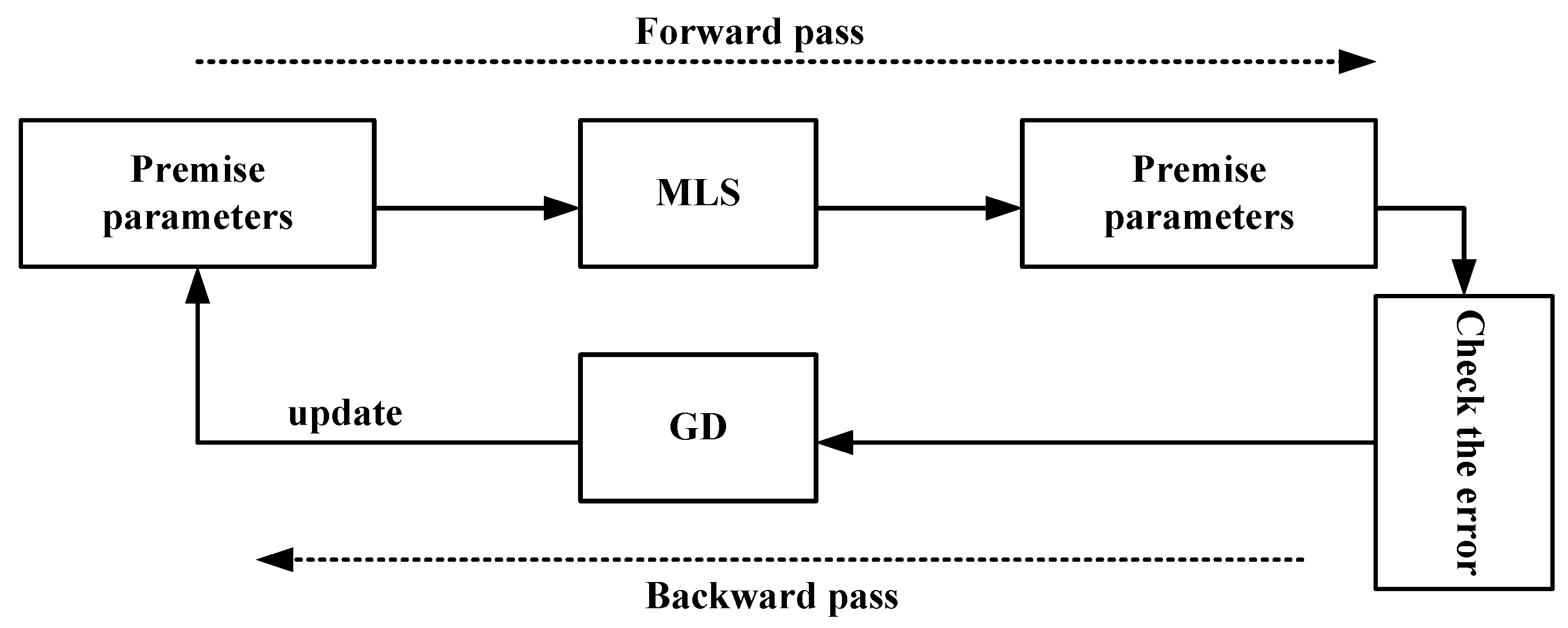
An approximate fuzzy model is initiated by the system and then improved through an iterative adaptive learning process. The training algorithm of ANFIS takes the initial fuzzy model and tunes it by means of a hybrid technique combining the gradient descent back-propagation and the mean least squares optimization algorithms [16,22,24]. This algorithm measures the model errors at each epoch, usually defined as the sum of the squared difference between actual and desired outputs, and reduces the errors. The gradient descent (GD) method is applied to adjust the nonlinear parameters, while the mean least square (MLS) method is used to optimize the linear parameters [16] as shown in Figure 6.

Figure 6. Hybrid ANFIS learning technique algorithm.

Figure 6. Hybrid ANFIS learning technique algorithm.

In this section, the prediction of the bridge deformations are studied and investigated. The GPS measurements taken on a single day (2September2009) for use as training data were selected as inputs for an ANFIS model. Correspondingly, in order to test and verify the model, the GPS measurements taken the next day (3September 2009) were also considered. All data were smoothed using the WT de-noising method. The extracted measurements at deck point 7, in the vertical Z axis, are used in this section. The coordinates of the measurements were transformed into a time series of apparent vertical displacements u around a relative zero representing the equilibrium level of the monitoring point. This similarity transformation is expressed as follows:

$$u(t)=z(t)-\frac{1}{n}{\displaystyle {\sum }_{t=1}^{n}z(t)}$$

(17)

where n represents the number of observations for one day’s monitoring data.

The present investigation model with product operator is chosen based on the executive FIS. The input data for the ANFIS model depends on the delay time to develop the performance model. Seo et al. [27] have applied the set of input variables to test the best delay time that can be used to improve the output model. Sudheer et al. [30] have used the statistical properties for the input data to select the standard input time delay of the model. In addition, multi linear regression (MLR) model isused to evaluate the degree of effect of each variable and to select the most effective input continues monitoring data [31,32]. Therefore, MLR model selection delay is applied in this study to select the effective time delay. Furthermore, three types of neuro-fuzzy networks are employed with different MFs. In the first network, the input data are considered as GPS monitoring data at current time (u(t)).In the second network, two depending values, which are the current and previous time (u(t) and u(t−1)), are considered. In the third network, three depending values (u(t), u(t−1), and u(t−2)) are considered. In each network, two, four, and six MFs are considered, with five epochs of training. The applied fuzzy rule base has two inputs for (x and y) as shown in Figure 5, and so on, for one and three inputs nodes.

Three types of standard statistical coefficients are used to perform the evaluation results. First, the correlation coefficients (R) defined as in Equation (18) and ranged between 0 and 1; where the higher the value of R, the better quality of the model. Second, the root mean square error (RMSE) defined as in Equation (19), where smaller value of RMSE means better quality of the model. Third, the mean absolute percentage error (MAPE) defined as in Equation (20) and used to verify the correctness of the models. The perfect value of MAPE is zero, representing the best fit of the model output to the observed values.

$$R=\frac{{\displaystyle {\sum }_{i=1}^n(u_i^o-{\overline{u}}_i^o)(u_i^p-{\overline{u}}_i^p)}}{\sqrt{{\displaystyle {\sum }_{i=1}^n{(u_i^o-{\overline{u}}_i^o)}^2{\displaystyle {\sum }_{i=1}^n{(u_i^p-{\overline{u}}_i^p)}^2}}}}$$

(18)

$$RMSE=\sqrt{\frac{1}{n}{{\displaystyle {\sum }_{i=1}^n(u_i^o-u_i^p)}}^2}$$

(19)

$$MAPE=\frac{100}{n}{\displaystyle {\sum }_{i=1}^n\left|\frac{u_i^o-u_i^p}{u_i^o}\right|}$$

(20)

Where $u_i^o$ and $u_i^p$ are the observed and predicted movement measurements at time i, respectively. Furthermore, the auto-correlation function (ACF) of the residuals $(e_t=u_i^o-u_i^p)$ is used to evaluate the model performance. The lag (m) auto-correlation (AC) is defined as in Equation (21).

$$\lambda (m)=\frac{1}{n}{\displaystyle {\sum }_{t=1}^n{e}_{t-m}{e}_t}$$

(21)

The AC λ(m) is zero when parameter model (k) is nonzero. A large AC when k is nonzero indicates that the residual is not zero-mean error and also implies that the model structure is irrelevant to the system, or that there might be a need to increase the model order. In real world applications, AC λ(m) cannot be zero when m is nonzero because of the limited length of observation points. If the value of AC falls within 95% of the confidence interval, the AC value is insignificant and this value is considered to be equal to zero.

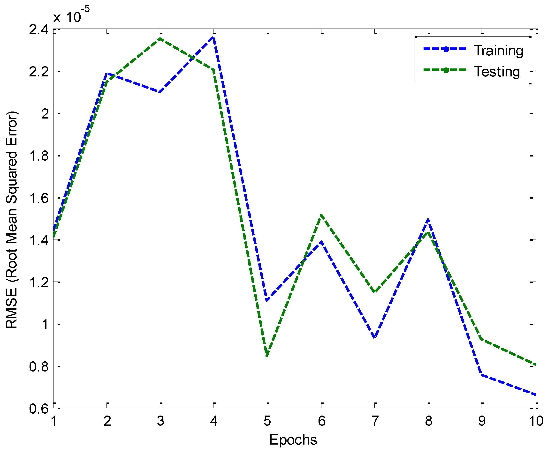
The model is implemented using the fuzzy logic toolbox in the MATLAB software package. The ability of the ANFIS model to achieve the performance goals depends on the predefined internal ANFIS parameters; however, the statistical properties of ANFIS model should be discussed first. The statistical study of bell shapes shows that the RMSE for the training data with generalized bell shape is 1.1 × 10⁻⁵ mm. Figure 7 illustrates the RMSE of training and test data with epoch number. From this figure, it can be seen that the RMSE has decreased after epoch number four. Therefore, in this study the epoch number that will be considered is five.

With the training dataset, we chose two generalized bell-shaped MFs for each of the inputs to build the ANFIS model. Table 2 illustrates the statistical errors of the training data for the prediction model, while Figure 8 represents the ANFIS model for the case of two inputs and MF. From Table 2, it is noticed that the MAPE values increase with increasing MF numbers, which refers to the immense decrease in the network nonlinearity. In addition, it is clear that the choice of two MFs for the two MISO cases is more suitable than the single-input, single-output (SISO) case. In addition, it shows that the SISO model has estimated high errors between the original and prediction data. Moreover, it can be seen that two inputs model is more suitable than three input models and consistent with this study. Table 2 results demonstrate that the commonly-used two MFs for time series prediction with u(t) and u(t−1) input structure is a suitable model, which can be used in this study. Therefore, the two multi-input single output model is suitable in this study.

Figure 7. Training and testing RMSE with epoch number.

Figure 7. Training and testing RMSE with epoch number.

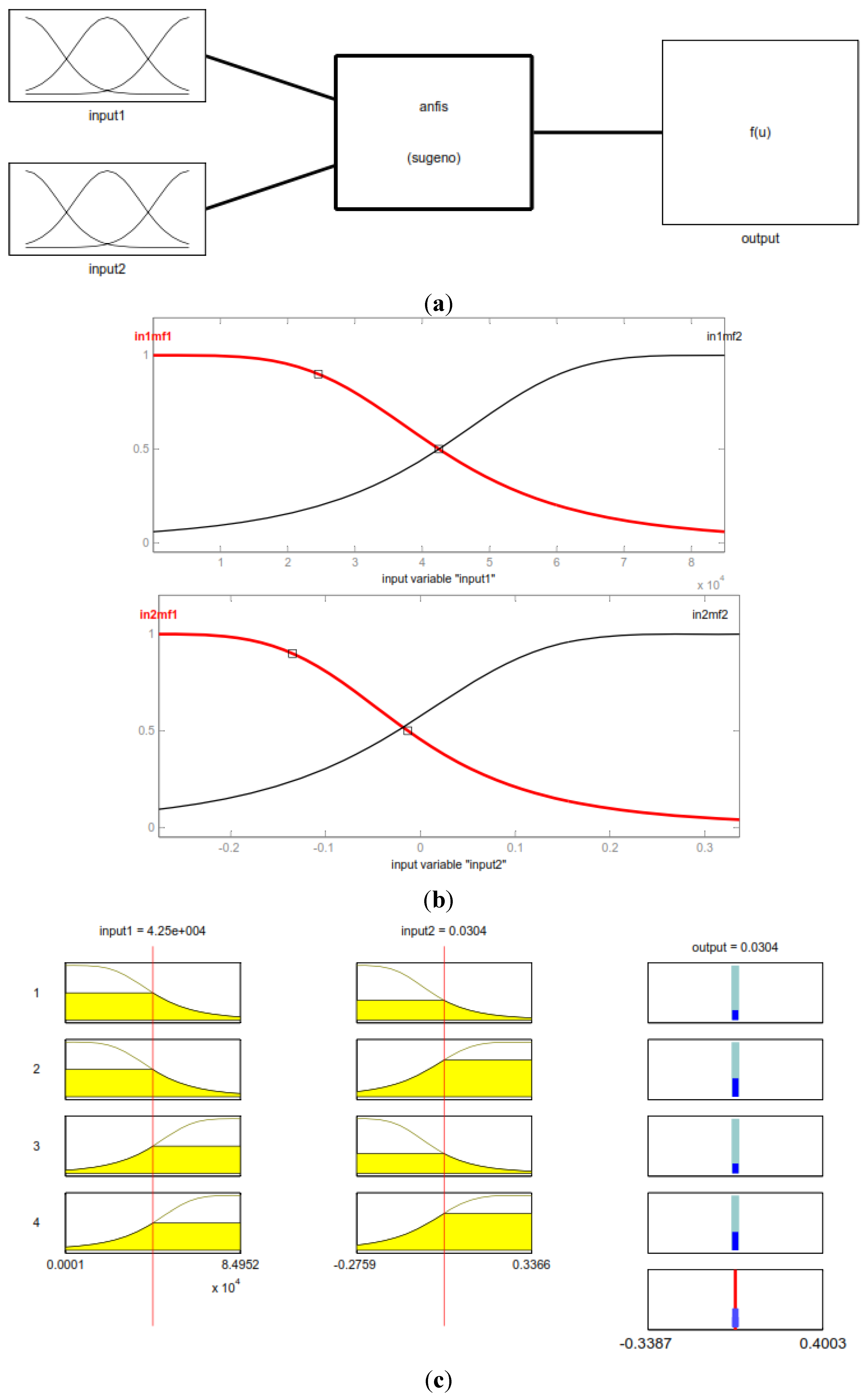
Figure 8 presents the model used. This model leads to four “if-then” rules containing 24 parameters to be learned. Figure 8a shows the ANFIS model to be built for the GPS real-time monitoring measurements assessment in this study. The premise parameters of the input layer are calculated and the adjusted MFs for the two inputs are shown in Figure 8b. It can be seen that significant modifications have been made to the shape of the initial MF through the learning process. The Takagi-Sugeno (TS) model is applied and the consequent parameters are evaluated.

Table 2. Error analysis of monitoring GPS training data.

Input Manners	No. of MF	MAPE (%)	RMSE (mm)	R
u(t)	2	790.123	0.98× 10−1	0.169
	4	1807.471	1.61× 10−1	0.015
	6	1135.017	1.18× 10−1	0.037
u(t) and u(t−1)	2	1.15	2.57 × 10−4	0.999
	4	8.945	0.62× 10−1	0.653
	6	58.11	3.45× 10−1	0.472
u(t), u(t−1), and u(t−2)	2	2.363	4.69 × 10−4	0.999
	4	7.036	0.33× 10−1	0.904
	6	55.103	5.14× 10−2	0.770

Table 2. Error analysis of monitoring GPS training data.

Input Manners	No. of MF	MAPE (%)	RMSE (mm)	R
u(t)	2	790.123	0.98× 10−1	0.169
	4	1807.471	1.61× 10−1	0.015
	6	1135.017	1.18× 10−1	0.037
u(t) and u(t−1)	2	1.15	2.57 × 10−4	0.999
	4	8.945	0.62× 10−1	0.653
	6	58.11	3.45× 10−1	0.472
u(t), u(t−1), and u(t−2)	2	2.363	4.69 × 10−4	0.999
	4	7.036	0.33× 10−1	0.904
	6	55.103	5.14× 10−2	0.770

The application of the ANFIS system is presented in Figure 8c, which includes the five basic steps of the calculation. The system starts with the fuzzification of the inputs, where each input is processed in parallel through the membership functions. Second, the rules are applied using the fuzzy operator (AND) which results in the weighted firing strength to the third part of the implication and transfers data from the premise to the consequent. The fourth step is the aggregation of the consequents across the rules, and the final step is the defuzzification of the results to produce the final output.

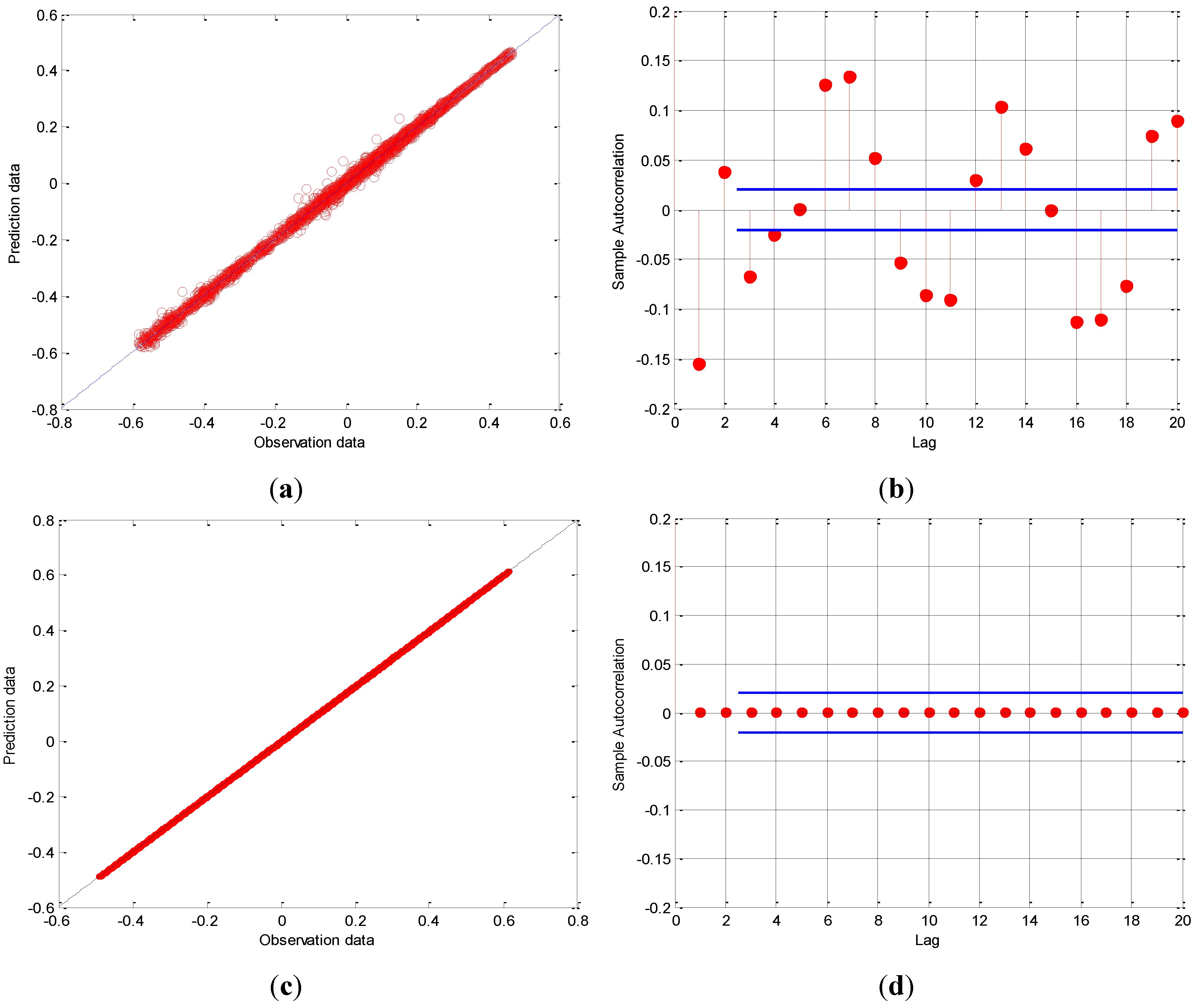
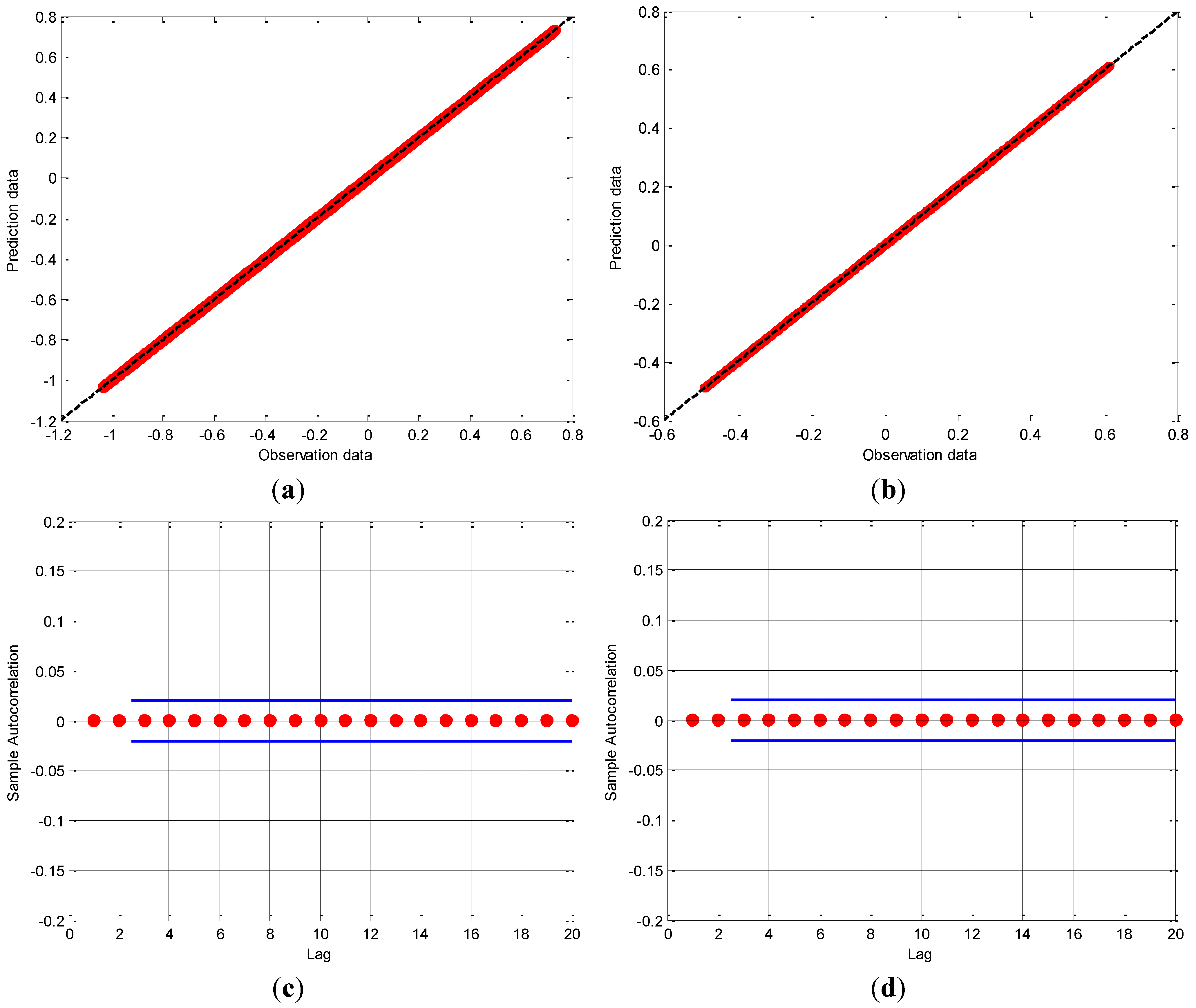
Herein, to evaluate the applicability of the wavelet method, the performance of ANFIS model using de-noising input data is compared with that of ANFIS model using original input data (without de-noising), as shown in Figure 9. Figure 9a,c shows the prediction values using the ANFIS model and the monitoring measurement of testing data with exact fit for the original and de-noising signals, while Figure 9b,d depicts the sample auto-correlation function (ACF) for the estimated model errors. From Figure 9, it can be seen that the prediction values are very close to the test data values in the two cases, i.e., before and after applying the wavelet method. In addition, the correlation between the exact fit and data is very high. The residual of the model prediction is shown to be within and out the 95% ACF confidence interval in the case of de-noising and original signals, respectively. In addition, it can be seen that MAPE is 0.12 and INF %, RMSE is 1.33×10⁻³and 4.46×10⁻² mm, and R is 0.99 and 0.95 for the prediction testing data after and before de-noising, respectively. The comparison between the ANFIS model results in the two cases for the signals refers that the wavelet method is significant to remove the noise effects and to improve the ANFIS prediction data. Furthermore, these results indicate that no information losses are detected for the prediction model with applying the wavelet method, and also confirm the high safety of the performance of the bridge. Therefore, the model is recommended to be used in the efficient prediction and assessment of the deformations of bridges after removing the noise effect.

Figure 8. The (a) design model, (b) MF adjustment and (c) model application of two MF and two inputs time series ANFIS prediction model.

Figure 8. The (a) design model, (b) MF adjustment and (c) model application of two MF and two inputs time series ANFIS prediction model.

Figure 9. The ANFIS prediction movement for the GPS measurements (a) before and (c) after wavelet filter applied and ACF for the test monitoring data (b) before and (d) after filter applied.

Figure 9. The ANFIS prediction movement for the GPS measurements (a) before and (c) after wavelet filter applied and ACF for the test monitoring data (b) before and (d) after filter applied.

5. Bridge Performance Analysis

5.1. Monitoring Data Analysis

In this section, the movements of the bridge deck and towers are analyzed, based on the GPS’s and the accelerometers’ measurements. Two monitoring points at the mid-span of the deck (points 3 and7) are selected.

5.1.1. Deck Monitoring Points

Figure 10a,b demonstrate the similarity transformation displacement (see Equation (16)) of the smoothed measurements of deck monitoring points 3 and 7 on 10 September 2009. The statistical displacement range for the same monitoring points on 5, 10, 15, 20, and 25 September 2009 is shown in Figure 10c. Figure 10 illustrates the high efficiency of the WT de-noising in smoothing and eliminating the noises from the GPS measurements at the deck monitoring points. It can be concluded that the maximum displacement range in the three directions took place at point 7. In addition, high correlation (0.85) between displacement ranges is shown for point 3. This indicates more stability at point 3 due to the bridge span length effect.

It can be seen that the maximum displacement range for point 7 took place in the Y and Z directions on 15 September 2009, while it occurred in the X and Y directions on 25 September 2009. Therefore, displacements of point 7 occurred in all three measurements directions, while the main difference between the measurements relates to the varying traffic load with time. However, point 7 suffered more significant movements compared to the other bridge monitoring points. In addition, the displacement range value indicates the safety of the bridge in the static and semi-static movement behaviors.

The fundamental frequency (first mode frequency) of the acceleration measurements of point 7 shows that the fundamental frequency differences are negligible for the various monitoring days. The fundamental frequencies of point 7 for all the monitoring days are 0.585 Hz, 0.585 Hz, and 0.1953 Hz for the X, Y, and Z directions, respectively.

5.1.2. Towers Monitoring Points

Figure 11 illustrates the WT de-nosing of the GPS measurements of the three monitoring points in the bridge towers on 10 September 2009, as well as the mean displacements on 2, 5, 10, 15, 20, and 25 September 2009, for the three points. From Figure 11, it can be seen that the correlation coefficients between T1 and T2, T1 and T3, and T2 and T3, are 0.30, −0.04, and 0.63, respectively. This indicates a high correlation between the measurements taken at the two monitoring points on the towers of the suspension bridge. The results imply a poor correlation between the measurements taken at the tower of the cable-stayed bridge portion and the adjacent tower of the suspension bridge portion. No correlation is shown between the measurements taken at the tower of the cable-stayed bridge portion and the far tower of the suspension bridge portion. The displacement range (mm) for measurements taken at T1, T2, and T3 are (0.215, 0.225), (0.104, 0.042), and (0.253, 0.220), for the (X, Y) directions, respectively.

Figure 11a explains that the maximum displacements of the three monitoring points on the towers occurred three times, while the maximum range displacement for point T3 exceeds that of both T2 and T1. This result suggests that the long spans of the suspension and the cable-stayed bridge portions affect the movement of the towers differently. Figure 11b describes the three towers’ displacements in both the X and Y directions. It can be seen that the displacements of the external towers (T1 and T3) are within the displacement range of the inner tower T2, while the T2 movement can be assumed in the X-direction only. In addition, the linear fitting of displacements shows that the movements of points T1 and T3 are approximately linear. It can be seen that the high closed mean values of displacements occurred during the monitoring days of 15, 20, and 25 September 2009. It means that the low displacements and, therefore, the safety of the towers in two directions occurred during the monitoring time in the static and semi-static movement’s components.

The fundamental frequency results of the accelerometer measurements of the three towers’ monitoring points show that the fundamental frequency of these points are almost identical in the X and Y directions during the different monitoring days, and are equal to 0.5859 Hz.

Figure 10. Displacement time series of bridge deck on 10 Sept. for (a) point 3; (b) point 7 and (c) Displacement range of GPS measurements.

Figure 10. Displacement time series of bridge deck on 10 Sept. for (a) point 3; (b) point 7 and (c) Displacement range of GPS measurements.

Figure 11. (a) The time series of Displacement in Y-direction and (b) scattered of GPS measurements for the three towers of bridge(the arrows refers to the movement direction).

Figure 11. (a) The time series of Displacement in Y-direction and (b) scattered of GPS measurements for the three towers of bridge(the arrows refers to the movement direction).

5.2. ANFIS Prediction Performance Model Analysis

Figure 12 represents the design performance model of the bridge based on the ANFIS system with WT de-noising GPS measurements. In this section, for the GPS-bridge movement performance, the GPS measurements taken on 2 September 2009, are used as the reference for monitoring the movement data, while the measurements taken on 15 and 25 September 2009 are used as the check data to analyze the performance of the bridge during those days. Based on the analysis of measurements in the previous section, it was noticed that the most critical point was point 7, which is located on the bridge deck. This monitoring point has a high range of movement.

Figure 12. GPS prediction model performance analysis.

Figure 12. GPS prediction model performance analysis.

Figure 13. TheANFISPrediction movement performance on (a) 15 Sept.; (b) 25 Sept. and ACF for the check time on (c) 15 Sept.; (d) 25 Sept. of ANFIS model design.

Figure 13. TheANFISPrediction movement performance on (a) 15 Sept.; (b) 25 Sept. and ACF for the check time on (c) 15 Sept.; (d) 25 Sept. of ANFIS model design.

In this section, the measurements taken in the Z direction are selected for the checking of the performance of the bridge. The movement prediction and ACF check prediction error are shown in Figure 13. Table 3 shows the predicted statistical performance for the prediction errors. From Figure 13 and Table 3, it can be seen that the prediction model results are highly correlated with the monitoring measurements of the bridge. In addition, the auto-correlation significance of prediction error is shown to be within the 95% confidence interval for the two monitoring check days. This means that there were no information losses for the movement’s prediction data. Furthermore, the statistical analysis results in Table 3 indicate that the check errors of the two monitoring days are insignificant. It can be concluded that the performance of the bridge deck during one month of continuous monitoring is very safe in the time and frequency analysis.

Table 3. Statistical performance monitoring check dates.

Monitoring Date	MAPE (%)	RMSE (mm)	R
15 September 2009	0.113	1.85 × 10 −3	0.999
25 September 2009	0.121	1.33 × 10 −3	0.999

Table 3. Statistical performance monitoring check dates.

Monitoring Date	MAPE (%)	RMSE (mm)	R
15 September 2009	0.113	1.85 × 10 −3	0.999
25 September 2009	0.121	1.33 × 10 −3	0.999

The design performance of the ANFIS model supports the same result. In addition, the prediction model is found to be suitable and can be applied, with future monitoring data, to check the performance of the bridge directly under different loads. It is found that the ANFIS method is a good choice and a powerful tool for modeling the performance of bridges. This result is consistent with the results obtained by Pantazis and Alevizakou [20].

6. Conclusions

Through a careful inspection of the results that are presented in this study, certain remarks can be made and conclusions extracted.

The application of the wavelet transform (WT) de-noising method demonstrates a powerful filter tool for de-nosing and, hence, smoothingthe GPS measurements, without any loss of information in the static and semi-static components of movements. In other words, the results of the measurements taken at the monitoring points located on the towers and the deck of the Huangpu Bridge demonstrated the ability of the WT de-noising method to reconstruct GPS measurements, while keeping the accuracy of the measurements consistent.

The adaptive neuro-fuzzy inference system for the output RTK-GPS long-term monitoring system was applied for predicting the GPS movements of the bridge deck monitoring points. Three types of neuro-fuzzy networks were considered regarding the input variable patterns, while each network was executed with two, four, and six membership functions. For attaining this purpose, one day’s GPS measurements of the monitoring point on the deck were used.

The proposed results of the adaptive neuro-fuzzy inference system method provided a reliable movement estimation, which can be used to assess the performance of the monitoring point. In addition, it was found that the two-membership function is suitable and fast to apply with two input variables. The residual of the testing prediction data is shown to be within the 95% confidence interval forthe auto-correlation function. The proposed method can be concluded as the method, which learns the “if-then” rules between past input bridge displacements and memorizes them for the generation and prediction of future displacements. In addition, it was found that the ANFIS model is a good and sufficient toolfor use in predicting structural deformation.

Analysis of the structural health monitoring data shows that the Huangpu Bridge is safe, to judge from the different movement components, which are the static and the semi-static components based on RTK-GPS measurement, plus the dynamic component based on accelerometer measurements. The static and semi-static displacements components are relatively small, and the components of the dynamic frequency are approximately constant at the different monitoring times.

Finally, the performance analysis of the design prediction model illustrates that the auto-correlation function residuals for the check time data are within the 95% confidence interval for the auto-correlation function, and that the statistical errors for the check times are small. These results indicate that the Huangpu Bridgeis safe during the study’s monitoring times.