Improving Post-Earthquake Insurance Claim Management: A Novel Approach to Prioritize Geospatial Data Collection

Abstract

With a population exceeding 14 million and a GDP of more than 300 billion USD, Istanbul dominates the Turkish economy. Unfortunately, this concentration of social and economic assets is permanently threatened by potentially devastating earthquakes, given the city’s close proximity to several well-known fault systems. As a measure to mitigate the consequences of such events, and to increase the resilience of the exposed communities, the Turkish Catastrophe Insurance Pool (TCIP) has been set up to provide affordable and reliable earthquake insurance to households all over the country. In the aftermath of a damaging event, especially in Istanbul, the operational capacity of TCIP will be seriously challenged by the high number of claims whose settlement would have to be swift and fair in order to kick-start the recovery process. In this paper we explore an integrated approach based on mobile mapping and ad hoc prioritization techniques to streamline the data collection and analysis process, with application to both the pre-event and post-event phases. Preliminary results obtained in Besiktas, a populous district of Istanbul, are presented and discussed.

1. Introduction

With a population exceeding 14 million and a GDP of more than 300 billion USD, Istanbul is the major driver of the Turkish economy. Unfortunately, this concentration of social and economic assets is constantly threatened by potentially devastating earthquakes, as the city is close to several well-known fault systems. Turkey is, in fact, located in one of the most active earthquake regions in the world. There is clear evidence for several significant earthquakes (magnitude greater than 7) happening in the last 2000 years in the eastern Marmara region [1], and in the recent past we have already witnessed large-scale disasters. In particular, on 17 August and 12 November 1999, two earthquakes occurred in the western extension of the North Anatolian fault, causing more than 15,000 casualties in the towns of Izmit and Gölcük, with more than 300,000 housing units destroyed or damaged and more than 600,000 people displaced [2]. The impact of this earthquake was also significant in economic terms, with a cost of between 5 and 14 billion USD [3]. There is general agreement among the researchers that a large seismic event could strike this area in the near future [1,4,5,6]. A magnitude 7.5 strike-slip earthquake occurring on the Marmara fault, considered a worst-case scenario compatible with the local seismic hazard [4,6,7], could cause up to 30,000 to 40,000 fatalities and possibly result in more than 30% of the overall building stock being moderately or extensively damaged [7,8]. Among the prevention and mitigation measures adopted by the Turkish government in the aftermath of the 1999 disasters is the establishment of the Turkish Catastrophe Insurance Pool (TCIP), a public sector insurance entity whose mission is to provide catastrophe risk insurance to homeowners at national level [9]. The main objectives of TCIP are:

• the provision of affordable earthquake insurance coverage for all urban dwellings,
• the limitation of the government’s financial exposure to natural disasters,
• the improvement of risk reduction and mitigation practices in residential construction.

Since its foundation in the year 2000, TCIP has achieved a 39.5% penetration rate in Turkey, with more than 6.9 million policies, and a 51.1% penetration rate in Istanbul with 1.9 million active policies (Source: TCIP). With a short-term forecast of reaching 10 million policies by 2020, equivalent to a national market share of about 55%, TCIP has already produced a massive increase in the risk awareness of the population, and has inspired several other earthquake-prone countries to launch similar programs [9].

Despite these encouraging figures, the occurrence of a powerful earthquake in a high-density metropolitan area would seriously challenge the operational capabilities of TCIP to efficiently settle the related claims. Since 2010, TCIP has successfully managed more than 10,000 claims, with a single event (the 2011 Van earthquake) totaling alone 8700 claims. However, a M7+ event in the Istanbul area, as mentioned above, could generate an astounding 300,000 claims in a few weeks [8,10], an overwhelming number that would require years to be settled.

When analyzing the internal claim management process, a potential bottleneck was found in the inspection procedure, which requires an experienced operator to physically visit the building hosting the related policy to assess the actual level of damage. While this procedure is suitable to a routine claim management, it would be unfeasible for a massive event, requiring thousands of operators working concurrently in the field. The necessity of a more efficient methodology for policy-related data collection in order to streamline the claim management process is evident from the above considerations, and requires innovative approaches in order for this issue to be tackled properly.

This paper describes a novel approach for the prompt collection of geo-localized visual information of the damage state of the buildings hosting insurance policies, which would considerably streamline the claim management process. The proposed approach is based on the use of a lightweight mobile mapping system to collect geo-referenced omnidirectional images of the affected urban environment, which would then be analyzed off-line. Splitting the in situ data collection from the actual analysis of the collected images, would have a number of advantages:

• a partial shift in the burden of inspection to an offline procedure, which could be conveniently scaled up or down by involving a pool of skilled operators operating from remote;
• less risk for the in situ operators to be affected by aftershocks or structural collapses, as it would generally involve less interference with recovery operations;
• a simple technical solution for visual data collection would not require expert operators and could be quickly deployed and operated on the ground;
• the same approach could be used pre-event to collect reference images, thereby capturing further information useful for the post-event claim settlement process.

Within this scheme, the critical role of geo-information and geographical information systems has to be acknowledged. In this framework, a methodology for the prioritization of data collection is introduced, based on the combination of two or more geo-information layers encoding different indicators of sampling importance (referred to as focus maps [11] and described below).

The survey and collection of geo-spatial data, i.e., geo-localized information, can be considered equivalent to the statistical characterization of a population whose elements are of interest for the purpose of the survey. Often the dimension of the population, or the burden associated with the data collection itself, are incompatible with a full enumeration and characterization of the elements. If we consider, for instance, the task of inspecting the residential areas in Istanbul in order to map the damage distribution (or to characterize their vulnerability in a pre-event phase), it is clear that a full-scale survey of the 800,000+ buildings would require significant resources. In these cases, a statistical characterization based on the sampling of the underlying population should be applied. Moreover, if we consider the task of inspecting buildings for the assessment of the damage state in a post-event application, the limited time frame (important to guarantee a swift settling of claims) represents an additional constraint. The inspection of a much smaller number of elements of the population, followed by an extrapolation (inference) of the characteristics of interest would make the task feasible within a reasonable time frame [12]. The practical necessity of characterizing only a small number of elements, and perhaps over subsequent collection stages, calls upon the development of optimization approaches that would answer the following question: “What elements should be accessed first in order to achieve an optimal trade-off between the uncertainty of the overall estimates and the time and cost of the survey itself?” We refer to such an approach as optimization and prioritization of geo-spatial data collection.

In the considered context, prioritization refers to selective sampling operations which realize a statistical characterization of a population of interest (in our case the population is defined by the buildings that hold one or more earthquake insurance policies) and optimize the use of available resources in order to comply as closely as possible to existing constraints. From the geo-statistic point of view, this is closely related to applying an adaptive spatial sampling [13,14] with unequal probability [15]. In the literature, a few references can be found on the use of a priori information to improve sampling, mostly connected to the characterization of environmental resources. For instance, [16,17,18] exploit remote sensing and other ancillary geo-information to optimize the sampling design of cropland areas, the monitoring of land cover or the delineation of watersheds. In the field of Disaster Risk Reduction and Risk Management, while the value of geo-information is being increasingly recognized [19,20] and the use of Geographical Information Systems (GIS) is widespread [21], the application of sound statistical frameworks to optimize the collection of relevant in situ information is limited, and the concept of prioritization mostly refers to the selection of hotspots for natural disasters (see, for instance, [22]).

The combination of prioritization approaches and mobile mapping technology proposed in this paper has been tested in a representative site in Istanbul (Turkey). The considered study area is introduced in Section 2. In Section 3 the proposed approach for rapid data collection and the prioritization strategy are described. The custom-made mobile mapping system employed in the field activities is briefly described in Section 4. The results of the preliminary activities are presented in Section 5 and expanded upon in Section 6, with conclusions outlined in Section 7.

2. Study Area and Data

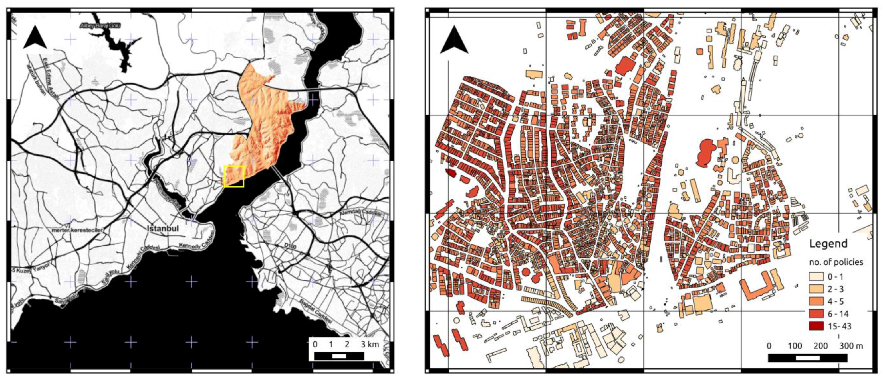
The Besiktas district of Istanbul, Turkey (Figure 1, left), located on the European shore of the Bosporus, has been selected as a study area. It is bordered on the north by the Sariyer and Şişli districts, to the west by Kağıthane and Şişli, to the south by Beyoğlu, and on the east by the Bosporus. The Besiktas district covers an area of around 20 km² with approximately 186,000 inhabitants in 2012, leading to an average population density of 9300 people/km². Besiktas exhibits a diverse composition of different building types that can be considered representative of the larger Istanbul area. A detailed description of buildings’ typology and physical vulnerability in Istanbul can be found in [4].

The total number of policies present in the Besiktas district (in 2013) amounts to 29,832, with an average of 1492 policies per km². Forty-four percent of the buildings (8421) reported in the district host at least one policy, with an average of 1.56 policies per building and a maximum of 155 policies for a single building. It can be noted that the distribution of policies is rather sparse, since 95% (8054) have fewer than 10 policies, and 67% (6132) of the buildings have fewer than 5.

Figure 1. Overview of the study area Besiktas, Istanbul, Turkey (left); zooming in (yellow rectangle in the left map) on the distribution of buildings and related earthquake insurance policies in the Besiktas district (right).

Figure 1. Overview of the study area Besiktas, Istanbul, Turkey (left); zooming in (yellow rectangle in the left map) on the distribution of buildings and related earthquake insurance policies in the Besiktas district (right).

Figure 2. Distribution of policies with respect to buildings’ usage (left), and relative distribution of apartments and offices in the test areas (right).

Figure 2. Distribution of policies with respect to buildings’ usage (left), and relative distribution of apartments and offices in the test areas (right).

The input datasets that were used in this study include a complete building and road inventory, a probabilistic seismic hazard map, and a Digital Elevation Model (DEM), provided by TCIP. The building inventory with information on existing policies contains the footprints of 19,158 buildings, each with information on the number of policies, the type of construction, number of stories, type of usage (residential, mixed residential and non-residential), number of apartments and offices, and number of parking lots (see Figure 1, right, and Figure 2). The vectorial road inventory covers 380 km, with each road segment including attribute information about the road type, width, and number of lanes. The road network has been topologically corrected and converted into a routable geometric network with additional attributes defining the directivity and cost factors for traveling along street segments. The considered probabilistic seismic hazard map is estimated both in terms of Peak Ground Acceleration (PGA) and Peak Ground Velocity (PGV) with an exceedance probability of 10% in 50 years and defined over a regular grid. Moreover, a raster layer estimating the susceptibility level of road blockages in case of an earthquake has been provided for the considered area. Both raster layers are defined on an equally spaced grid with a cell size of 0.2 km² (approximately 0.04° longitudinal, 0.05° latitudinal resolution). A DEM is available for the study area with a horizontal resolution of 1 m. The DEM has been integrated with the 3D geometry information of the building inventory (footprint and estimated height) to derive a digital surface model (DSM).

3. Prioritizing Geo-Spatial Data Collection

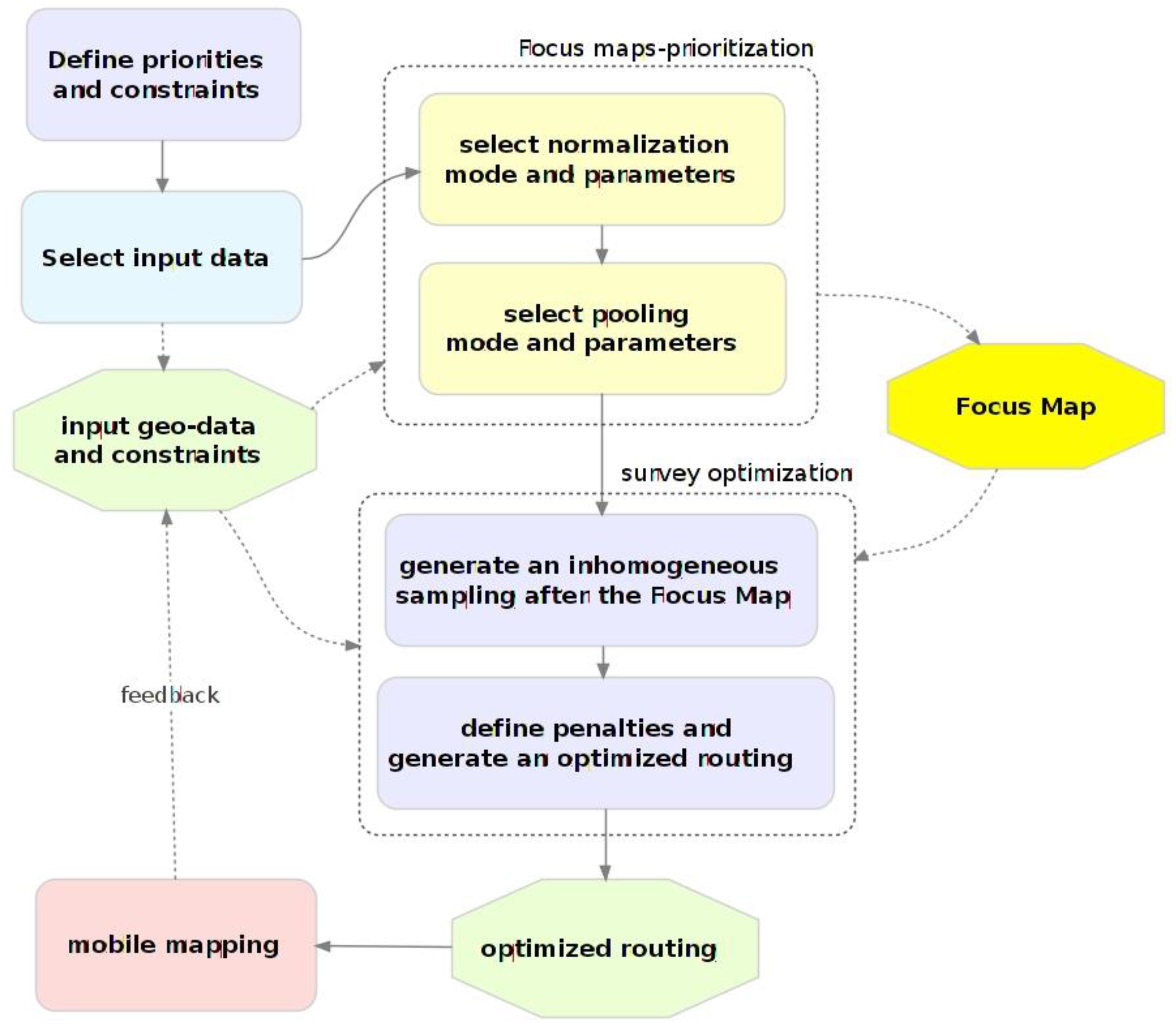
The proposed approach is based on the integration of prioritization and optimization stages in an iterative scheme. The general work-flow of the implementation stages, sketched out in Figure 3, entails a first phase where priorities and constraints are collected in the form of geo-spatial layers. The prioritization of the data collection is realized by using the collected information to generate a raster map to give the above-mentioned focus maps [11]. Focus maps combine different geo-information layers representing individual criteria into a single raster representing the inclusion probability of each point, that is, the probability of the point being selected for surveying conditional on the sampling probability of each of the other layers (probability pooling). This in turn drives the subsequent data collection phase. In order to implement an efficient survey based on the use of a mobile mapping system, a set of sampling points is generated according to the computed focus map, and suitably routed on the existing road network. This allows one to realize the further optimization of the overall data collection by encoding additional survey constraints in the routing algorithm.

The mobile mapping system is then deployed and driven according to the planned route. The georeferenced, omnidirectional images collected during the survey can be suitably analyzed by one or more operators, and the extracted information stored in a geo-database. Moreover, the outcomes of the survey can be used to repeat the prioritization and optimization process by accounting for both the original constraints and for the information collected in the field, therefore realizing an iterative, incremental data collection process.

3.1. Prioritized Sampling

The first prioritization stage is based on the above described concept of focus maps [11]. In order to compute the focus map, each of the input layers is mapped (normalized) into a sampling probability. This mapping can be either linear or non-linear (see [11] for examples) and is selected by associating sampling probabilities to locations according to the value assumed by the layer itself. For instance we can consider as input layers the distribution of insurance policies. The mapped layer will exhibit higher sampling probabilities where the spatial density of policies is higher. The mapped layers, now defining different sampling probabilities, can be combined by a pooling procedure. The pooling can be multiplicative, additive, or mixed, depending on the way the joint sampling probability should be implemented; a multiplicative pooling will associate small sampling probabilities to locations where at least one of the input layers has a low probability. Conversely, additive pooling will associate higher sampling probability where at least one of the input layers has high probability. By changing the weights (keeping the sum of the weights to 1), the relative importance of the datasets also changes. With log-linear pooling, the weights can be further increased in order to make the resulting survey more selective. As the absolute values of the weights increase (keeping constant the relative ratio), only the highest values (thus indicating a higher priority) are retained (see Figure 4).

Figure 3. Diagram showing the prioritization work-flow with iterative multi-stage sampling.

Figure 3. Diagram showing the prioritization work-flow with iterative multi-stage sampling.

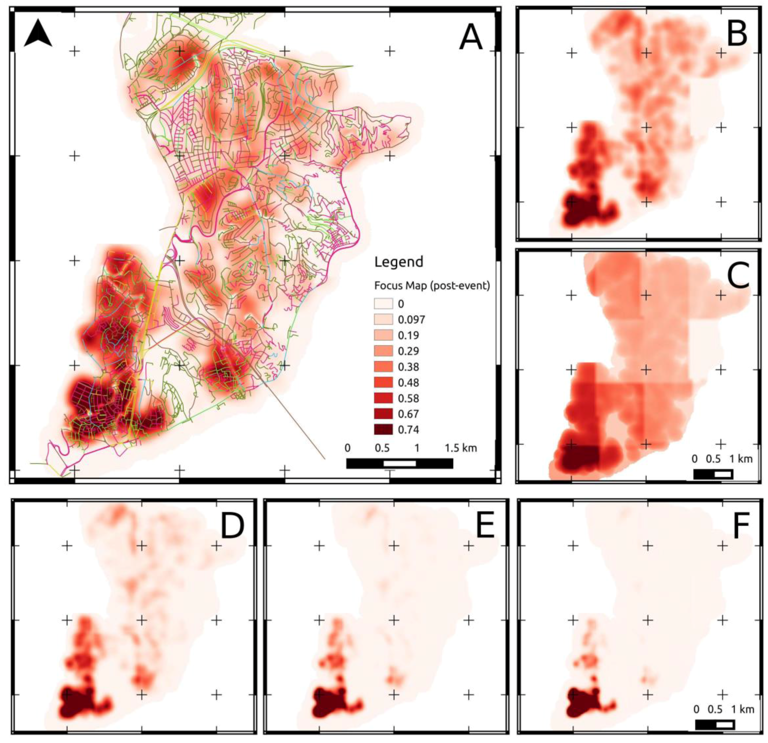
Different focus maps, based on different input layers, can be implemented to drive the optimization and prioritization of the data collection, according to the specific operational stage. In order to analyze the building stock in a pre-event stage, the expected distribution of seismic hazard could be combined with the density of insurance policies and the distribution of buildings. An example of a pre-event focus map is provided in Figure 4. For post-event damage assessment, a preliminary distribution of physical damage obtained by remote sensing or direct inspection could be combined with the expected distribution of road blockages.

Once the focus map is computed, it can be used to generate a set of sampling points in the area to be surveyed. Different sampling schemes can be used depending on the application. If, for example, an average estimate of the population of interest is needed, a stratified sampling would provide suitable estimates [12]. For the purpose of the current application a probability-proportional-to-size (PPS) scheme [12] has been applied, in order to generate sampling points that are directly related to the computed focus map. In this way, points with a higher sampling probability will have a higher priority in the survey. The density of the points is positively correlated with the value of the focus map. The number of generated points is an additional parameter that affects the overall process. For instance, too many points will tend to saturate the area, therefore decreasing the efficiency of the optimization process. Moreover, by choosing a smaller sampling set, it is possible to realize an iterative sampling scheme. The sampling set represents the location of points that would be good candidates for collecting field data, based on the input indicators and their mapping scheme.

Figure 4. (A) Example of a focus map obtained by additive pooling of two normalized layers describing the spatial density of policies with weight w1:0.7 and the estimated seismic hazard in the district, with weight w2:0.3. (B) Same focus map computed with weights (0.5, 0.5). (C) Same focus map computed with weights (0.1, 0.9). Lower Part: post-event focus maps with increasing weights in order to increase selectivity of the sampling approach. From left to right, weights are, respectively, (D) (1, 1,1), (E) (2, 2, 2), (F) (3, 3, 3) where layer 1: building/policy distribution, layer 2: seismic hazard, layer 3: road blockages.

Figure 4. (A) Example of a focus map obtained by additive pooling of two normalized layers describing the spatial density of policies with weight w1:0.7 and the estimated seismic hazard in the district, with weight w2:0.3. (B) Same focus map computed with weights (0.5, 0.5). (C) Same focus map computed with weights (0.1, 0.9). Lower Part: post-event focus maps with increasing weights in order to increase selectivity of the sampling approach. From left to right, weights are, respectively, (D) (1, 1,1), (E) (2, 2, 2), (F) (3, 3, 3) where layer 1: building/policy distribution, layer 2: seismic hazard, layer 3: road blockages.

3.2. Optimizing Routing

In order to find an optimal path that covers the road segments identified by the sample points, the road vertices closest to the sample points are selected as actual route stops to be covered by a survey. The resulting routing problem can be reduced to the Traveling Salesman Problem [23], where a traveler has to pass by all the stops in the most cost-efficient sequence given a cost function and considering restrictions imposed by the road network. The cost factor used within this study is simply the length of a street segment. Therefore, the shortest route across the sample points is considered optimal. Additional cost factors (e.g., travel time, money, etc.) and restrictions (e.g., street quality, one-way streets, traffic information, etc.) can, however, be added to the routing operation if such information is available and required. Cost factors and restrictions are defined as attributes of the road network and are spatially resolved at the road segment level. A multiple Dijkstra algorithm [24] is then used to compute the actual sampling route through all the ordered stops.

3.3. Iterative Multi-Stage Surveys

Multi-staged surveys can be used when a survey cannot be conducted in a single stage. This can, for example, happen when critical information that could optimize/prioritize the in situ survey is not available a priori or the survey to be conducted is too complex and lengthy to be carried out in one stage. Multi-stage sampling can therefore be particularly interesting in the case of a post-disaster survey, where neither the actual distribution of damages, nor the condition of the roads, is well known prior to an initial survey. In this case, a multi-stage survey would be used to iteratively constrain the subsequent surveys based on the data collected directly in the field. Also, in a pre-disaster case, when, for example, an entire town or a sizable district needs to be surveyed, multi-stage sampling can be a useful approach to split the survey into different, subsequent stages—especially considering that a mobile mapping system usually works only in daylight, hence acquiring data for 6–8 h. The splitting can be either systematic (for instance, by dividing the originally planned survey into different parts, to be conducted separately) or iterative. In the latter case, each survey is generated by a different focus map which takes into account the extent (and possibly also the quality) of the data collected in the previous stages. This approach can be useful, for instance, when the actual route deviates from the optimized routing (for unexpected road blockages or traffic jams).

In order to implement iterative, multi-stage surveys, different focus maps are computed by considering as additional prioritization criteria the amount, spatial extent, and quality of the information already collected. The operational workflow would be the same as is used for single-stage surveys (Figure 3). An initial focus map is computed to generate an initial survey. A second focus map is then computed, which also takes into account the expected locations covered by the first survey. Based on the latter, a new sampling set and according routing can be generated, and thus a second survey. This allows a survey to be split into smaller stages which can be iteratively designed. The use of different focus maps allows the original prioritization to be retained while at the same time avoiding as much as possible superposition and redundancy between the surveys.

In the case of such an iterative multi-stage sampling that involves several iterations of data capturing, the routing engine allows for a further optimization of the in situ data capturing in that penalties on the observation redundancy can also be considered during the routing in addition to the simple costs (e.g., travel distance). Assigning higher costs to travel through road segments that have already been visited in previous surveys would give preference to roads that have not yet been visited while still keeping the overall cost minimal.

Since all surveys take place in the same road network, a degree of overlap across iterative surveys cannot be avoided, especially since all surveys will tend to privilege areas with higher sampling probability (i.e., where the focus maps have higher values). Nevertheless, the extent of overlap will decrease for bigger target areas (or in areas with more complex road network), where more alternative paths are available for routing.

3.4. Predictive Sampling

The available information layers have been successfully used to design and optimize surveys of the study area, but in general such quantities of information, extensive both in spatial coverage and attributes, are usually not available. Hence, computing a focus map to drive the prioritization of the data collection in other locations would not be straightforward.

We can, however, suppose that at least a limited amount of data would always be available, since in the process of activating the policies, TCIP collects ancillary data, and the penetration of TCIP in the insurance market is close to 40% in Turkey. The available information could in this case still be used to generate “virtual” layers to further constrain the focus maps. These layers would then be used to generate a priori probability distributions based on statistical inference.

In order to exemplify the possible practical application, we applied multinomial logistic regression techniques to infer the probability that a building could host a certain number of policies based on a set of available attributes. The attributes can include the number of stories, the construction type, the usage, and any combination of socioeconomic data that is somehow expected to be correlated with the likelihood of the purchase of earthquake insurance.

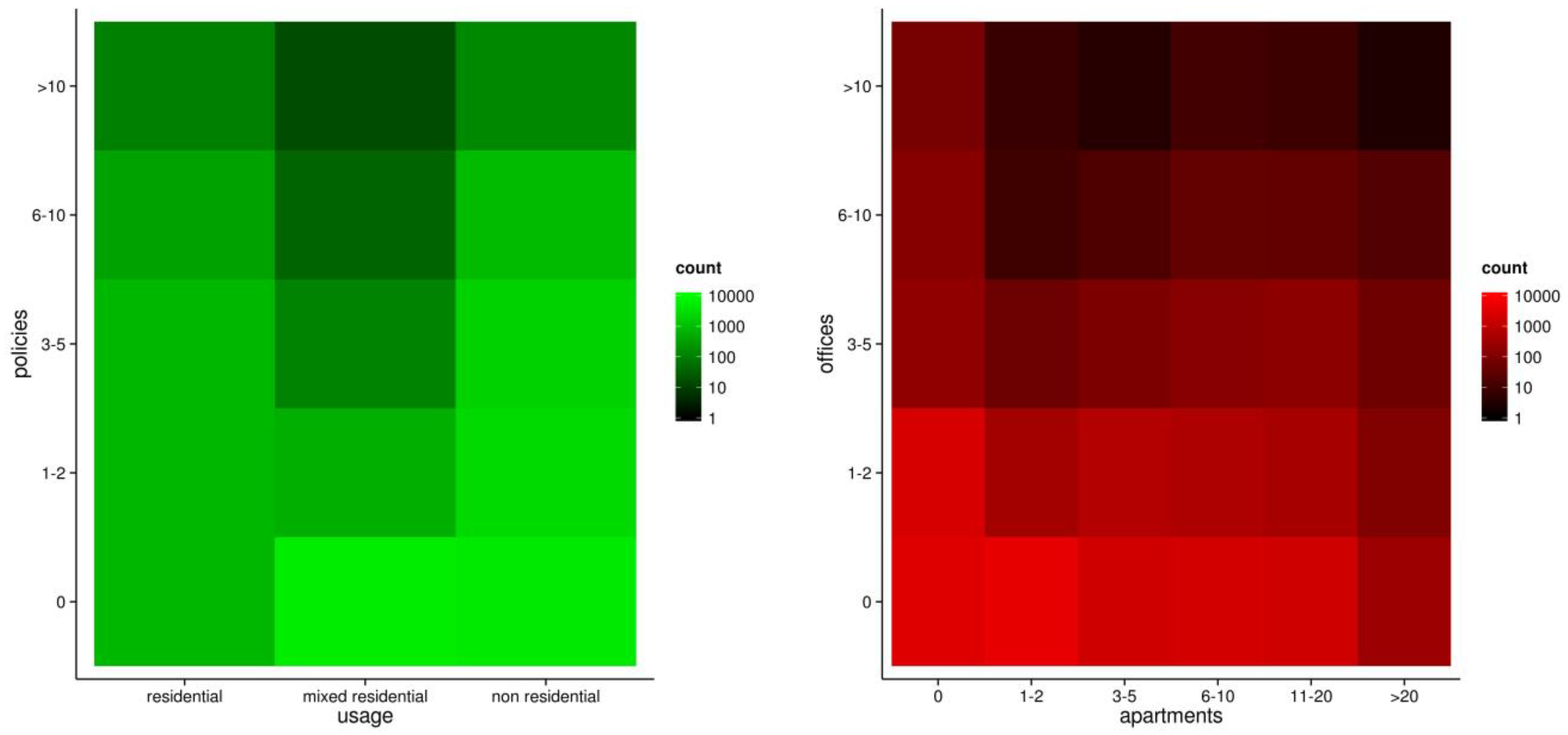
Figure 5. Composition of the training dataset of 1000 buildings randomly selected among the 19,158 buildings of the original dataset (“count” refers to the number of TCIP policies in the building).

Figure 5. Composition of the training dataset of 1000 buildings randomly selected among the 19,158 buildings of the original dataset (“count” refers to the number of TCIP policies in the building).

This type of information is available at very high resolution in Istanbul as well as in other large settlements in Turkey, and the trend is expected to improve in the next years. In order to simulate a “data-poor” case, where only limited information is available for making inferences, 1000 buildings were randomly sampled from the original population of 19,158 available in Besiktas (5.2% of the overall population). The selected buildings covered 1523 policies, with a relative distribution in terms of usage, apartments, and offices depicted in Figure 5.

The selected data and used to train a logistical regression engine, whose functional form is:

$$p\left(p{n}_i\right)~{\beta }_0+{\displaystyle \sum {\beta }_j}\ast att{r}_j$$

(1)

where p(pn_i) represents the probability of finding in a building a number of policies belonging to the interval i, and β_j is the regression coefficient of attribute j. The considered attributes (available for the buildings sampled) are listed in Table 1. The variable encoding the number of policies has been subdivided into five intervals, shown in Table 2.

Table 1. Attributes used to constrain the logistic regression.

Attribute		Description
1	stories	Number of stories, including mansard and basement
2	constr	Type of construction (eight different types were listed)
3	usage	Type of usage (residential, mixed residential, non-residential)
4	apartments	Number of apartments
5	offices	Number of offices
6	carparks	Number of parking lots

Table 1. Attributes used to constrain the logistic regression.

Attribute		Description
1	stories	Number of stories, including mansard and basement
2	constr	Type of construction (eight different types were listed)
3	usage	Type of usage (residential, mixed residential, non-residential)
4	apartments	Number of apartments
5	offices	Number of offices
6	carparks	Number of parking lots

Table 2. Confusion matrix comparing predicted and observed number of policies for a 10,000 test dataset in Besiktas.

Predict./Observ.	0	1–2	3–5	6–10	>10
0	5266	1376	358	53	7
1–2	150	298	225	33	4
3–5	177	425	835	381	22
6–10	20	23	54	127	31
>10	8	2	11	50	64

Table 2. Confusion matrix comparing predicted and observed number of policies for a 10,000 test dataset in Besiktas.

Predict./Observ.	0	1–2	3–5	6–10	>10
0	5266	1376	358	53	7
1–2	150	298	225	33	4
3–5	177	425	835	381	22
6–10	20	23	54	127	31
>10	8	2	11	50	64

From the analysis of the coefficients computed by the regression, it can be noted that the variables stories, apartments, and offices show a positive correlation with the number of policies, while the variables usage (mixed residential) and carparks show a negative correlation, relatively strong for the usage type ‘mixed residential’. The number of policies obtained by the computed regression has been compared with the observed ones for a further dataset of 10,000 buildings uncorrelated with the one used for training. The regression algorithm provides for each tested building the probability of finding a number of policies within one of five intervals: 0, 1–2, 3–5, 6–10, and >10. These probabilities can be aggregated to compute a single scalar index that represents the “susceptibility” of the considered buildings to host earthquake insurance policies (see Equation (2)):

$$index=\frac{\text{1}}{\text{5}}{\displaystyle \sum i}\ast p_i$$

(2)

The confusion matrix of the comparison is shown in Table 2. The table shows that the logistic regression is able to capture the general correlation trend between the considered attributes and the number of policies, but cannot precisely infer the particular interval. On the one hand, this can be due to the natural bias of the training and test set, since buildings that are good candidates for having policies have not necessarily already been reached by TCIP, which had a penetration close to 40% in the town when these data were released.

A more thorough exploration of different predictive approaches would definitely improve the performance of the inference process. It is also important to note that in order for the predictive sampling to be useful, it has to capture the general correlation trend in order to further optimize the computation of the focus maps and thus the field survey.

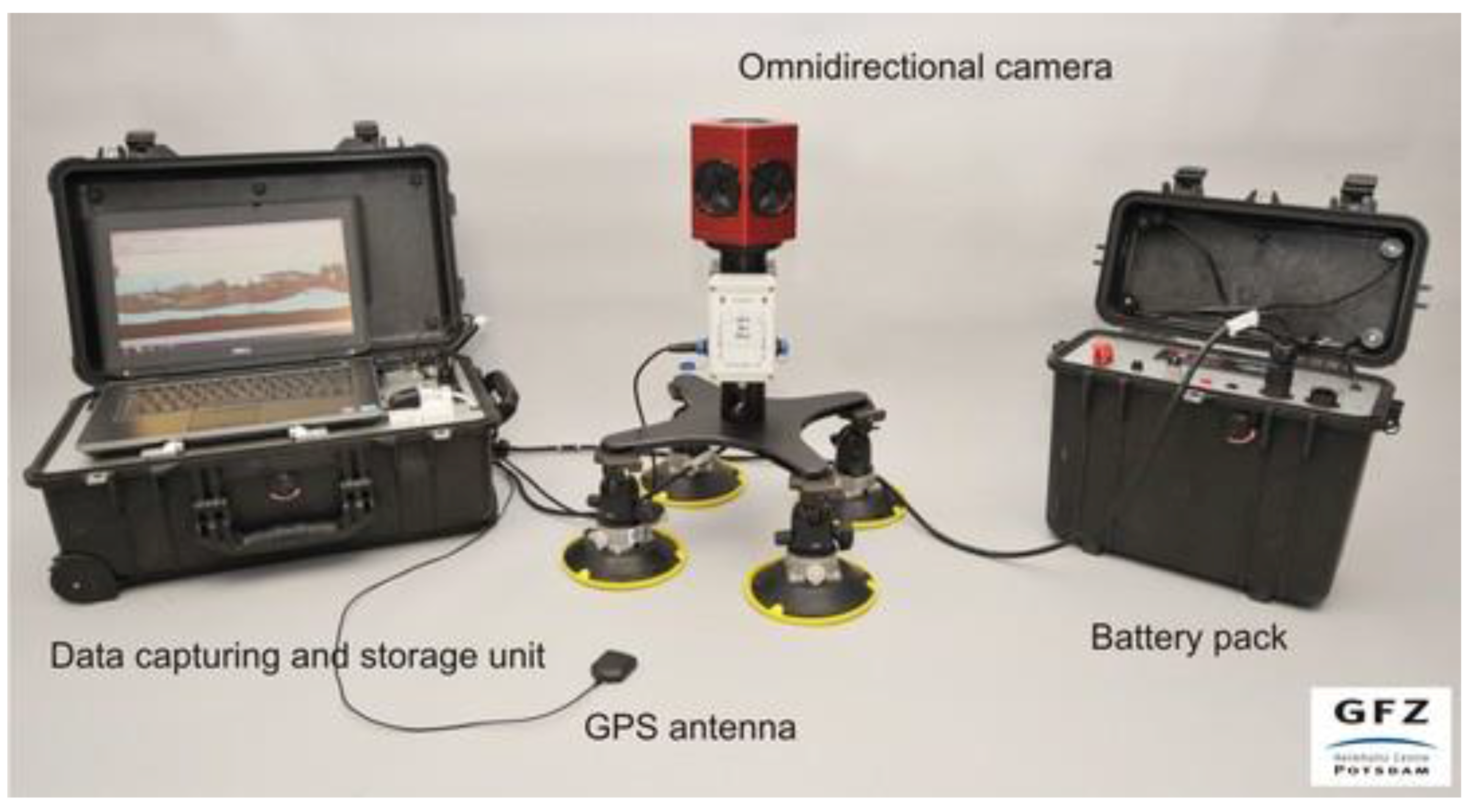
4. Mobile Mapping

For rapid in situ image data capturing, a mobile mapping system (GFZ-MOMA) has been developed and extensively tested [25,26]. The system is composed of a Ladybug3 omnidirectional camera from Point Grey Research Ltd., a data capturing and storage unit, a navigation unit, and an external battery pack that supplies the energy for up to 6 h of autonomous operation (Figure 6).

The Ladybug3 (See http://www.ptgrey.com/ for full technical specifications) camera is made up of six color Complementary Metal Oxide Semiconductor (CMOS) sensors that capture concurrent image sequences with an acquisition rate of up to 15 fps (frames per second). The six single-camera image streams are synchronized and automatically stitched into an omnidirectional (panoramic) high resolution (5700 × 2700 px) format with JPEG compression. The camera system is operated from inside the car and is mounted on the vehicle’s roof with a simple mounting system composed of a light-weight aluminum frame and four high-power suction cups.

Figure 6. GFZ-MOMA omnidirectional mobile mapping system with data capturing and storage unit, and battery pack.

Figure 6. GFZ-MOMA omnidirectional mobile mapping system with data capturing and storage unit, and battery pack.

The data capturing and storage unit has been developed with a specific focus on ease of use and ruggedness for robust outdoor applications, even under rough conditions (e.g., unpaved roads, dust). The main component of the unit is a standard notebook with a 750GB Serial ATA hard drive. A commercial-grade GPS receiver provides geo-localization with a 1 Hz epoch rate. An optional Inertial Measurement Unit (IMU) can be used to record additional data about the 3D camera pose. The notebook and all the other components are fixed into a rugged hard plastic case. A custom-designed software application captures, synchronizes, and saves the different data streams coming from the camera, the GPS, and the IMU. The synchronization of the data, within 125 ms, is based on the timer embedded in the ieee-1394B hardware controller. Location is associated with each omnidirectional image by b-spline interpolation of GPS positioning.

The navigation unit uses QGIS, a free, open-source GIS environment, as the main software component for location tracking and car navigation. Its map interface is able to combine various background maps of the study area and to display pre-calculated sample areas and routes. The position can be tracked and displayed in real time with the GPS live tracking functionality. This allows an operator to not only navigate the car along pre-calculated routes, but also to reschedule the path on-the-fly to cope with unexpected environmental conditions (e.g., traffic jams or road blockages).

5. Results

5.1. Survey Design

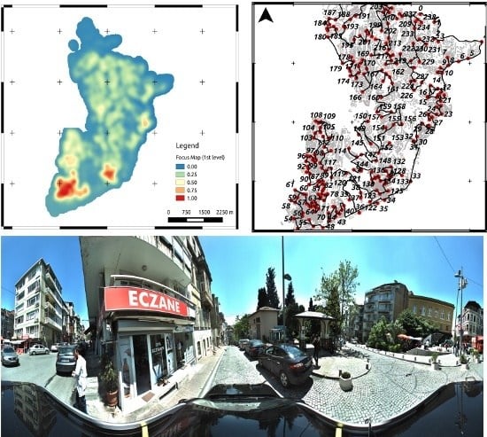
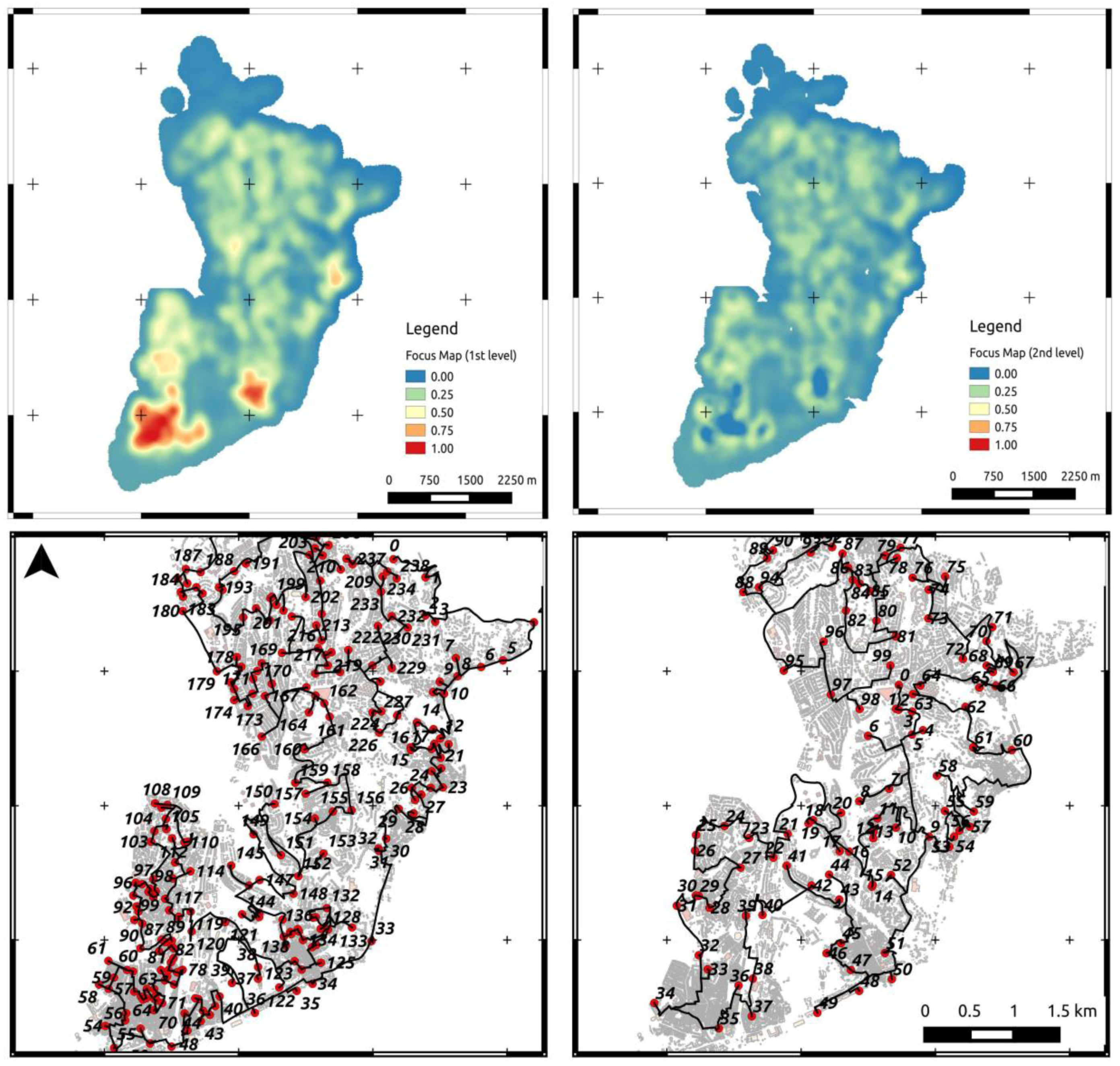
The purpose of the overall approach is to efficiently collect visual data on possibly damaged buildings in a realistic urban environment. A full scale test in a post-earthquake situation has not yet been possible, hence in order to evaluate the expected performance of the system in a realistic environment a pre-event data collection has been carried out in the study area. The survey has been designed with a two-stage format, with iterative sampling and routing. A focus map was generated as described in Section 3 with a linear (additive) pooling approach in order to widen the range of the survey, since it was mostly considered a pre-event one. The resulting focus map for the first acquisition day is presented in Figure 7.

In our case the following datasets have been used:

• distribution of buildings, also accounting for the density of policies (number of policies per building),
• hazard map in terms of expected PGV with exceedance probability of 10% in 50 years.

The latter represents a proxy for the expected location of building damage, in the absence of a particular scenario, while the first dataset encodes both the spatial distribution of buildings and the co-variant distribution of policies. Layers have been normalized with a standard linear approach, using (1%, 99%) rejection bounds (see [11] for details on available normalization techniques).

Figure 7. Computation of pre-event focus map. (A) spatial distribution of buildings weighted with related number of earthquake policies. (B) expected seismic hazard (PGA) with exceedance probability of 10% in 50 years. (C) resulting focus map obtained by linear pooling of the normalized layers with weights (0.7,0.3).

Figure 7. Computation of pre-event focus map. (A) spatial distribution of buildings weighted with related number of earthquake policies. (B) expected seismic hazard (PGA) with exceedance probability of 10% in 50 years. (C) resulting focus map obtained by linear pooling of the normalized layers with weights (0.7,0.3).

The two layers have been assigned respective weights (0.7, 0.3), therefore giving priority to the location of policies, but also taking into account the expected hazard (hence the expected damage). A second-level focus map has been computed considering as the additional layer a polygon around the geometrical path obtained from the first focus map, and considered using a negative weight in the pooling phase. Two sampling sets have then been generated with a PPS sampling scheme (see Section 3 and [11,12]). The two focus maps and the related optimized routes are shown in Figure 7. As can be seen from the figure, the optimized paths for a two-day multi-stage survey provide a good coverage of the areas where the focus maps have higher values, with a small amount of superposition. The routing of the second day not only follows the underlying focus map, but also considers the previously captured route. Table 3 lists the main geometric features of the two individual surveys. The overall distance expected to be traveled is around 145 km. In normal conditions (in urban environments) a mobile mapping system can cover between 80 and 120 km within a 6–8 h time span. The first day survey is along this line, while the survey on the second day is shorter, and can be thought of as a refinement survey.

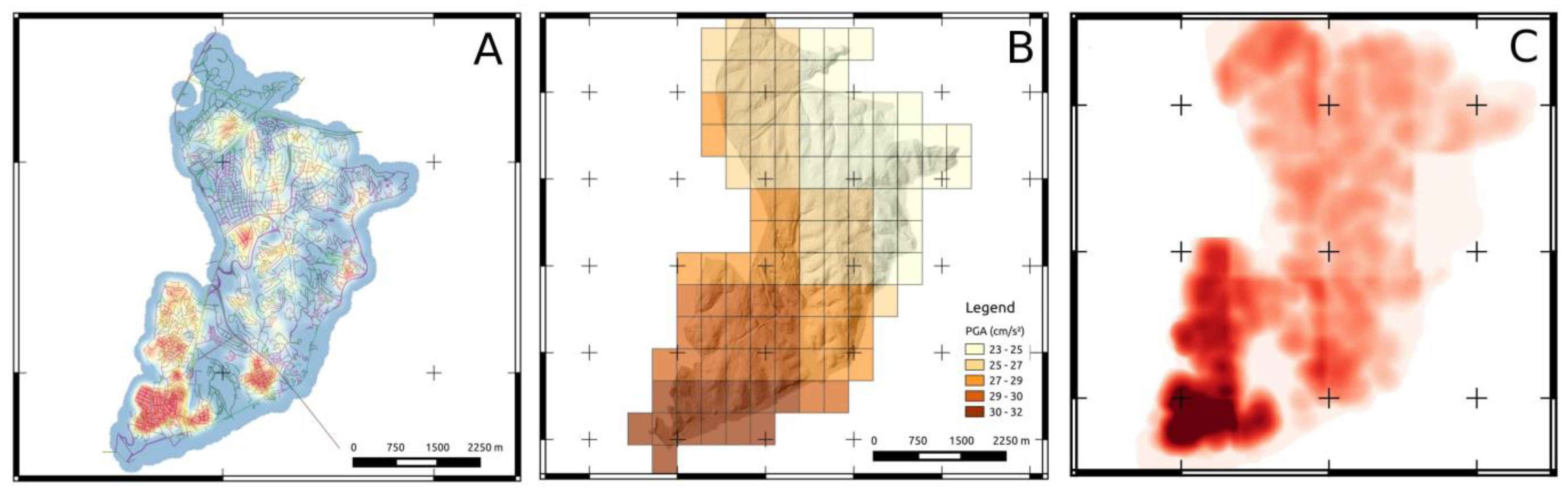
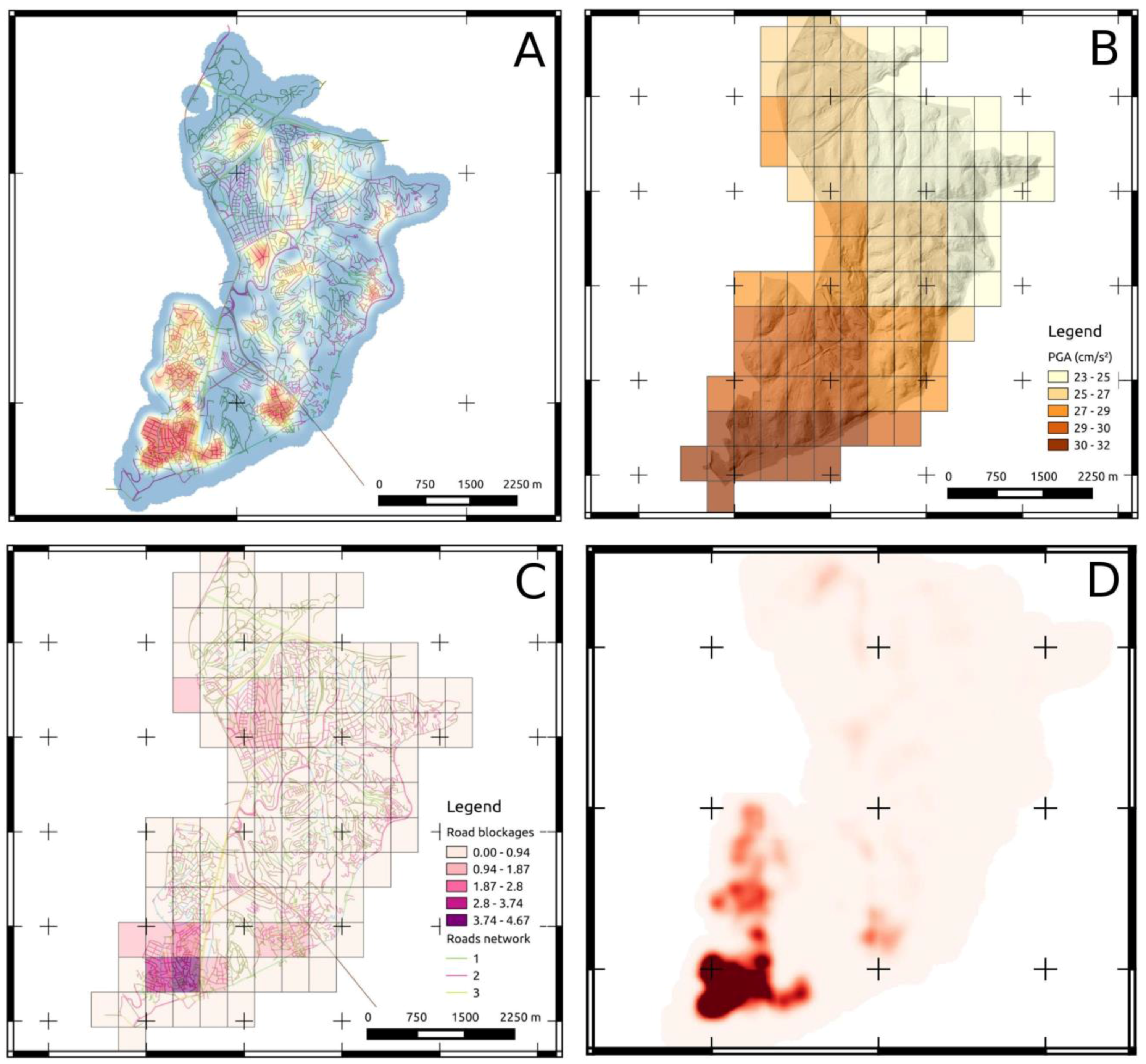
A simulation of a post-event survey has also been performed using the available data. A focus map (see Figure 8D) based on log-linear (multiplicative) pooling is suggested in this case , since a higher level of selectivity should be sought in order to optimize the survey efforts. In order to simulate a more realistic case, the basic layers used in the pre-event case (distribution of buildings/policies and seismic hazard) have been considered. A further layer describing the expected spatial distribution of road blockages has been added (displayed in Figure 8C). This can be further integrated, in a real case, by either the expected damage distribution from satellite/aerial observations, or by in situ information provided by local authorities. This information can moreover be used to constrain the path optimization, for instance by assigning a higher cost to route segments of reduced width (e.g., small lateral roads frequent in the Besiktas district) in areas subject to collapses, which would be more prone to blockage due to debris.

Table 3. Summary of 2-stage survey designed for Besiktas district.

Survey Stage	Route Length (km)	No. of Route Points	No. of Road Segments
1st day	82.6	238	1287
2nd day	64.1	99	903

Table 3. Summary of 2-stage survey designed for Besiktas district.

Survey Stage	Route Length (km)	No. of Route Points	No. of Road Segments
1st day	82.6	238	1287
2nd day	64.1	99	903

Figure 8. Computation of post-event focus map. (A) spatial distribution of buildings weighted with related number of earthquake policies. (B) expected seismic hazard (PGA) with exceedance probability of 10% in 50 years. (C) expected spatial distribution of road blockages. (D) resulting focus map obtained by log-linear pooling of the normalized layers.

Figure 8. Computation of post-event focus map. (A) spatial distribution of buildings weighted with related number of earthquake policies. (B) expected seismic hazard (PGA) with exceedance probability of 10% in 50 years. (C) expected spatial distribution of road blockages. (D) resulting focus map obtained by log-linear pooling of the normalized layers.

In order to implement the actual survey, a sample set has to be generated after the pre-event focus map and subsequently routed. The optimized routes for a two-day survey are displayed in Figure 9. The expected linear distances covered by the computed paths are listed in Table 3. Based on these routes, the mobile mapping system described in Section 4 has been deployed in the field and operated. In the next sections, the results of the field activities are discussed.

Figure 9. Iterative, multi-stage sampling and routing for a two-day survey. The upper row shows the computed first-level focus map (left) and the second-level focus map (right) obtained by considering the first-level focus map as additional (negatively weighted) layer. The lower row shows the optimized routing for the first day and second day, under consideration of the first day’s route.

Figure 9. Iterative, multi-stage sampling and routing for a two-day survey. The upper row shows the computed first-level focus map (left) and the second-level focus map (right) obtained by considering the first-level focus map as additional (negatively weighted) layer. The lower row shows the optimized routing for the first day and second day, under consideration of the first day’s route.

5.2. Survey Length and Speed

The lengths of the actual surveys are listed in Table 4. In total, around 120 km have been driven in approximately 10 h, split between two days. As can be noted by comparing Table 3 and Table 4, the paths followed by the mobile mapping system are slightly different from the optimized routes. The most common reasons for deviating from the original routes include inconsistencies in the routing due to a lack of information about the road networks (information about one-way streets was not available) or accessibility issues related to unexpected road blockages.

Table 4. Summary of the two-day survey conducted in Besiktas.

Survey Stage	Distance Covered (km)	Elapsed Time (h)	Buildings Covered (Viewshed)	% of the Total Buildings	Policies Covered (Viewshed)	% of the Total Policies
day-1	72.5	6	4922	25.7	9327	31.2
day-2	45.9	4	2270	11.8	3812	12.8
totals	118.4	10	7192	37.5	19,945	44.8

Table 4. Summary of the two-day survey conducted in Besiktas.

Survey Stage	Distance Covered (km)	Elapsed Time (h)	Buildings Covered (Viewshed)	% of the Total Buildings	Policies Covered (Viewshed)	% of the Total Policies
day-1	72.5	6	4922	25.7	9327	31.2
day-2	45.9	4	2270	11.8	3812	12.8
totals	118.4	10	7192	37.5	19,945	44.8

In Figure 10 the speed of the car carrying the mobile mapping system during the survey is shown. The average speed over the two-day survey is about 12 km/h, but there are a number of locations where the speed dropped to around 5 km/h. This is mostly due to the complex nature of the selected district, with very narrow streets (sometimes only a few cm larger than the car) often crowded by people and commercial vehicles.

Figure 10. The color of the trace is proportional to the absolute speed of the mobile mapping system (left). Distribution of the speed during the survey (logarithmic scale) in Km/h (right).

Figure 10. The color of the trace is proportional to the absolute speed of the mobile mapping system (left). Distribution of the speed during the survey (logarithmic scale) in Km/h (right).

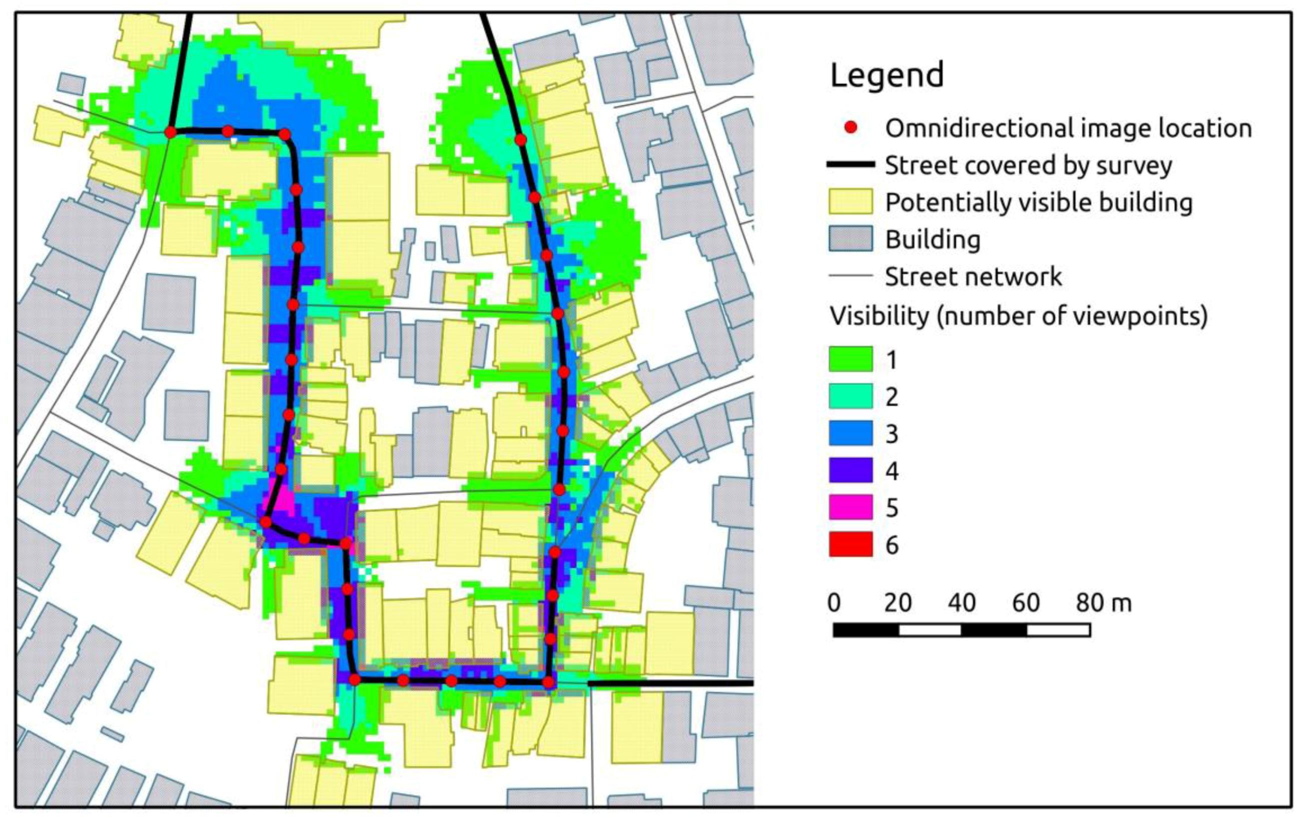
5.3. Survey Coverage

In order to evaluate the performance of the system with respect to its intended scope, which is the collection of visual information on the built-up environment, a visibility analysis has been conducted on the collected data. The purpose of the analysis was to assess the expected coverage in terms of buildings and policies, and to highlight possible issues connected with the use of the proposed mobile mapping system. A cumulative viewshed analysis [27] along the path followed by the mobile mapping system has been carried out to select all buildings that are potentially visible from the acquired image locations (Figure 11). The algorithm iteratively loops through a set of input points and calculates viewshed maps, which depict the geographical area that is visible from the input point given digital elevation information. As input elevation information, the DSM of the study area has been used, observer points have been set along the survey path at 3 m above ground (the actual height of the omnidirectional camera mounted on the car) with an equal spacing of 20 m and a maximum viewing distance of 30 m. The output is a cumulative viewshed map with raster cells being assigned the number of input locations that have visibility. A spatial intersection with the building footprints provides an estimate of the buildings that are potentially visible from the surveyed path. The estimated number of buildings covered by the survey and the related number of policies involved are presented in Table 4. Based on the viewshed analysis, it is estimated that more than 7000 buildings, equating to almost 20,000 policies, have been captured by the mobile mapping system. This equals 37.5% of the total building stock and 44% of the total number of policies in the study area.

In order to further analyze the visibility under consideration of occlusion factors that could not be considered in the viewshed analysis (e.g., vegetation, cars, walls, etc.), a set of 1000 buildings has been randomly sampled from the ones identified as being potentially visible by the viewshed analysis. An operator has been asked to manually locate the selected buildings in the omnidirectional stream, and to assess whether they are actually visible (at least partly) or hidden. The operator had to report the type of occlusion, even when the selected building was considered visible for the purpose of the survey, and to write down any other issues related to the requested analysis. At least 50% of a building should be visible in order to be assigned the label visible. A Remote Rapid Visual Screening (RRVS) desktop environment has been set up to perform the image analysis, as is described in [28]. In Table 5 the results of the detailed occlusion analysis are reported.

Figure 11. Visibility analysis based on viewshed estimation for a subset of the buildings theoretically imaged by the mobile mapping system.

Figure 11. Visibility analysis based on viewshed estimation for a subset of the buildings theoretically imaged by the mobile mapping system.

The operator was a university student with experience in remote sensing and desktop mapping. The desktop assessment was carried out in one week, considering an average of 5–6 h a day. In the practical application, different operator profiles could be employed to fulfill different tasks. For instance, non-skilled operators could be employed for a very quick screening of the captured data (e.g., subdividing damaged building into very coarse categories), while trained engineers, architects, and claim adjusters would be dedicated to a more detailed analysis of the collected information.

Out of all the analyzed buildings, 79% are visible or partly visible, while around 21% are not visible. Among the visible ones, the most frequent occlusion is represented by other buildings, followed by vegetation (mostly trees). Interestingly, the most frequent cause of total occlusion is vegetation, but a significant portion (34% in the specific test) is connected to a number of different, often temporary causes, for instance other vehicles passing by, or advertisements.

Table 5. Results of occlusion analysis performed on a random sampling of 996 buildings within the viewshed around the survey path.

Occlusion Type	Visible			Not Visible
	Counts	% of Total Samples	% of Total Visible	Counts	% of Total Samples	% of Total Non-Visible
Other buildings	532	53.2	67.2	14	1.4	6.7
Vegetation	170	17.0	21.5	72	7.2	34.5
Walls, fences	33	3.3	4.2	33	3.3	15.7
Other occlusions	49	4.9	6.2	70	7.0	33.5
Unspecified	7	0.7	0.9	20	2.0	9.6
total	791	79.5	-	209	20.5	-

Table 5. Results of occlusion analysis performed on a random sampling of 996 buildings within the viewshed around the survey path.

Occlusion Type	Visible			Not Visible
	Counts	% of Total Samples	% of Total Visible	Counts	% of Total Samples	% of Total Non-Visible
Other buildings	532	53.2	67.2	14	1.4	6.7
Vegetation	170	17.0	21.5	72	7.2	34.5
Walls, fences	33	3.3	4.2	33	3.3	15.7
Other occlusions	49	4.9	6.2	70	7.0	33.5
Unspecified	7	0.7	0.9	20	2.0	9.6
total	791	79.5	-	209	20.5	-

5.4. GPS Positioning Accuracy

Although in general the positioning accuracy of the mobile mapping system is adequate for the considered task (ranging from 2 to 5 m), in several cases the system experienced problems in the geo-referencing of the images due to poor GPS signal reception. This problem, particularly present in the areas with a higher density of buildings and the presence of “urban canyons,” caused the misplacement of the survey path, with positioning errors ranging from a few meters to more than 30 m. Since this can affect the correct identification of the targeted building, in the offline analysis phase the operator was asked to evaluate whether the inconsistencies in the positioning would seriously hinder the analysis procedure itself. It has been noticed that, out of 1000 considered buildings, in around 120 cases (~12%) the image coordinates appeared misplaced (by visual judgment by the operator). In most of the cases the operator was still able to locate the targeted building despite the geo-referencing error. In 45 cases the operator could not retrieve the building in the exam, thus declaring the building as non-visible. Even though the impact of this issue in the preliminary testing was limited, affecting ~4.5% of the samples, the technological issue has to be addressed in the operational phase.

5.5. Image Quality

An example of the images collected during the survey is provided in Figure 12. The images were collected at approximately 6 fps, and a total of around 700 GB data was collected during the two-day survey. The omnidirectional images are obtained by dynamic stitching of the raw video-streams captured by the six individual cameras. The resulting image has a field of view of 360° horizontally and about 170° vertically, with a resolution of about 12 mega-pixels. An example is shown in Figure 13. The quality of the images, assessed during the visibility analysis described in the preceding section, has been deemed adequate for the purpose of the system, which is the rapid assessment of medium to extensive damage. The resolution of the images allows for the detection of features described in Figure 12. Moreover, the panoramic format of the images allows for an intuitive and thorough analysis of the built-up environment, particularly suitable in the narrow streets characterizing the selected district.

The shutter of the system is automatically managed by the camera system’s software, and is continuously updated in order to obtain a balanced appearance of the image in the presence of strong brightness differences. This allows the system to promptly compensate for abrupt changes in the ambient illumination. This is exemplified by comparing the images in Figure 13A and Figure 13B. The two images have been taken from almost the same vantage point during two surveys, with the illumination conditions being dramatically different in the two images. Nonetheless, even the picture taken during dark and rainy conditions was suitable for a building assessment.

Figure 12. Example of an omnidirectional image showing a (non-structural) damage of a building. The distance between building and camera is of about 20 m. The damage is visible in the lower part of the image, circled in yellow. The upper right inset shows the geographical location of the captured omnidirectional image.

Figure 12. Example of an omnidirectional image showing a (non-structural) damage of a building. The distance between building and camera is of about 20 m. The damage is visible in the lower part of the image, circled in yellow. The upper right inset shows the geographical location of the captured omnidirectional image.

Figure 13. Upper section: example of omnidirectional image. Lower section: (A) Partial rectilinear re-projection of the omnidirectional image. Only a portion of the original image is visible, but the operator can dynamically change the angle of view, direction, and apparent zoom in the re-projected image. (B) Rectilinear projection of an omnidirectional image taken in the sample place at a different time, and with rainy weather.

Figure 13. Upper section: example of omnidirectional image. Lower section: (A) Partial rectilinear re-projection of the omnidirectional image. Only a portion of the original image is visible, but the operator can dynamically change the angle of view, direction, and apparent zoom in the re-projected image. (B) Rectilinear projection of an omnidirectional image taken in the sample place at a different time, and with rainy weather.

5.6. Dependency on Sampling and Routing

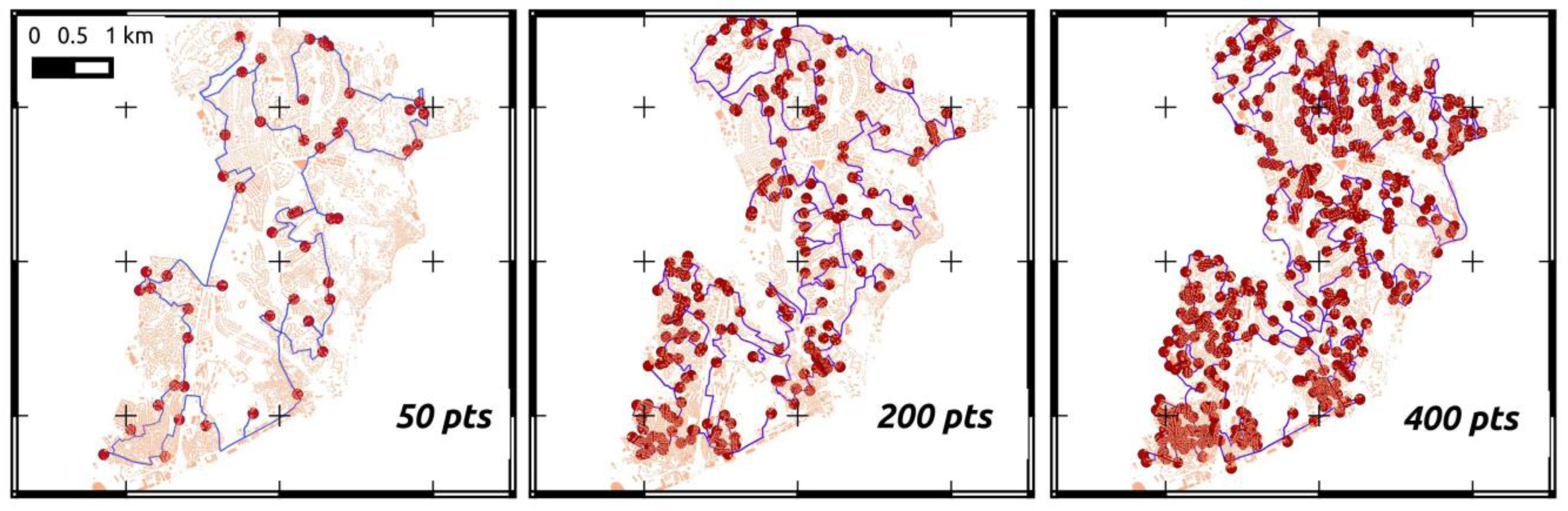
Within a single-stage survey, a parameter directly affecting the resulting survey design is the number of points used to generate the sampling set. A test has been conducted in order to assess how the size of the sampling set is related to the extent and coverage of the resulting survey. This can be used to tune the survey length independently on the focus map driving the spatial prioritization.

Four different surveys have been generated for four different sampling sets, respectively containing 50, 100, 200, and 400 points (referred to as the sample size, sd). Each sampling set has been generated after the same focus map and following the same PPS sampling design (see Figure 14).

Figure 14. Comparison among different single stage surveys based on different sample sets. From the left, results are shown for 50-, 200-, and 400-point sample sets.

Figure 14. Comparison among different single stage surveys based on different sample sets. From the left, results are shown for 50-, 200-, and 400-point sample sets.

Figure 15. Comparison between the length of the resulting route in the optimized case (blue plot) and in the random case (black plot with red points) (top). As the plot shows, the route length is proportional to the square root of the dimension of the sample set, and the random route is systematically longer. Comparison of the expected number of covered policies with respect to route length (in km) for random sampling (black line, red dots) and focused sampling (blue line, blue dots) (bottom). The relationship is apparently linear for the focused sampling, while it appears to not be linear for the random sampling, which is much less efficient in any case.

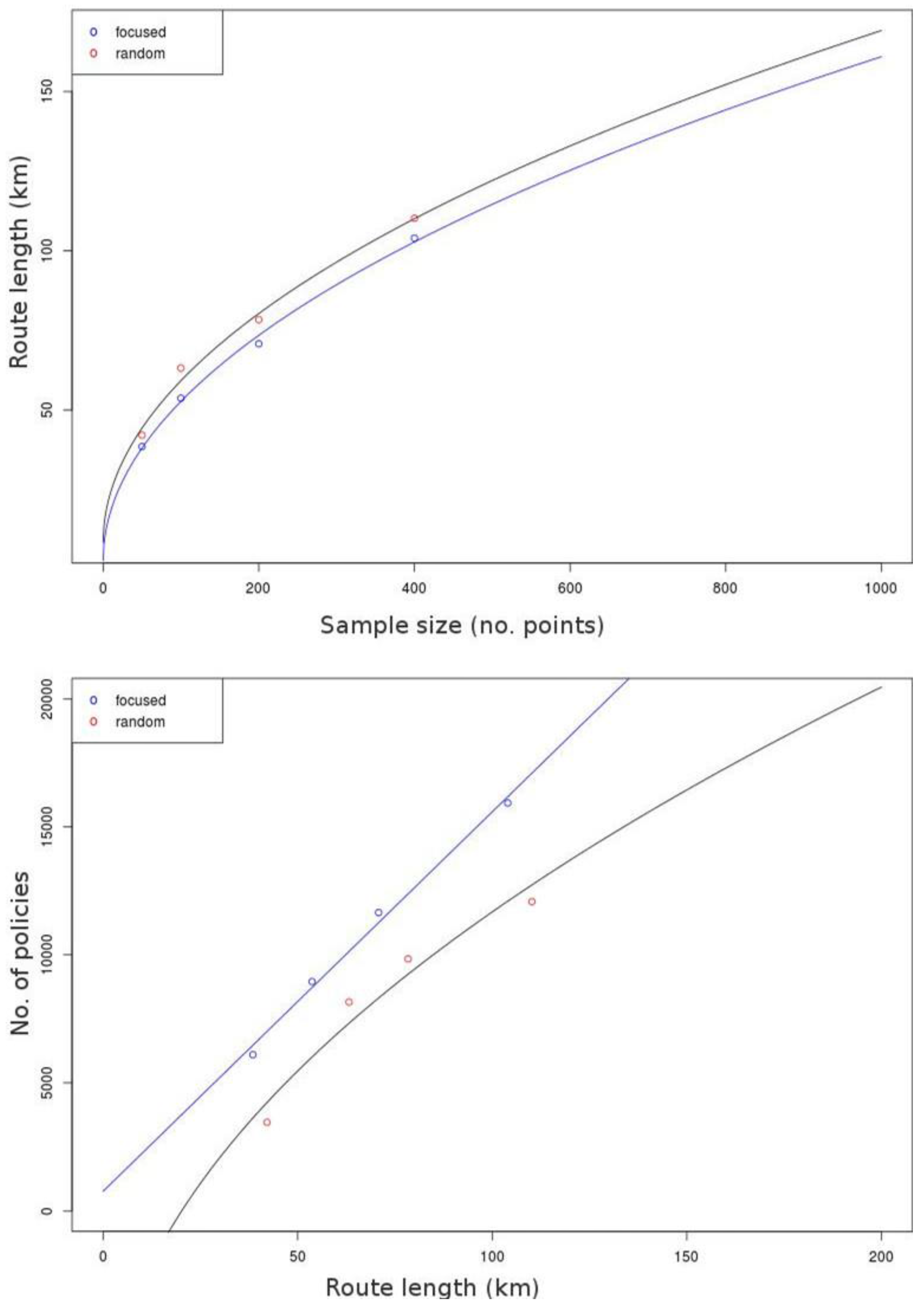
Figure 15. Comparison between the length of the resulting route in the optimized case (blue plot) and in the random case (black plot with red points) (top). As the plot shows, the route length is proportional to the square root of the dimension of the sample set, and the random route is systematically longer. Comparison of the expected number of covered policies with respect to route length (in km) for random sampling (black line, red dots) and focused sampling (blue line, blue dots) (bottom). The relationship is apparently linear for the focused sampling, while it appears to not be linear for the random sampling, which is much less efficient in any case.

Table 6. Empirical correlation between dimension of the sample sets, length of the resulting survey (in km), and number of covered buildings (i.e., lying within a 30-m buffer from the driven route).

Sample Set sd (No. of pts)	Survey Length L (km)	% of Street Network	Covered Buildings (30 m Buffer)	% of Building Stock
50	38.5	10	3629	19
100	53.7	14	5279	28
200	70	18.3	6414	33.5
400	104	27	8567	44.8

Table 6. Empirical correlation between dimension of the sample sets, length of the resulting survey (in km), and number of covered buildings (i.e., lying within a 30-m buffer from the driven route).

Sample Set sd (No. of pts)	Survey Length L (km)	% of Street Network	Covered Buildings (30 m Buffer)	% of Building Stock
50	38.5	10	3629	19
100	53.7	14	5279	28
200	70	18.3	6414	33.5
400	104	27	8567	44.8

In Table 6 the empirical correlation between the dimension of the sample set and the length in km of the resulting survey is reported. As displayed by the graph in Figure 15 (top), the length L of the resulting route is proportional to the square root of the sample size sd:

$$L={\alpha }_0+{\alpha }_1\sqrt{sd}$$

(3)

where the fitted coefficients α₀ = −0.7561 and α₁ = 5.1925, and the r-squared value is 0.9972.

Since, depending on the selected location, the average speed of the mobile mapping system can be estimated, knowledge of the relationships between sampling set and survey length allows for more efficient preparation of field activities.

5.7. Focused Survey vs. Random Survey

In order to understand the actual impact of the optimization approach proposed to implement ground-based surveys, a comparison has been made with a survey based on a random sampling of the selected area in Besiktas.

In addition to the sampling sets generated after a focus map, as described in the preceding section, and hereby defined as “focused,” a parallel set of points, referred to as “random,” has been generated using a simple random sampling scheme (corresponding to using a uniform focus map on the selected area). The random set has been automatically routed using the same approach as the focused one, and the resulting routes have been analyzed by estimating the number of buildings and the number of related policies expected to be covered during the surveys. The number of covered buildings, i.e., the buildings that can be visually inspected based on the performed survey, is approximated by the number of the buildings lying inside a 30-m buffer around the computed route. The number of covered policies is therefore simply the sum of the insurance policies associated with the covered buildings. In Table 7 a comparison is provided of the two approaches. The difference between the computed estimates in the two cases, expressed as percentages in Table 7, is defined in Equation (4):

$$dif=\text{2}\frac{\left(focused-random\right)}{\left(focused+random\right)}$$

(4)

Table 7. Comparison between routing based on random sampling and routing based on focused sampling.

Sample Points	Route Length (km)			Covered Buildings (30-m Buffer)			Covered Policies (30-m Buffer)
	Focus	Rand	% Diff	Focus	Rand	% Diff	Focus	Rand	% Diff
50	38.5	42.1	−9%	3629	2128	70%	6098	3460	76%
100	53.7	63.2	−16%	5279	4685	13%	8955	8161	10%
200	70.8	78.3	−10%	6414	5820	10%	11652	9843	18%
400	104	110.2	−6%	8567	6980	23%	15935	12082	32%

Table 7. Comparison between routing based on random sampling and routing based on focused sampling.

Sample Points	Route Length (km)			Covered Buildings (30-m Buffer)			Covered Policies (30-m Buffer)
	Focus	Rand	% Diff	Focus	Rand	% Diff	Focus	Rand	% Diff
50	38.5	42.1	−9%	3629	2128	70%	6098	3460	76%
100	53.7	63.2	−16%	5279	4685	13%	8955	8161	10%
200	70.8	78.3	−10%	6414	5820	10%	11652	9843	18%
400	104	110.2	−6%	8567	6980	23%	15935	12082	32%

6. Discussion

The preliminary test presented in the last section shows the empirical relation between the size of the sampling set based on the reference focus map, the overall length of the survey (in km), and the expected visual coverage in terms of buildings and, more importantly in this application, earthquake insurance policies. By developing such empirical models, a complete optimization and tuning of the field surveys is possible, accounting both for the users’ priorities encoded into the focus map and the constraints related to available resources and environmental conditions.

Looking at the values in Table 7 and the plots in Figure 15, it can be noted that the “focused” sampling is consistently more efficient than the “random” sampling; in the latter case, the route length, for instance, is on average longer.

Under the same conditions, the focused survey was able to systematically capture more buildings with respect to a random survey. Even stronger is the comparison between the policy coverage.

The focused survey therefore always outperformed the random survey in the considered tests. We have to stress that these are preliminary evaluations, based on a small number of realizations (four realizations related to different sampling sets). More thorough testing should be undertaken (and is envisaged), but the current outcomes already provide an indication of the potential of the proposed approach. These results are not surprising, considering that the computed focus map increases the inclusion probability of the locations with higher density of buildings and policies.

The relationship between the route length and the number of the covered policies is expected to be linear in the focused case using a PPS sampling scheme (since is linearly depending on the density of buildings and policies, which we suppose as roughly constant). This is easily verified and is visible in Figure 15 (lower).

7. Conclusions

A widespread earthquake insurance scheme is recognized as a powerful tool to share the economic risk resulting from low-probability, high-impact seismic events, at the same time boosting the subsequent recovery stage. The more swift and fair the settling of claims after an earthquake, the quicker the kick-start of the impacted communities, and the greater the overall resilience of the affected country. Unfortunately, claim management is a complex process that does not always scale smoothly with the number of the filed claims, and in the occurrence of a major event in areas with high vulnerability and high policy density, a substantial number of claims can be expected. This occurrence could overwhelm the operational structure of the Turkish Catastrophe Insurance Pool (TCIP), which in Turkey is providing country-wide earthquake insurance with a significant penetration rate.

A prompt and efficient visual survey of the insured (possibly damaged) building stock would significantly enhance the operational capabilities of the TCIP in the aftermath of a powerful earthquake in Istanbul. An innovative solution has been proposed based on the deployment of an agile mobile mapping system whose field operations are optimized through a geo-statistical approach.

In order to test the proposed approach, a field test has been carried out in Besiktas, Istanbul. The selected district encompasses different characteristics that are common to other locations in the town, hence providing a significant example of the environmental conditions to be expected on a wider geographic scale.

This preliminary assessment shows how a careful optimization of the sampling and routing protocols can yield much better results than a simple random survey. In a similar way to pre-event surveys, a focus map has to first be evaluated in order to optimize the actual post-event survey. Several datasets and ancillary information can be used, including:

• distribution or density of buildings;
• distribution or density of policies;
• expected damage (based on pre-computed scenarios);
• damage information based on rapid assessment through remote sensing or aerial/UAV surveys;
• observed damage based on field assessment or reports from civil protection authorities.

Other information, such as for instance the assessment of road blockage due to debris and/or to search and rescue activities, the probability of fire following earthquake, liquefaction hotspots, and landslide information, can also be included in the focus map, or can be used as additional penalty terms in the routing phase.

Significant advancement of claim management could be obtained by applying the proposed method on a large scale. In the Istanbul case, any possible means of optimizing claim management must be pursued in order to improve the resilience of the community. Further tests are due, but the preliminary results are promising. We recommend that TCIP implement and embed the proposed approach in the complex operational structure that steers the management of claims.