Inferring Directed Road Networks from GPS Traces by Track Alignment

Abstract

This paper proposes a method to infer road networks from GPS traces. These networks include intersections between roads, the connectivity between the intersections and the possible traffic directions between directly-connected intersections. These intersections are localized by detecting and clustering turning points, which are locations where the moving direction changes on GPS traces. We infer the structure of road networks by segmenting all of the GPS traces to identify these intersections. We can then form both a connectivity matrix of the intersections and a small representative GPS track for each road segment. The road segment between each pair of directly-connected intersections is represented using a series of geographical locations, which are averaged from all of the tracks on this road segment by aligning them using the dynamic time warping (DTW) algorithm. Our contribution is two-fold. First, we detect potential intersections by clustering the turning points on the GPS traces. Second, we infer the geometry of the road segments between intersections by aligning GPS tracks point by point using a “stretch and then compress” strategy based on the DTW algorithm. This approach not only allows road estimation by averaging the aligned tracks, but also a deeper statistical analysis based on the individual track’s time alignment, for example the variance of speed along a road segment.

1. Introduction

Automatic road map inference is an important tool in the field of intelligent transportation systems (ITS): it allows unexplored geographic regions (e.g., in developing countries) to be mapped quickly [1,2,3,4]; it can update the existing maps [5,6]; and it also provides information on the density of traffic [7], which can be used in navigation [8] and for urban planning [9,10].

Road maps were previously constructed through labor-intensive geographic surveying using telescopes, sextants and other devices. Today, these methods have been replaced by mobile mapping vehicles, which can map whole cities with high accuracy [11]. However, mobile mapping campaigns are expensive, and as a result, the data are updated relatively infrequently. Moreover, mobile mapping does not provide traffic-related info, such as the traffic density as a function of time, the preferred routes of travelers and the delays due to traffic jams.

Thanks to the ubiquitous use of Global Positioning System (GPS) devices, digital road maps can now be derived from GPS trajectories of various road users [12,13]. As the hand-held GPS devices have become increasingly popular in the last decade, geographical data are more easily obtainable from not only cars, taxis and trucks, but also from cyclists and pedestrians. This abundance of GPS-derived geospatial data has stimulated the development of both crowd-sourced mapping projects [14,15], as well as commercial products. The research on GPS tracking analysis has focused on building road maps [16] and learning people’s mobility modes [17]. Other research focuses on calculating the best path between two locations [9,18,19] or finding the most efficient route for a garbage truck [8].

Road networks are a critical aspect of both path optimization and route planning. In this paper, we propose a novel method to infer the road network structure from various GPS traces, including the identification of intersections, the connectivity between the intersections and directed roads. We begin by calculating the moving directions of the users at each point in the GPS traces. Intersections are then found by clustering “turning points,” which we define as specific geographic locations where the users change direction. The connectivity between each pair of intersections is then deduced from the raw GPS traces, which are segmented into tracks corresponding to road segments between each pair of connected intersections. Finally, the tracks for each road segment are aligned using a method based on dynamic time warping (DTW) and then averaged to accurately localize the road segment. Based on the track alignment, the average speed and speed variance along each road segment can be analyzed.

This paper is an extension of work originally published in IEEE Intelligent Transportation Systems Conference 2014 [20]. In this paper, we describe our intersection detection and multiple track alignment methods in more depth. We also improve our intersection detection method by removing spurious intersections resulting from bends in the road that were present in our earlier work. We differentiate bends from intersections by using the intuition that road users can change directions at intersections in multiple ways, but will always move in the same direction at bends in the road. We then thoroughly evaluate the accuracy of the extracted road network, both topologically and geographically, using the F-score metric [21], which considers both precision and recall. In addition, we compute temporal traffic statistics for each road segment using its associated GPS tracks. For example, we can determine average speeds and the speed variations, which is helpful for traffic analysis.

The remainder of the paper is organized as follows. In the next section, we introduce the related work on road map inference. In Section 3, we describe how the intersections are extracted from turning points, how their connectivity is explored and, finally, how we align multiple tracks non-linearly in time using our “stretch and then compress” strategy. In Section 4, we evaluate the topological and geographical accuracy of a road network inferred using our method. Lastly, in Section 5, we show our experimental results.

2. Related Work

The goal of road network inference is to automatically generate a directed graph from raw GPS traces, representing the geometry and topology of the roads. Depending on how the GPS traces are processed, the methods for road network inference can be broadly classified into two groups:

• Methods operating on a binary image created from GPS traces: These methods first divide the the geographical area covered by GPS traces into a two-dimensional grid of cells and estimate the kernel densities (KD) of the tracking data points for each cell [1,3,5,22]. A binary representation of all tracks is then produced by applying a threshold on the KD estimation. These methods differ in how the road centerlines are extracted from the resulting binary image. Davies et al. apply a contour follower to the binary image to extract a set of closed polygons, which describe the road regions’ outline, and then compute the road centerlines by producing a Voronoi graph of the contours describing the road edges [3]. Chen et al. use an image-processing approach to extract the road map from the binary image [22]. First, morphological dilation and closing operations are used to merge the discrete data points of GPS traces. A thinning operation is then used to produce the skeleton along the road centerlines. Shi et al. propose a very similar method to Chen’s approach [22], but they try to extract the crossings of the roads from the road network skeleton [5]. Biagioni and Eriksson do not produce a binary map image by applying a simple threshold to the KDE, because a single threshold cannot achieve both high accuracy and high coverage of the road map. To solve this problem, they apply a gray-scale skeletonization technique to extract a threshold-free skeleton from the KDE [16].
• Methods based on KDE suffer from thresholding, since a higher threshold will produce spurious edges. However, a lower threshold will ignore the tracks in sparse areas as noise, leading to unsuccessful detection of the roads that are not traversed frequently. Although the geometry of the road network is built using the geographical locations along the road centerlines, the topology of the road network, formed by the interconnections between roads, is not analyzed thoroughly in the previously-mentioned binary image-based road analysis. Road network topology is essential to path optimization and route planning. In this paper, we operate on the trajectories (spatial positions as a function of time) directly in order to extract road intersections and to analyze their connectivity using GPS traces.
• Methods operating on the data points of GPS traces: Most researchers segment the GPS traces into track pieces for each road segment and infer the representation of each road segment from the track pieces that correspond to it. In these methods, intersections are detected before road segment generation, and the connectivity between intersections is helpful to partition the GPS traces into each road segment. Given a set of track pieces, a variety of approaches, ranging from curve fitting to graph segmentation, have been proposed for extracting a representative road segment from its corresponding track pieces. These approaches can be divided into three categories by their algorithmic foundations.

  -

  Curve fitting methods: Edelkamp and Schroedl employ a K-means algorithm to cluster the data points of raw GPS traces of both road segments and intersections based on a distance measure. Road centerlines are generated using a spline fitting approach for each road segment from the GPS data points corresponding to it [2,18].

  -

  Topological methods: Morris et al. [23] build a topological graph to represent the physical network of the GPS traces. An initial graph is generated from the interaction points and connection lines among all tracks. Those connection lines are reduced to extract a single representation for each road segment using a graph algorithm, such as parallel reduction, face reduction, serial reduction and edge contraction.

  -

  Trace merging methods: Karagiorgou and Pfoser detect the intersections by clustering the turns according to their locations and turn type and bundle the trajectories between the intersections to merge them into road segments [24].

Other researchers prefer processing one GPS trace at a time to add it to a road network, instead of processing multiple track pieces for a single road segment. Cao and Krumm [4] propose to clarify the GPS traces using simulations of physical forces among the traces, which reduces the effects of GPS noise, and merge the cleaned GPS traces greedily into a graph. Edges from each raw GPS trace are added to the graph, unless an edge with a similar location and bearing already exists in the graph under construction. Intersections are then detected from the generated graph. A very similar method is used by Niehoefer et al., which merges each new trace to an existing map and updates the position of existing roads [10]. All of the methods mentioned above suffer from producing spurious road edges from high-error GPS traces.

We propose a method to infer the topology of the road network through intersection identification, and proceed to extract the geometric representation of each road segment by track alignment. Our first contribution is the detection of intersections by clustering turning points on GPS traces and the use of these detected intersections to split the GPS traces into pieces corresponding to individual road segments. We also contribute a “stretch and then compress” strategy for DTW to align all of the tracks for each road segment. The warp paths produced during the alignment are used to extract an average track to act as a geometric representation for each road segment. These warp paths can also be used for the temporal analysis of the tracks, such as speed variance.

In summary, our main contributions are two-fold. First, we propose a method to detect intersections by clustering turning points in trajectory data. Second, we introduce a “stretch and then compress” strategy to align all of the tracks for each road segment using DTW, and the resulting warp paths produced are used to infer the geometry of the road segment. Our results show better performance with eliminating many spurious roads, as well as more accurate geographical locations for our detected roads. Biagioni comparatively evaluated some of the existing methods for road network inference [16]. We compare our method with Biagioni’s work on the same GPS dataset in this paper.

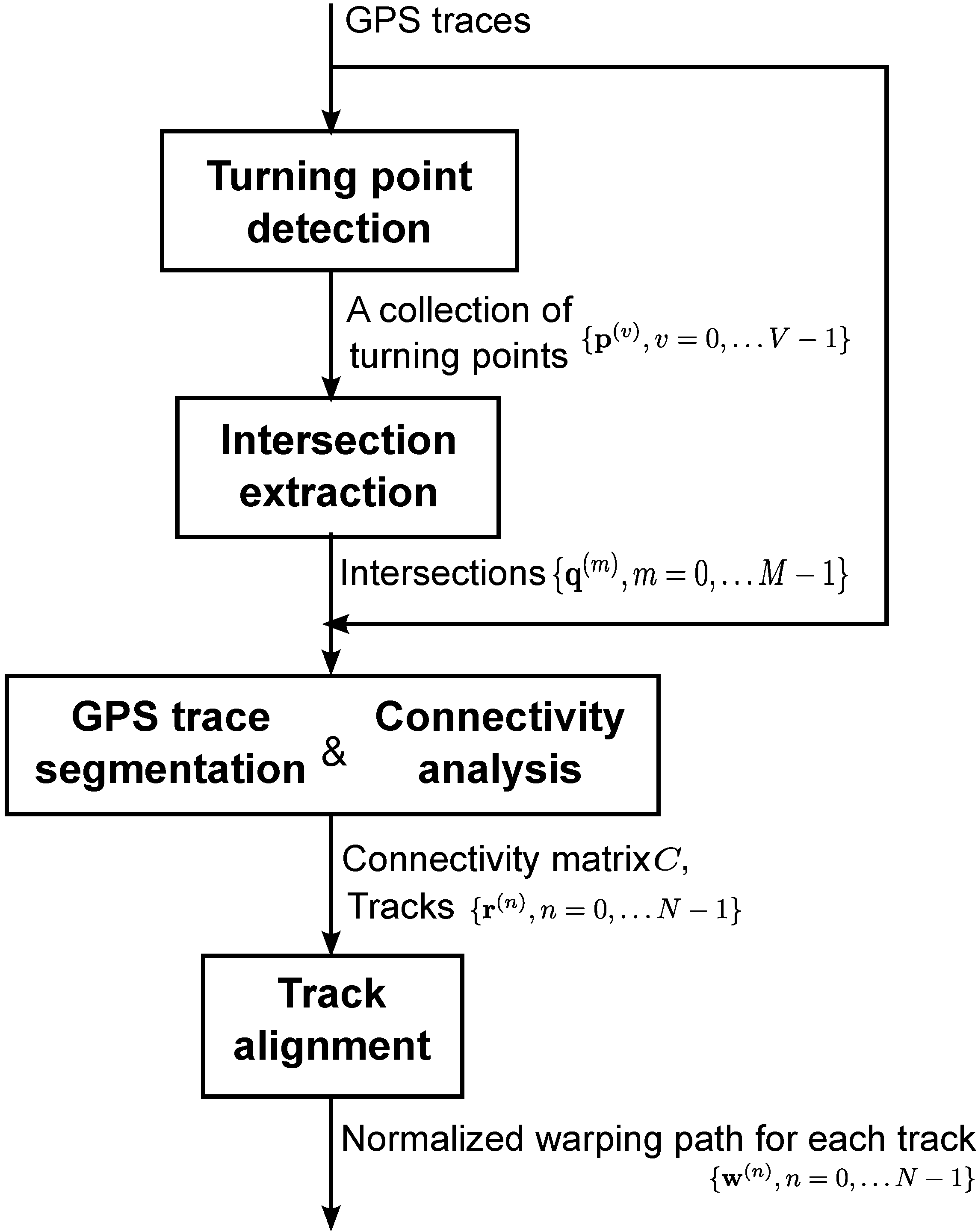
3. Road Network Inference

The main elements of a more general transportation network include intersections, roads, railways, highways, motor vehicular lanes, bicycles and pedestrians lanes. However, we will only explore a subset of these elements in the form of a road network, which is a system that represents the interconnecting roads located in a given area. In order to clarify the scope of our work in this paper, we present the three elements that define a road network below.

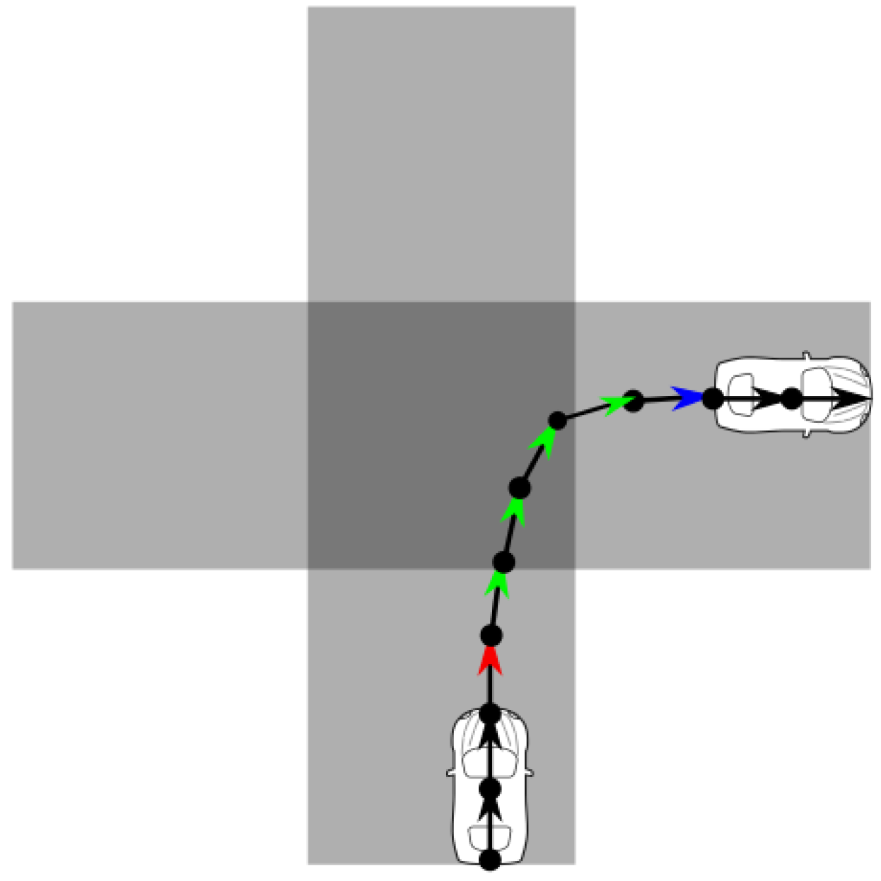
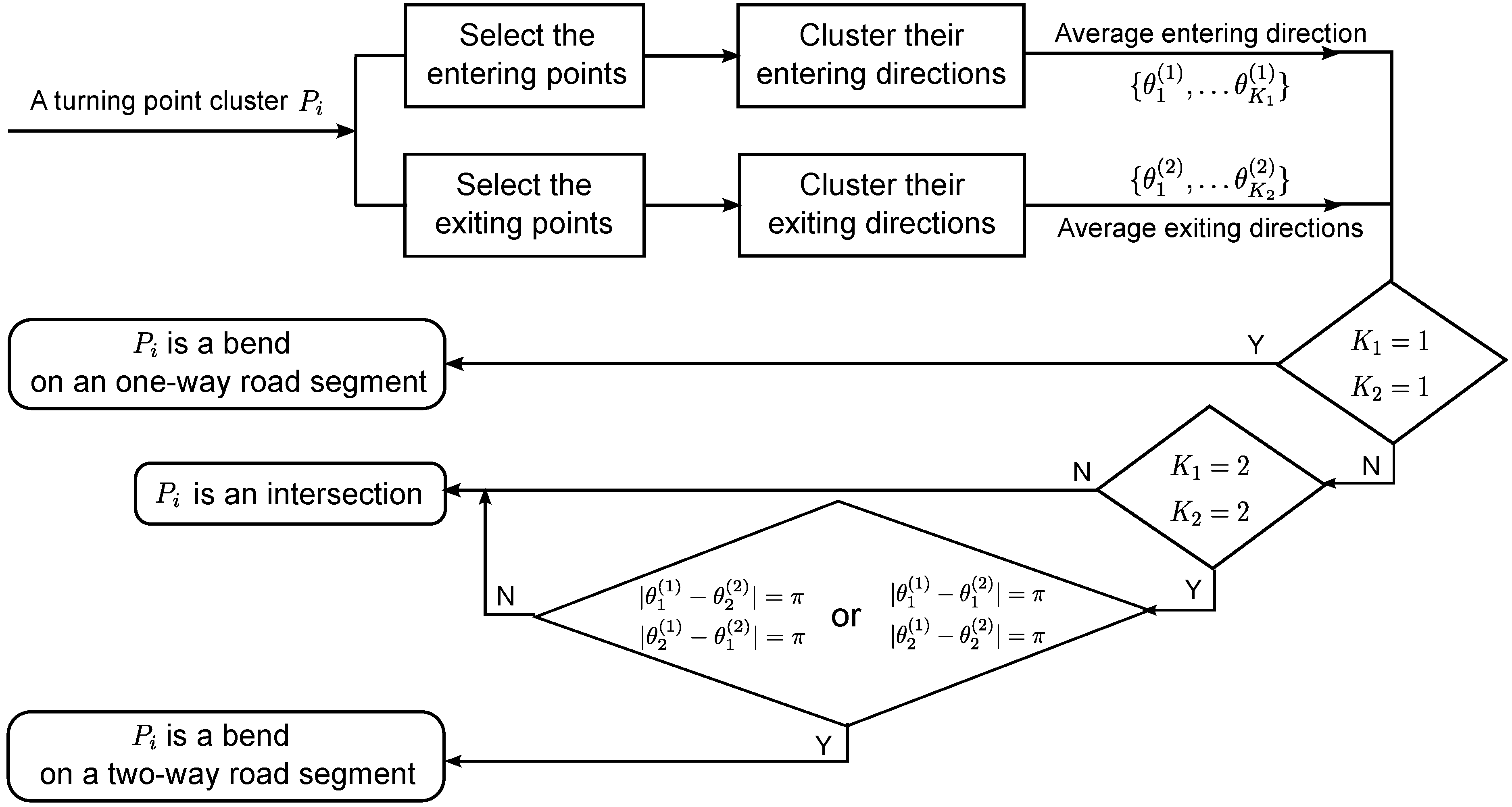
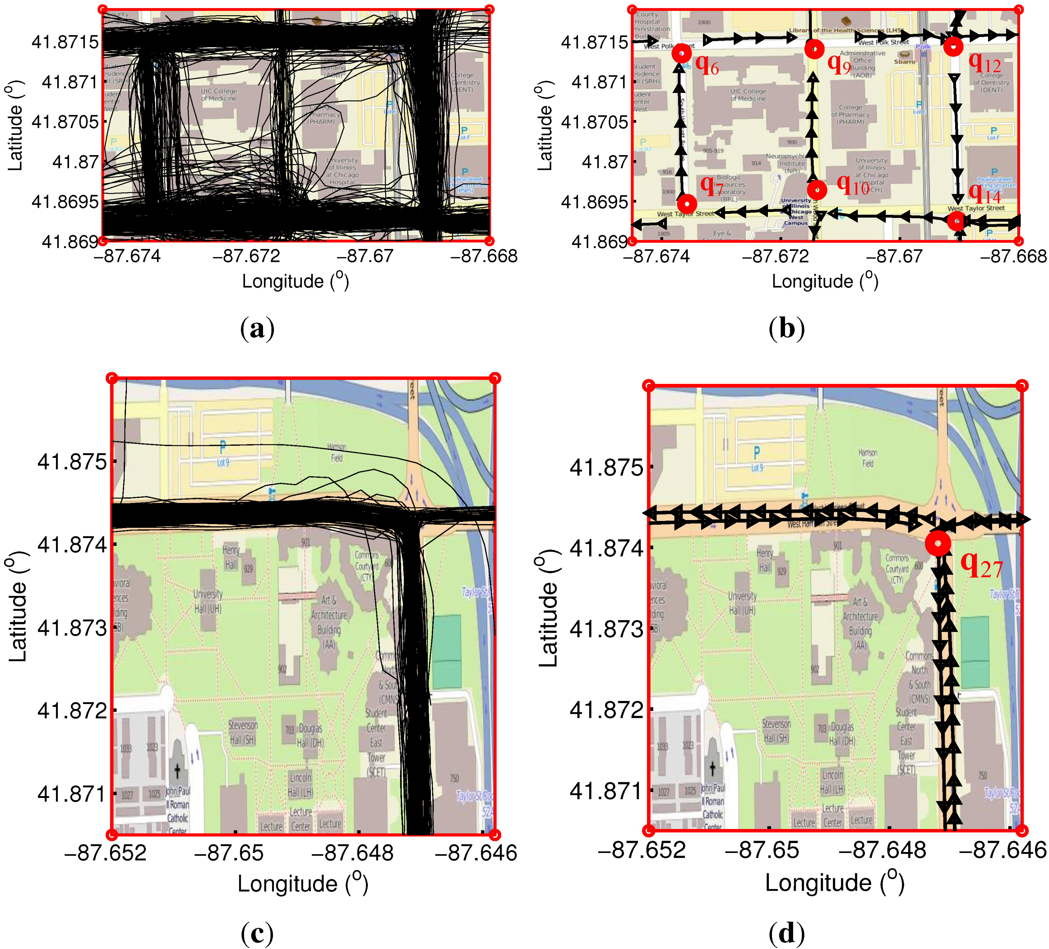
• Intersections: Road intersections are represented by their geographic position $\mathbf{\text{q}}={(x,y)}^T$, where x and y are coordinates in latitude and longitude. An intersection can be defined as a location where the users can change directions in multiple ways, regardless of the number of road segments meeting at a particular intersection. Intersections are unique from the bends in roads, which only allow the users to make a single change in direction.
• Connectivity graph: Road connectivity graphs encode if a pair of intersections are directly connected by a road segment containing no other intersections. These graphs are represented by a binary $M\times M$ connectivity matrix C, with M the number of intersections. By definition, $C_{i,j}=1$ if intersections i and j are directly connected by a single road segment. In our paper, C is asymmetric, i.e., $C_{i,j}$ can differ from $C_{j,i}$ due to one-way traffic. Moreover, we assume that the main diagonal elements of C are zero, i.e., an intersection is not connected to itself.
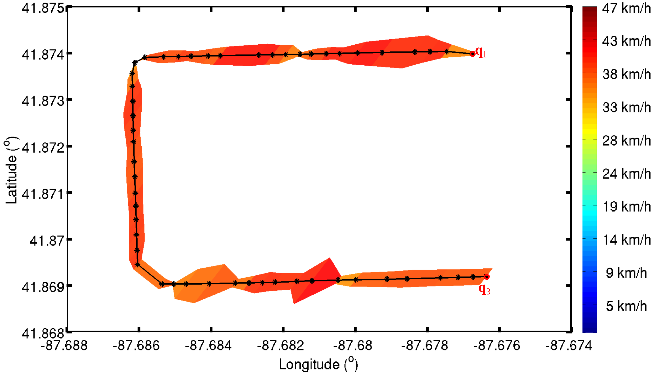
• Road segments: The directed road segments R connect pairs of intersections. The geometry of each road segment is represented using a sequence of geographical locations. In this paper, the average speed and speed variance along each road segment will be analyzed using the GPS traces. However, the type of the road and the number of lanes on the road will not be analyzed.

Figure 1 presents an overview of our method. First, we group turning points of individual traces into intersections using our clustering method, without using prior knowledge of the number of intersections.

Second, we segment all GPS traces based on the detected intersections. GPS device users often follow different routes to the same destination, creating different GPS traces with variable speeds and locations. However, all traces will share common segments corresponding to individual road segments.

Lastly, we align all of the tracks for each road segment, point by point, using DTW with a “stretch and then compress” strategy. The aligned tracks are averaged to form a representation for each road segment. The track alignment outperforms the existing methods in generating cleaner road networks without spurious edges. It also allows for the statistical analysis of the variance of traffic speeds represented by the tracks that compose each road segment.

3.1. Turning Point Detection

The intuition behind our turning point detection is that while some road users may travel straight through intersections, at least some of them will turn onto other roads at intersections. This turning behavior is not unique to intersections, as road users may also appear to make turns at bends in roads, which we do not consider intersections. Therefore, when we detect spatial locations where many tracks show turning points, we also perform an additional analysis to distinguish bends in roads from true cross roads, which is described in Section 3.2.

Figure 1. Overview of the proposed method.

Figure 1. Overview of the proposed method.

When the road users make turns at the intersections, the change in their moving direction over a fixed amount of time is different depending on their speed. Thus, it is difficult to choose a single threshold to detect the direction change to detect turns. To make the approach robust against speed differences, we calculate the change in the moving direction over a fixed distance. If the fixed distance is too small, the direction change at the intersections cannot be distinguished from the fluctuations in the moving direction. Based on our experience, the direction change over at least 2 m at the intersection can be adequately distinguished from the fluctuations. However, depending on the sampling rate of the GPS units and the speed of the road users, it is possible that the distance between two adjacent GPS points is larger than 2 m.

Therefore, the moving direction of the user at $(x_a,y_a)$ is computed as follows:

Given a point on a GPS trace, $(x_a,y_a)$, we select a second point, $(x_b,y_b)$, that is 2 m ahead on the same trace; if such a point does not exist, we select the next adjacent point. The moving direction of the user at $(x_a,y_a)$ is computed as:

$${\theta }_a=\left\{\begin{array}{cc}\text{arctan}\frac{y_b-y_a}{x_b-x_a}\hfill & x_b>x_a\hfill \\ \text{arctan}\frac{y_b-y_a}{x_b-x_a}+\pi \hfill & y_b\ge y_a,x_b<x_a\hfill \\ \text{arctan}\frac{y_b-y_a}{x_b-x_a}-\pi \hfill & y_b<y_a,x_b<x_a\hfill \\ -\frac{\pi }{2}\hfill & y_b>y_a,x_b=x_a\hfill \\ +\frac{\pi }{2}\hfill & y_b<y_a,x_b=x_a\hfill \end{array}\right.$$

(1)

where ${\theta }_a\in [-\pi ,\pi ]$ ($-\pi$ is west, radians counter-clockwise).

The moving direction of the user, ${\theta }_b$, at the point $(x_b,y_b)$ is calculated similarly using the the next point on the GPS trace that is a fixed distance away. If the direction change $\text{Δ}{\theta }_b={\theta }_b-{\theta }_a$ between the points $(x_a,y_a)$ and $(x_b,y_b)$ exceeds a predefined threshold, then it is considered as a turning point.

Since intersections are typically much larger than our two-meter turn detection distance threshold, many GPS points with direction changes can be detected inside of the same intersection. We consider all of the neighboring data points with direction changes detected from GPS traces as turning points. We keep track of the first and last point in a sequence of moving direction changes, which can represent the user entering and exiting the intersection respectively, which will be later used to distinguish bends in roads from true intersections. An example of a turn is shown in Figure 2, as the vehicle makes a right turn at the intersection. The moving directions of the turning points are shown with colored arrows, where red indicates the first turning point, blue indicates the last turning point and green for other turning points. The moving direction of other points without a direction change is shown as a black arrow.

Figure 2. An example of a turn. A part of a GPS trace around one intersection is represented by a black line with circles indicating the position of data recordings and arrows indicating the moving direction at each point.

Figure 2. An example of a turn. A part of a GPS trace around one intersection is represented by a black line with circles indicating the position of data recordings and arrows indicating the moving direction at each point.

The output of this step is a collection of turning points $\{{\mathbf{\text{p}}}^{\left(v\right)},v=0,\dots V-1\}$, which are detected by checking the change of moving direction at each point along all GPS traces, along with binary indicators of whether the user enters the intersection $\{e_1^v,v=0,\dots V-1\}$ or exits the intersection $\{e_2^{\left(v\right)},v=0,\dots V-1\}$ at a particular turning point, where $e_1^{\left(v\right)}\in [0,1]$ and $e_2^{\left(v\right)}\in [0,1]$. $e_1^{\left(v\right)}=1$ indicates that the user enters an intersection at the turning point v, and zero indicates not entering. We describe how these turning points will be clustered into intersections in the next section.

3.2. Intersection Extraction

In our work, we propose a clustering technique to group the collection of turning points P into intersections based on Euclidean distance. As shown in Algorithm 1, an initial cluster is grown from a seed point by iteratively adding points to the cluster if their average distance to the current points in the cluster is small enough. This procedure is then repeated on the points that have not yet been clustered. The output of this step is a set of clusters $P_i=\{{\mathbf{\text{p}}}_i^{\left(n\right)}$, $n=0\dots |P_i|-1\}$, with $|P_i|$ as the number of turning points per cluster. As a post-processing step, we also discard clusters that contain too few turning points; these may be caused by GPS noise or by an insufficient sampling of an intersection.

Algorithm 1 Cluster turning points.

Input: $\{{\mathbf{\text{p}}}^{\left(v\right)}$, $v=0\dots V-1\}$

Output: $\{P_i:|P_i|>T_{\text{min}}$$i=0\dots I-1\}$

1: Initialization $P_{un}\leftarrow \{{\mathbf{\text{p}}}^{\left(v\right)}$, $v=0\dots V-1\}$ $i\leftarrow 0$

2: for each $\mathbf{\text{p}}\in P_{un}$ do

3:      $P_{out}=\varnothing$, $P_i=\left\{\mathbf{\text{p}}\right\}$,

4:     for each ${\mathbf{\text{p}}}^{\prime }\ne \mathbf{\text{p}}\in P_{un}$ do

5:         if $\frac{1}{|P_i|}{\displaystyle \sum _{{\mathbf{\text{p}}}^{″}\in P_i}}d\left({\mathbf{\text{p}}}^{\prime },{\mathbf{\text{p}}}^{″}\right)\le d_{thre}$ then $d_{thre}$ is the predefined threshold for the average Euclidean distance.

6:             $P_i\leftarrow P_i\cup \left\{{\mathbf{\text{p}}}^{\prime }\right\}$

7:         end if

8:     end for

9:     $P_{un}=P_{un}\backslash P_i$

10: end for

To remove the misdetected road bends from the clusters, where road users may also change their moving direction, we need check for the type of turns for each cluster using the entering (with $e_1^{\left(v\right)}=1$) and exiting turning points (with $e_2^{\left(v\right)}=1$) as described in the previous step. As shown in Figure 3, we select the entering and exiting turning points and cluster their direction separately for each cluster of turning points. If the entering and exiting directions stay the same (for a one-way road segment) or are opposite (for a two-way road segment), this cluster will be removed, because the turning points in this cluster lie in a bend rather than an intersection.

Finally, the spatial locations ${\mathbf{\text{q}}}_m$ of the clusters are obtained by averaging the turning points in each cluster. The result is the set of intersections $Q=\{{\mathbf{\text{q}}}_m,m=0,\dots ,M-1\}$.

3.3. Connectivity Analysis and GPS Trace Segmentation

The connectivity of intersections is analyzed by determining if there are GPS traces that travel directly from one intersection to another. We first determine if a given GPS trace contains any intersections by computing the distance of each point in the trace with the location to our detected intersections. If the distance between a point in a trace and a intersection is within a predetermined threshold, we conclude that the GPS trace travels through an intersection. Ideally, two intersections are directly connected if there is a trace that travels directly through both intersections without encountering a third. However, GPS errors can contribute to false positive intersection connections if an intersection is not detected along a trace. For example, assume that a user travels through three intersections on one trace, but only the first and the last one are detected by our distance thresholding; the second one is missed because of GPS noise. This would lead to a false positive connectivity between the first and the third intersections.

Figure 3. Bend detection. Bends are detected by checking the entering and exiting directions.

Figure 3. Bend detection. Bends are detected by checking the entering and exiting directions.

In this paper, the number of traces traveling between two adjacent intersections are used to decide whether they are directly connected. After the connectivity is determined, we partition all GPS traces into track segments between each pair of directly-connected intersections. The output of this step is the connectivity matrix C and the track segments associated with each road segment between intersections. We will use the following notations. For one road segment R, there are N tracks $\{{\mathbf{\text{r}}}^{\left(n\right)},n=0,\dots ,N-1\}$, with track n consisting of $L_n$ points ${\mathbf{\text{r}}}^{\left(n\right)}=({\mathbf{\text{r}}}^{\left(n\right)}\left(0\right),\dots ,{\mathbf{\text{r}}}^{\left(n\right)}(L_n-1))$. Specifically, ${\mathbf{\text{r}}}^{\left(n\right)}\left(i\right)=(x^{\left(n\right)}\left(i\right),y^{\left(n\right)}\left(i\right))$ is composed of the the latitude and longitude of point i in track n.

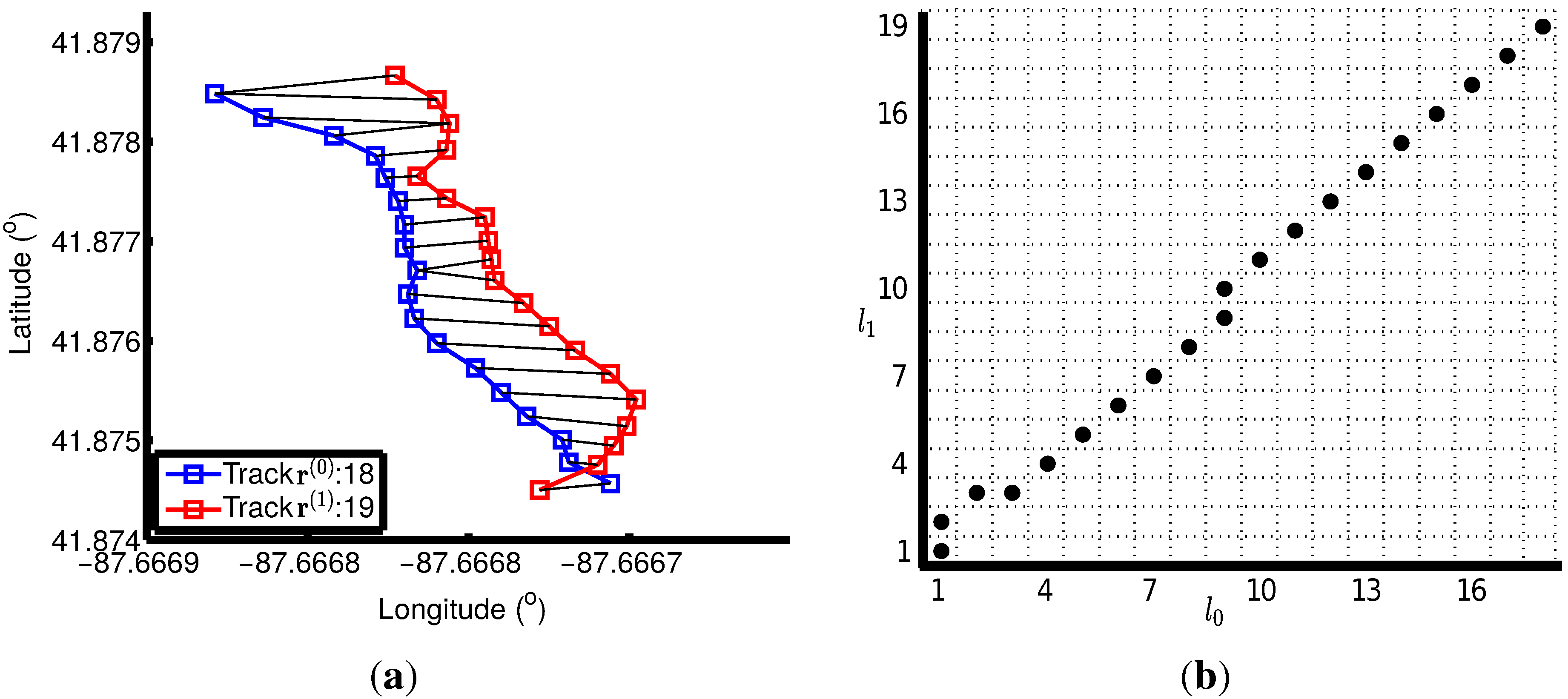
3.4. Track Alignment

For the same road segment, the GPS tracks begin and end at the same two intersections. Although the geographical distance that each track covers is similar to the length of the road segment, the spatial GPS point density of tracks varies because vehicles can move at different speeds. Less GPS points are recorded if the user travels through the road with higher speed and vice versa. The main task of this section is to find point correspondences between all of the tracks and to average them to form a single representation of the road segment. However, reliably detecting corresponding points is difficult because of the varying speeds on each track. Some naive methods could produce temporally-inconsistent matches. In this paper, we apply dynamic time warping (DTW) to solve this problem. We begin by explaining the principle of DTW for use with two-track alignment and then generalize the approach using our “stretch and then compress” strategy for multiple track alignment. The average track will be calculated using the alignments of the tracks.

3.4.1. Two-Track Alignment Using DTW

DTW is a time series alignment algorithm developed originally for speech recognition [25]. It attempts to find a time alignment between two signals that maximizes a similarity measure between samples of the two signals by warping their time axis.

Given two tracks of points $({\mathbf{\text{r}}}^{\left(0\right)}\left(0\right),\dots ,{\mathbf{\text{r}}}^{\left(0\right)}(L_0-1)$ and $({\mathbf{\text{r}}}^{\left(1\right)}\left(0\right),\dots ,{\mathbf{\text{r}}}^{\left(1\right)}(L_1-1)$ and a distance measure between pairs of points, the problem of finding the best alignment can be described as finding an association $(l_0\left(0\right),\dots ,l_0(K_0-1))$ and $(l_1\left(0\right),\dots ,l_1(K_0-1))$ that minimizes the aggregate distance.

$$D_{\Gamma }\left({\mathbf{\text{r}}}^{\left(0\right)},{\mathbf{\text{r}}}^{\left(1\right)}\right)\stackrel{▵}{=}\underset{(l_0,l_1)\in \Gamma }{min}\sum _{k_0=0}^{K_0-1}{∥{\mathbf{\text{r}}}^{\left(0\right)}\left(l_0\left(k_0\right)\right)-{\mathbf{\text{r}}}^{\left(1\right)}\left(l_1\left(k_0\right)\right)∥}^2$$

(2)

where $l_0\left(k_0\right)$ and $l_0\left(k_0\right)$ associate corresponding time instances $l_0$ of the first track and $l_1$ of the second track. Not all such associations are allowed. Specifically, we consider only warp paths, which belong to a subset Γ of all possible associations and which satisfy the following restrictions:

• Boundary conditions: The warp path must start at the beginning of each time series and end at the end of each time series: $l_0\left(0\right)=0$, $l_0(K_0-1)=L_0-1$, $l_1\left(0\right)=0$ and $l_1(K_0-1)=L_0-1$.
• Monotonicity: The warp path must be monotonically nondecreasing along both time axes: $l_0\left(k_0\right)\le l_0(k_0+1)$ and $l_1\left(k_0\right)\le l_1(k_0+1)$.
• Continuity: Any two adjacent steps of the warp paths follow the $(l_0\left(k_0\right)-l_0(k_0-1),l_1\left(k_0\right)-l_1(k_0-1))\in \{(0,1),(1,0),(1,1)\}$. With this constraint, the warp path for each track moves at most one point at a time.

After computing the functions $l_0\left(k_0\right)$ and $l_1\left(k_0\right)$, the tracks ${\mathbf{\text{r}}}^{\left(0\right)}$ and ${\mathbf{\text{r}}}^{\left(1\right)}$ are now aligned in the sense that they reach close spatial positions at the same index k, resulting in new warped tracks with $K_0$ points ${\mathbf{\text{r}}}_1^{\left(0\right)}=({\mathbf{\text{r}}}_1^{\left(0\right)}\left(0\right),\dots ,{\mathbf{\text{r}}}_1^{\left(0\right)}(K_0-1))$ and ${\mathbf{\text{r}}}_1^{\left(1\right)}=({\mathbf{\text{r}}}_1^{\left(1\right)}\left(0\right),\dots ,{\mathbf{\text{r}}}_1^{\left(1\right)}(K_0-1))$, where ${\mathbf{\text{r}}}_1^{\left(0\right)}\left(k_0\right)={\mathbf{\text{r}}}^{\left(0\right)}\left(l_0\left(k_0\right)\right)$ and ${\mathbf{\text{r}}}_1^{\left(1\right)}\left(k_0\right)={\mathbf{\text{r}}}^{\left(1\right)}\left(l_1\left(k_0\right)\right)$. To obtain an optimal alignment, it is probable that these warped tracks have duplicated points.

To align two tracks using DTW, we first compute a distance matrix $D_{L_0\times L_1}^{\left(1\right)}$ for each pair of GPS points in both tracks, where the element $d^{\left(1\right)}(l_0,l_1)$ at the $l_0$-th row and $l_1$-th column of $D^{\left(1\right)}{L}_0\times L_1$ represents the distance between the $\left(l_0\right)$-th point in Track ${\mathbf{\text{r}}}^{\left(0\right)}$ and the $\left(l_1\right)$-th point in Track ${\mathbf{\text{r}}}^{\left(1\right)}$. We then calculate the accumulated distance matrix $D_{L_0\times L_1}^{\left(2\right)}$ from the distance matrix $D_{L_0\times L_1}^{\left(1\right)}$, where the element $d^{\left(2\right)}(l_0,l_1)$ at $(l_0,l_1)$ in $D_{L_0\times L_1}^{\left(2\right)}$ is computed by adding the $d^{\left(1\right)}(l_0,l_1)$ together with the minimum value of $\left\{d^{\left(2\right)}(l_0-1,l_1),d^{\left(2\right)}(l_0,l_1-1),d^{\left(2\right)}(l_0-1,l_1-1)\right\}$.

The warp paths are then searched from the accumulated matrix $D^{\left(2\right)}$ in descending order, starting at $d^{\left(2\right)}(L_0,L_1)$ and ending at $d^{\left(2\right)}(1,1)$ under the boundary conditions. The previous step $({\mathbf{\text{w}}}^{\left(0\right)}(k_0-1),{\mathbf{\text{w}}}^{\left(1\right)}(k_0-1)$) in the paths is chosen from the position of the element with the smallest value from the adjacent elements with one-step decreasing indexes $\left\{d^{\left(2\right)}(l_0-1,l_1),d^{\left(2\right)}(l_0,l_1-1),d^{\left(2\right)}(l_0-1,l_1-1)\right\}$. This ensures that the search procedure satisfies the continuity and monotonic conditions.

An example of aligning two tracks is shown in Figure 4. There are 18 points in Track ${\mathbf{\text{r}}}^{\left(0\right)}$, which is represented by a blue line with squares indicating the positions of data points. Track ${\mathbf{\text{r}}}^{\left(1\right)}$ is depicted as a red line with squares indicating the position of its 19 points. The matching pairs of these two tracks are shown by linking the points using a black line. In Figure 4b, the horizontal axis of this grid map is the time axis of Track ${\mathbf{\text{r}}}^{\left(0\right)}$, and the vertical one is for Track ${\mathbf{\text{r}}}^{\left(1\right)}$. The best alignment of Track ${\mathbf{\text{r}}}^{\left(0\right)}$ and ${\mathbf{\text{r}}}^{\left(1\right)}$ can be described as finding a path through the grid from the left-bottom grid $(1,1)$ to the right-top grid $(18,19)$ with the smallest overall distance between all pairs of points. The best warp path in this case is shown in solid round circles. According to the optimal warp path, both of the tracks are extended to 20 elements.

Figure 4. Example of two-track alignment. (a) The elements in two tracks are paired using DTW with the distance between these elements as features. (b) the warp path with the horizontal and the vertical axis indicates the time index of Track ${\mathbf{\text{r}}}^{\left(0\right)}$ and Track ${\mathbf{\text{r}}}^{\left(1\right)}$ separately.

Figure 4. Example of two-track alignment. (a) The elements in two tracks are paired using DTW with the distance between these elements as features. (b) the warp path with the horizontal and the vertical axis indicates the time index of Track ${\mathbf{\text{r}}}^{\left(0\right)}$ and Track ${\mathbf{\text{r}}}^{\left(1\right)}$ separately.

Because of GPS errors or data loss, some of the tracks do not fit along the physical “road,” although they share the same starting and ending points. The spatial distance of one track ${\mathbf{\text{r}}}^{\left(n\right)}$ to all of other tracks belonging to the same road segment is calculated as ${\sum }_{m\ne n,m=0}^{m=N_i-1}S({\mathbf{\text{r}}}^{\left(n\right)},{\mathbf{\text{r}}}^{\left(m\right)})$, while $S({\mathbf{\text{r}}}^{\left(n\right)},{\mathbf{\text{r}}}^{\left(m\right)})$ is the mean spatial distance between two tracks.

$$S({\mathbf{\text{r}}}^{\left(n\right)},{\mathbf{\text{r}}}^{\left(m\right)})\stackrel{▵}{=}\frac{1}{K}{D}_{\Gamma }\left({\mathbf{\text{r}}}^{\left(n\right)},{\mathbf{\text{r}}}^{\left(m\right)}\right)$$

(3)

where K is the length of their warp paths.

If the average spatial distance of one track to other tracks exceeds a predefined value, it will not be used to do the track alignment for this road. This will remove the tracks with high GPS errors and large data loss.

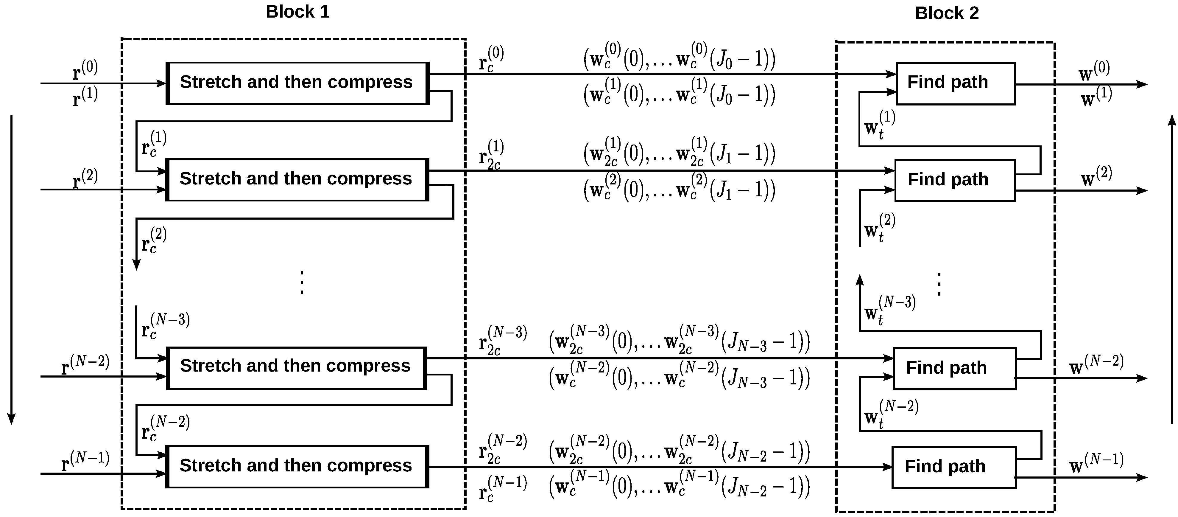
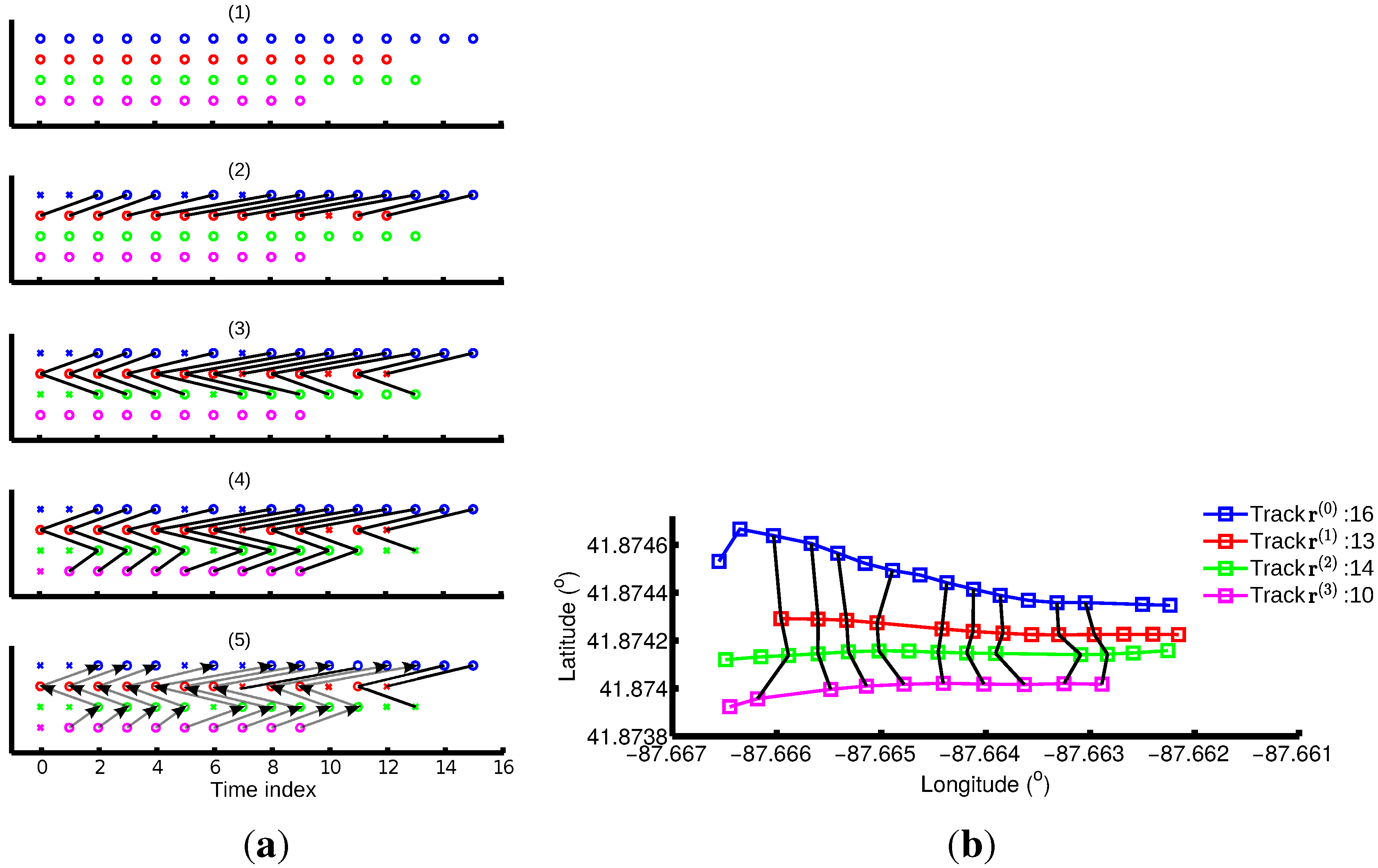
3.4.2. “Stretch and then Compress” Strategy

The DTW procedure only allows the aligning of two tracks. For different pairs of tracks, their warp paths and the length of the warped tracks can be different. Therefore, it is difficult to find a normalized path to align all possible pairs of tracks together. We now propose a “stretch and then compress” strategy to enable multiple track alignment of all tracks. This strategy is composed of two different operations, a (1) stretch operation followed by a (2) compress operation, as described below.

(1) Stretch: Track ${\mathbf{\text{r}}}^{\left(0\right)}$ with $L_0$ points and Track ${\mathbf{\text{r}}}^{\left(1\right)}$ with $L_1$ points are warped to Track $({\mathbf{\text{r}}}^{\left(0\right)}\left(l_0\left(0\right)\right),\dots ,{\mathbf{\text{r}}}^{\left(0\right)}\left(l_0(K_0-1)\right))$ and Track $({\mathbf{\text{r}}}^{\left(1\right)}\left(l_1\left(0\right)\right),\dots ,{\mathbf{\text{r}}}^{\left(1\right)}\left(l_1(K_0-1)\right))$ separately using DTW to stretch both tracks to contain $K_0$ points. Some points of one track with similar locations are matched to the same point in the other track; therefore, the points in the warped tracks are repetitions of the points in the original tracks. The warped track is not shorter than both original tracks, i.e., $K_0⩾L_{0}and{K}_0⩾L_1$, which is called “stretch”.

(2) Compress: Some points of one track are matched to the same point in the other track, leading to the many-to-one correspondence between the data points in the stretched tracks. We compress the stretched tracks by shrinking their data points, which are warped from the same data point in the original track. We keep only the point with the shortest distance to the corresponding point in the other stretched track. In this way, the stretched tracks $({\mathbf{\text{r}}}^{\left(0\right)}\left(l_0\left(0\right)\right),\dots ,{\mathbf{\text{r}}}^{\left(0\right)}\left(l_0(K_0-1)\right))$ and $({\mathbf{\text{r}}}^{\left(1\right)}\left(l_1\left(0\right)\right),\dots ,{\mathbf{\text{r}}}^{\left(1\right)}\left(l_1(K_0-1)\right))$ are compressed to Track ${\mathbf{\text{r}}}_c^{\left(0\right)}$ and ${\mathbf{\text{r}}}_c^{\left(1\right)}$ with $J_0$ points, creating compressing paths ${\mathbf{\text{w}}}_c^{\left(0\right)}$ and ${\mathbf{\text{w}}}_c^{\left(1\right)}$, where ${\mathbf{\text{r}}}_c^{\left(0\right)}\left(j_0\right)={\mathbf{\text{r}}}^{\left(0\right)}\left(l_0\left(k_0\left(j_0\right)\right)\right)$, ${\mathbf{\text{r}}}_c^{\left(1\right)}\left(j_0\right)={\mathbf{\text{r}}}^{\left(1\right)}\left(l_1\left(k_0\left(j_0\right)\right)\right)$, ${\mathbf{\text{w}}}_c^{\left(0\right)}\left(j_0\right)=l_0\left(k_0\left(j_0\right)\right)$ and ${\mathbf{\text{w}}}_c^{\left(1\right)}\left(j_0\right)=l_1\left(k_0\left(j_0\right)\right)$. $l_0\left(k_0\left(j_0\right)\right)$ is the location index of the $j_0$-th point of the compressed track ${\mathbf{\text{r}}}_c^{\left(0\right)}$ in the original track ${\mathbf{\text{r}}}^{\left(0\right)}$ and is the location index of the $j_0$-th point of the compressed track ${\mathbf{\text{r}}}_c^{\left(1\right)}$ in the original track ${\mathbf{\text{r}}}^{\left(1\right)}$. The data point of one compressed track only corresponds to one data point of another compressed track at the same time index, which is called a one-to-one correspondence. By compressing the tracks, they are shorter than the original tracks, i.e., $J_0⩽L_{0}and{J}_0⩽L_1$.

3.4.3. Multiple Track Alignment

We align multiple tracks by first applying the “stretch and then compress” strategy to process all of the tracks one by one from the first to the last track sequentially.

Block 1 in Figure 5 illustrates the procedure presented below:

(A) Track ${\mathbf{\text{r}}}^{\left(0\right)}$ with $L_0$ points and Track ${\mathbf{\text{r}}}^{\left(1\right)}$ with $L_1$ points are inputs to the “stretch and then compress” module, in order to get the once-compressed tracks, ${\mathbf{\text{r}}}_c^{\left(0\right)}$ and ${\mathbf{\text{r}}}_c^{\left(1\right)}$. The compressing paths ${\mathbf{\text{w}}}_c^{\left(0\right)}$ and ${\mathbf{\text{w}}}_c^{\left(1\right)}$ describe the location indexes of Track ${\mathbf{\text{r}}}_c^{\left(0\right)}$ and Track ${\mathbf{\text{r}}}_c^{\left(1\right)}$ in the original tracks, ${\mathbf{\text{r}}}^{\left(0\right)}$ and ${\mathbf{\text{r}}}^{\left(1\right)}$, separately, where c means once compressed here.

(B) Once-compressed Track ${\mathbf{\text{r}}}_c^{\left(1\right)}$ and Track ${\mathbf{\text{r}}}^{\left(2\right)}$ are inputs to the “stretch and then compress” module, resulting in twice-compressed Track ${\mathbf{\text{r}}}_{2c}^{\left(1\right)}$ and once-compressed Track ${\mathbf{\text{r}}}_c^{\left(2\right)}$, where $2c$ means twice compressed here. The compressing paths ${\mathbf{\text{w}}}_{2c}^{\left(1\right)}$ save the time indexes of the twice-compressed track ${\mathbf{\text{r}}}_{2c}^{\left(1\right)}$ in the once-compressed track ${\mathbf{\text{r}}}_c^{\left(1\right)}$ and ${\mathbf{\text{w}}}_c^{\left(2\right)}$ for time indexes of the once-compressed track ${\mathbf{\text{r}}}_c^{\left(2\right)}$ in the original track ${\mathbf{\text{r}}}^{\left(2\right)}$.

(C) Once-compressed Track ${\mathbf{\text{r}}}_c^{\left(n\right)}$ and a new track, ${\mathbf{\text{r}}}^{(n+1)}$, are input to the “stretch and then compress” module, until the last track ${\mathbf{\text{r}}}^{(N-1)}$ is processed.

The outputs of Block 1 are the once-compressed tracks for the first and the last track ${\mathbf{\text{r}}}_c^{\left(0\right)}$ and ${\mathbf{\text{r}}}_c^{(N-1)}$, the twice-compressed tracks for the other tracks $\{{\mathbf{\text{r}}}_{2c}^{\left(n\right)},n=1,\dots ,N-2\}$, the compressing paths $\{{\mathbf{\text{w}}}_c^{\left(n\right)},n=0,\dots ,N-1\}$, which keep the time indexes of the once-compressed tracks in the original tracks, and compressing paths $\{{\mathbf{\text{w}}}_{2c}^{\left(n\right)},n=1,\dots ,N-2\}$ for the locations indexes of the twice-compressed tracks in the once-compressed tracks.

Figure 5. Multiple-track alignment. In Block 1, the tracks are aligned one by one in random order using a “stretch and then compress”, producing intermediate paths; Block 2 depicts how to find the normalized paths, which are used to align all of the tracks with one-to-one correspondence among the points using intermediate paths produced in Block 1.

Figure 5. Multiple-track alignment. In Block 1, the tracks are aligned one by one in random order using a “stretch and then compress”, producing intermediate paths; Block 2 depicts how to find the normalized paths, which are used to align all of the tracks with one-to-one correspondence among the points using intermediate paths produced in Block 1.

Compression is necessary in Block 1, because each point in a compressed track has a unique corresponding point in the other compressed tracks. With the one-to-one correspondences, the points in other tracks corresponding to the points of ${\mathbf{\text{r}}}_{2c}^{\left(n\right)}$ can be easily located. Without the compression step, the tracks will be stretched longer and longer with many-to-one correspondence as new tracks are warped using DTW, leading to increasing computation cost.

Block 2 depicts how to find the normalized paths $\{{\mathbf{\text{w}}}^{\left(n\right)},n=0,\dots ,N-1\}$ that align all of the tracks with one-to-one correspondence among the points using intermediate paths $\{{\mathbf{\text{w}}}_t^{\left(n\right)},n=N-2,\dots ,1\}$, resulting in the normalized tracks $\{{\mathbf{g}}^{\left(n\right)},n=0,\dots N-1\}$ with the same length. The normalized path ${\mathbf{\text{w}}}^{\left(n\right)}$ keeps the location information of the points of the normalized track ${\mathbf{g}}^{\left(n\right)}$ in the original track ${\mathbf{\text{r}}}^{\left(n\right)}$.

Among the output tracks from Block 1, the last once-compressed track ${\mathbf{\text{r}}}_c^{(N-1)}$ with $J_{N-2}$ points is the shortest track, since $J_n$ is always shorter than $J_{n-1}$. In our method, ${\mathbf{\text{r}}}_c^{(N-1)}$ is taken as the normalized track ${\mathbf{g}}^{(N-1)}$ for Track ${\mathbf{\text{r}}}^{(N-1)}$. For the other tracks, the data points that correspond to ${\mathbf{g}}^{(N-1)}$ are first selected from the twice-compressed tracks. The time indexes of data points of ${\mathbf{g}}^{\left(n\right)}$ in ${\mathbf{\text{r}}}_c^{\left(n\right)}$ are indexed using a intermediate path ${\mathbf{\text{w}}}_t^{\left(n\right)}$, where t refers to a temporary intermediate path. The time indexes of the data points of ${\mathbf{g}}^{\left(n\right)}$ in the original input track ${\mathbf{\text{r}}}^{\left(n\right)}$ can be found using the intermediate path ${\mathbf{\text{w}}}_t^{\left(n\right)}$ and the warp path ${\mathbf{\text{w}}}_c^{\left(n\right)}$:

$${\mathbf{\text{w}}}_t^{\left(n\right)}=\left\{\begin{array}{cc}{\mathbf{\text{w}}}_{2c}^{(N-2)}\hfill & n=N-2\hfill \\ {\mathbf{\text{w}}}_{2c}^{\left(n\right)}\left({\mathbf{\text{w}}}_t^{(n+1)}\right)\hfill & n=N-3,\dots ,1\hfill \end{array}\right.$$

(4)

$${\mathbf{\text{w}}}^{\left(n\right)}=\left\{\begin{array}{cc}{\mathbf{\text{w}}}_c^{(N-1)}\hfill & n=N-1\hfill \\ {\mathbf{\text{w}}}_c^{\left(n\right)}\left({\mathbf{\text{w}}}_t^{\left(n\right)}\right)\hfill & n=N-2,\dots ,0\hfill \end{array}\right.$$

(5)

The normalized track ${\mathbf{g}}^{\left(n\right)}$ is obtained by selecting $K=J_{N-2}$ points from ${\mathbf{\text{r}}}^{\left(n\right)}$ according to its normalized warp path ${\mathbf{\text{w}}}^{\left(n\right)}$, i.e., ${\mathbf{g}}^{\left(n\right)}={\mathbf{\text{r}}}^{\left(n\right)}\left({\mathbf{\text{w}}}^{\left(n\right)}\right)$.

Figure 6. Example of four track alignment. (a) shows the data points of the tracks along time. In Sub-figure 2, Tracks ${\mathbf{\text{r}}}^{\left(0\right)}$ and ${\mathbf{\text{r}}}^{\left(1\right)}$ are stretched and compressed, resulting in ${\mathbf{\text{r}}}_c^{\left(0\right)}$ and ${\mathbf{\text{r}}}_c^{\left(1\right)}$, with black lines indicating their association. A once-compressed track and a new track are input to the “stretch and then compress” module, so as to find the one-to-one correspondence among the tracks in Sub-figures 3 and 4. Sub-figure 5 depicts how to find the normalized path by the connecting lines. (b) shows how the data points of normalized tracks are selected from the original tracks along the normalized path and connected using black lines.

Figure 6. Example of four track alignment. (a) shows the data points of the tracks along time. In Sub-figure 2, Tracks ${\mathbf{\text{r}}}^{\left(0\right)}$ and ${\mathbf{\text{r}}}^{\left(1\right)}$ are stretched and compressed, resulting in ${\mathbf{\text{r}}}_c^{\left(0\right)}$ and ${\mathbf{\text{r}}}_c^{\left(1\right)}$, with black lines indicating their association. A once-compressed track and a new track are input to the “stretch and then compress” module, so as to find the one-to-one correspondence among the tracks in Sub-figures 3 and 4. Sub-figure 5 depicts how to find the normalized path by the connecting lines. (b) shows how the data points of normalized tracks are selected from the original tracks along the normalized path and connected using black lines.

An example of four track alignment is shown in Figure 6. The points of each track along the time axis are shown in circles with different colors. If a point is removed from the track by the “compress” procedure, it is indicated using a cross. In the first sub-figure of Figure 6a, all of the data points are shown as circles, because the track alignment has not started. In its second sub-figure, ${\mathbf{\text{r}}}^{\left(0\right)}$ and ${\mathbf{\text{r}}}^{\left(1\right)}$ are inputs to the “ stretch and then compress” module, resulting in ${\mathbf{\text{r}}}_c^{\left(0\right)}$ and ${\mathbf{\text{r}}}_c^{\left(1\right)}$, which are shown in circles and connected with black lines. Five points in ${\mathbf{\text{r}}}^{\left(0\right)}$ and one in ${\mathbf{\text{r}}}^{\left(1\right)}$ are removed. The next sub-figure shows the results of Tracks ${\mathbf{\text{r}}}_c^{\left(1\right)}$ and ${\mathbf{\text{r}}}^{\left(2\right)}$ alignment as connected lines from ${\mathbf{\text{r}}}_{2c}^{\left(1\right)}$ to ${\mathbf{\text{r}}}_c^{\left(2\right)}$. In the fourth sub-figure, ${\mathbf{\text{r}}}_{2c}^{\left(2\right)}$ and ${\mathbf{\text{r}}}_c^{\left(3\right)}$ are stretched and compressed from ${\mathbf{\text{r}}}_c^{\left(2\right)}$ and ${\mathbf{\text{r}}}^{\left(3\right)}$ separately. The data points of other tracks that correspond to ${\mathbf{\text{r}}}_c^{\left(3\right)}$ can be located from bottom to top by following the connecting lines, i.e., the compressing paths. Figure 6b shows the physical locations of points for each track. There are 16, 13, 14 and 10 points respectively in these four tracks. After the alignment, nine data points in each track are kept, which are associated with each other.

3.5. Statistical Analysis

In this paper, we use the average of all of the tracks as the geometric representation of a road segment. Because the tracks have different lengths, averaging them directly at time indexes will lead to inaccurate results. With the normalized tracks $\{{\mathbf{g}}^{\left(n\right)},n=0,\dots ,N-1\}$ with the same length K, which are warped according to the normalized warp paths $\{{\mathbf{\text{w}}}^{\left(n\right)},n=0,\dots ,N-1\}$, the average track $\mathbf{g}=\left(\mathbf{g}\right(0),\dots ,\mathbf{g}(K-1\left)\right)$ can be extracted from the normalized tracks along the warp paths.

$$\mathbf{g}\left(k\right)=\frac{1}{N}\sum _{n=0}^{N-1}{\mathbf{g}}^{\left(n\right)}\left(k\right)$$

(6)

Given the speed at each point of the normalized track $({\mathbf{s}}^{\left(n\right)}\left(0\right),\dots ,{\mathbf{s}}^{\left(n\right)}(K-1)$, where $n=0,\dots ,N-1\}$, the average speed, $\mu \left(k\right)$, and speed variance, $\delta \left(k\right)$, along the average track are calculated as below:

$$\mu \left(k\right)=\frac{1}{N}\sum _{n=0}^{N-1}{\mathbf{s}}^{\left(n\right)}\left(k\right)$$

(7)

$$\delta \left(k\right)=\frac{1}{N}\sum _{n=0}^{N-1}{({\mathbf{s}}^{\left(n\right)}\left(k\right)-\mu \left(k\right))}^2$$

(8)

where $k=0,\dots ,K-1$.

4. Evaluation of Algorithm Performance

In order to evaluate the performance of our proposed algorithm, we need to calculate the accuracy of the generated road network, which consists of intersections, their connectivity and the road segment representations. The generated road network has to be accurate, both topologically and geometrically, with respect to a ground truth map. The topological accuracy of the road network describes how many intersections are extracted in the road network and their connectivity. For example, whether each pair of intersections are connected to each other and, if so, whether the connection is one-directional or two-directional. The geometric accuracy refers to how accurate the geographic locations contained in the road network are compared to the ground truth map. Both the geographic locations of the intersections and the sequences of data points representing the roads segments need to be evaluated.

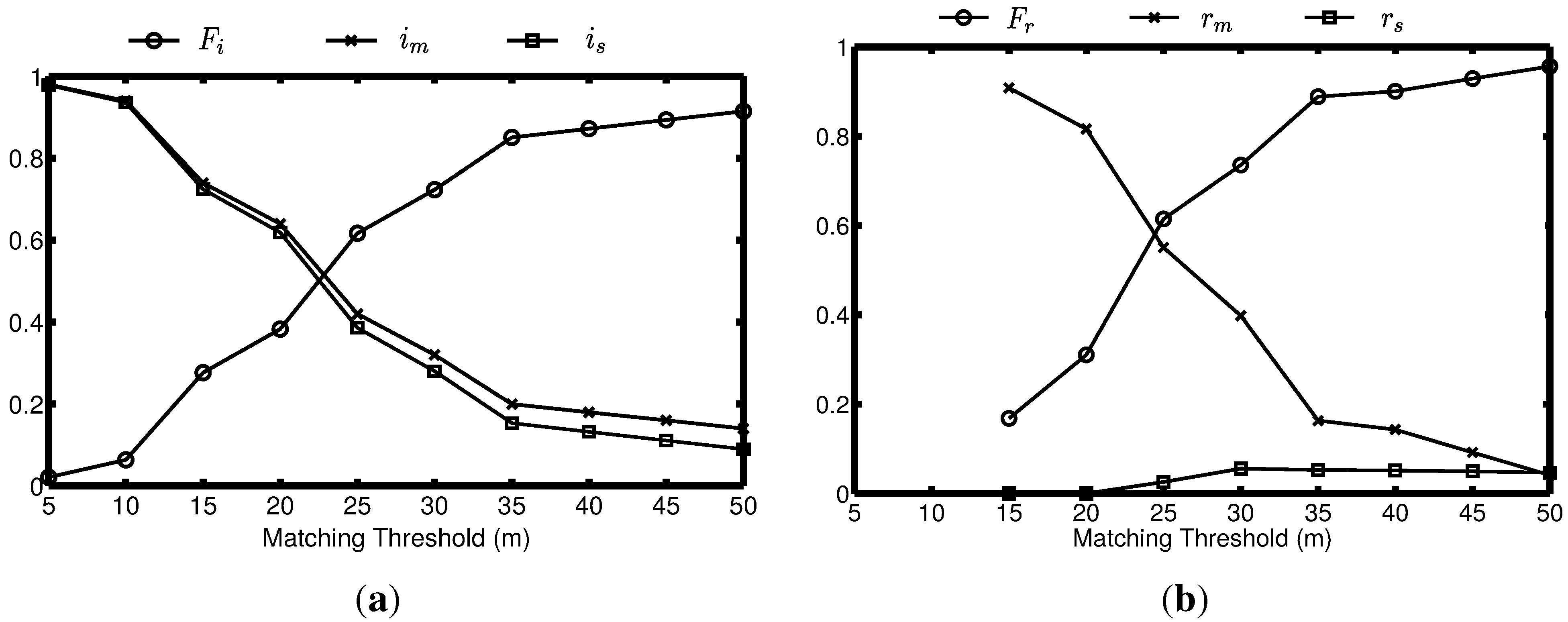
4.1. Topological Accuracy Calculation

Our intersections are extracted from GPS traces. Due to the limited accuracy and outliers in the GPS traces, we may both detect “spurious” intersections that do not exist on the ground truth map, and we may also fail to detect some real intersections (i.e., which exist in the ground truth map). The accuracy of the intersections depends on three primary aspects: the number of “matched” intersections that are detected successfully, the number of “spurious” intersections and the number of “missing” intersections.

In this paper, we use two parameters to quantify the accuracy of the intersections: $i_s$, the proportion of “spurious” intersections, and $i_m$, the proportion of “missing” intersections [16]; both are defined below.

$$\begin{array}{c}{i}_s=\frac{I_s}{I_s+I_c}\\ \\ i_m=\frac{I_m}{I_m+I_c}\end{array}$$

(9)

where $I_s$ is the number of spurious intersections, $I_c$ the number of correctly-matched intersections and $I_m$ the number of non-matched, i.e., missing intersections.

The well-known F-score, based on a combination of precision and recall, is used as an overall quality score:

$$\begin{array}{c}{F}_i=2\frac{(1-i_s)(1-i_m)}{(1-i_s)+(1-i_m)}\end{array}$$

(10)

Higher values of the $F_i$-score indicate that the intersection detection is more accurate [21].

Similar to the intersection quality indicators, we also define quality indicators for the connectivity between intersections: $r_s$ is the proportion of spuriously-detected road segments that do not exist on the ground truth map, $r_m$ the proportion of “missing” road segments that exist in the ground truth map, but fail to be detected, and $F_r$ the corresponding F score.

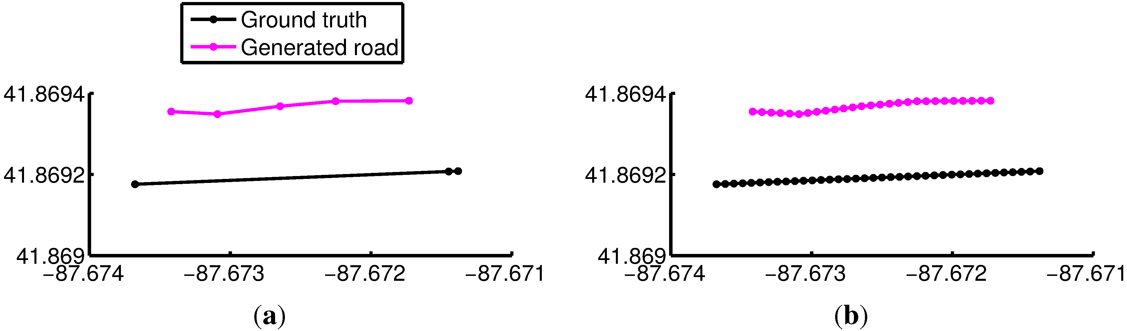
4.2. Geographical Accuracy Evaluation

Measuring the accuracy of the generated roads compared to the ground truth map is related to the topic of map matching. As the first step, this requires matching road segments from the experimental results with those in the ground truth map. A variety of algorithms can be applied to solve this problem [26], for example Kalman filtering, fuzzy logic and many others. In our case, the road segment can be identified easily by finding the corresponding intersections through checking the distance between the data points on the ground truth map and the intersections, since in this dataset, at most one directed road segment exists between each pair of intersections.

To judge the difference between an inferred road segment (as produced by the algorithm in Section 3.4.3 and the corresponding road segment in the ground truth map, we could naively compute a measure based on the distance between points in both road segments. However, this poses some complications, as the inferred road segments in our paper are represented as a sequence of data points (the average of points of time-aligned tracks). The available ground truth road segments are also represented as a time series of data points. However, both the total number of points per road segment and its distribution over time can vary considerably between the inferred and ground truth data and from one road segment to another. Therefore, any quality measures based on distances between points in the ground truth and inferred road segments are affected by this variability.

A partial solution would be to apply DTW to align the two point series and to warp them to new series of the same length, then compute the quality measure on those warped track segments. However, this does not fully solve the problem, as the warped series can only contain repeated points, but can never “fill in” missing data. Therefore, large time gaps in the ground truth or inferred data could lead to large spatial distances between ground truth and inferred data, even if the track segments are otherwise very similar. For instance, the first and second points of the generated road in Figure 7a are matched to the first point on the ground truth using DTW, because no closer points are found on the ground truth. The distance between these paired points are actually larger than the real distance between the generated road segment and its ground truth [27].

Figure 7. Example of a single road. (a) shows a generated road segment and its ground truth as an example. (b) shows them after interpolation, so as to reduce the error of their distance caused by the uneven distribution of the data points on the road.

Figure 7. Example of a single road. (a) shows a generated road segment and its ground truth as an example. (b) shows them after interpolation, so as to reduce the error of their distance caused by the uneven distribution of the data points on the road.

In this paper, we approach this problem by interpolating the data points of both the inferred and ground truth road segments. The interpolation limits the spatial distance between successive points on the same road segment to a one meter, as shown in Figure 7b, and then, we calculate the average distance between the paired interpolated data points through DTW as the distance between the generated road segment and its ground truth. Through interpolation, the data points are more dense and distributed more evenly, reducing the error of the distance measurement.

5. Experiments

A data set of 889 GPS traces over 118 h from the University of Illinois campus shuttles is used to test the proposed algorithm. This dataset can be accessed publicly on their BITSlaboratory website [28]. The GPS data are gathered by campus shuttle drivers who carry an iPhone running the BITS Laboratory’s tracking application. Although their iPhone application sends its GPS location to their server every second, the server sometimes fails to receive the GPS data, leading to a varying sampling interval of 1 s to 29 s (average: 3.61 s; standard deviation: 3.67 s). Although their GPS recordings are from the same device, our method does not require the same sampling rate. The participating shuttles travel through both areas with low-rise buildings and other areas with significant GPS error because of tall buildings. The raw GPS traces are depicted in black lines in Figure 8.

To measure the accuracy of the road network generated from the shuttle traces, we choose OpenStreetMap as the ground truth map. Although the positional error of GPS traces on OpenStreetMap is approximately 10 to 20 m, it is still popularly used as the ground truth for research in road network generation, because of its open source access and large coverage. Because the shuttles did not explore all streets in the OpenStreetMap [29], the generated road network only covers where the shuttles traveled. The ground truth map is manually reduced to the streets that were actually traversed by the shuttles. Figure 9 shows the ground truth map with red circles for intersections and black lines with black solid circles for road segments.

Figure 8. Intersection extraction. Intersections in red circles are detected from the turning points in green dots, where the shuttles change their moving directions.

Figure 8. Intersection extraction. Intersections in red circles are detected from the turning points in green dots, where the shuttles change their moving directions.

Figure 9. Ground truth map. The directed ground truth map is manually made through reducing the OpenStreetMap of this area to the streets traversed by the shuttles.

Figure 9. Ground truth map. The directed ground truth map is manually made through reducing the OpenStreetMap of this area to the streets traversed by the shuttles.

5.1. Results Using Our Method

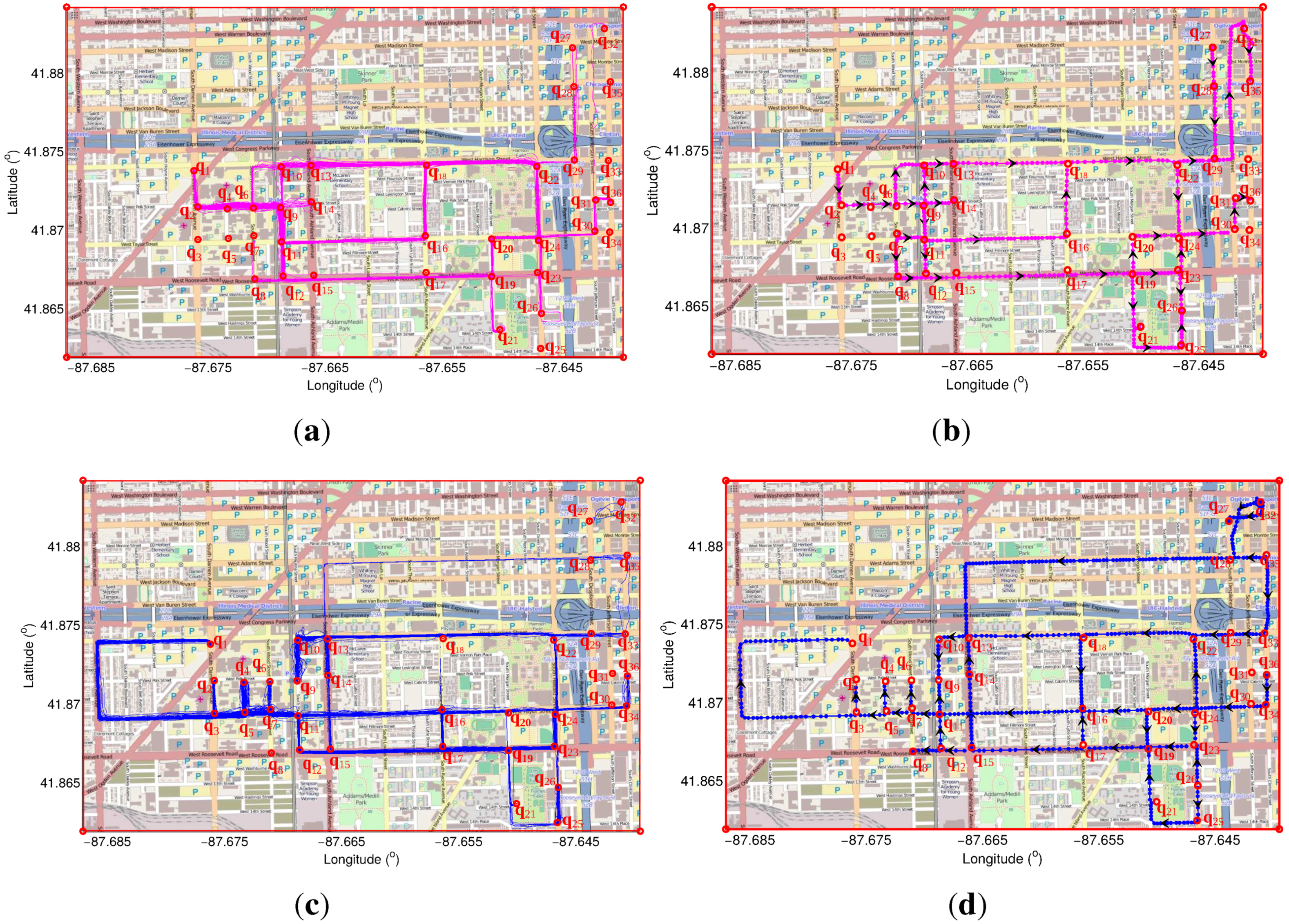
5.1.1. Inferred Turning Points and Intersections

In Figure 8, the turning points extracted from all 889 GPS traces are depicted as red dots. The locations where many turning points gather and are recognized as intersections are shown in green dots in Figure 8. Sometimes, isolated turning points are detected because of GPS errors or insufficient coverage from the shuttle. These isolated turning points are not considered as intersections in our algorithm. Figure 8 shows an intersection that apparently exists between ${\mathbf{\text{q}}}_{14}$ and ${\mathbf{\text{q}}}_{15}$. However, no intersection is detected there using our method, because there are only a few isolated turning points.

At this location, the shuttle always goes straight without changing its direction, possibly because of the presence of a bridge. Moreover, there are two intersections on the ground truth map around the location of extracted intersection ${\mathbf{\text{q}}}_{26}$ using our method. We found that the turning points are clustered in the same group ${\mathbf{\text{q}}}_{26}$, because they are too close to each other. The bends where the road users always turn in the same directions are not recognized as intersections. For instance, the two bends at the left edge of the map are removed from the intersections. In total, 36 intersections, which are shown as red circles in Figure 8, are detected from the turning points, while there are actually 33 intersections on the ground truth map, as shown in Figure 9. More intersection are detected using our method because of GPS noise.

On the ground truth map, each intersection is localized at the center of the junction between road segments. However, the intersections detected using our method sometimes deviate from the center, depending on the type of turns the shuttle makes at a particular junction. For instance, the intersection ${\mathbf{\text{q}}}_{22}$ connects four road segments, but the shuttle only visited three of them. Additionally, the shuttle only made one type of turn there: coming from ${\mathbf{\text{q}}}_{18}$, turning right at ${\mathbf{\text{q}}}_{22}$ to ${\mathbf{\text{q}}}_{24}$. Therefore, the detected intersection ${\mathbf{\text{q}}}_{22}$ drifted toward the direction of ${\mathbf{\text{q}}}_{24}$. The average distance between the detected intersections and their ground truth is $22.69$ m.

Figure 10a depicts the tracks as magenta lines, for the roads that start from lower index intersections and end with intersections with a higher index. Figure 10b shows the generated roads from these tracks with arrows indicating the directions of the roads; while the tracks shown in blue lines in Figure 10c are for the roads from higher index intersections to lower index intersections and Figure 10d for the generated directed roads from these tracks. In total, 38 roads are extracted in Figure 10b and 39 in Figure 10d, which means that 77 pairs of intersections are connected to each other directly. From Figure 10, we also know that some of the roads are one way, for instance the road segment between the first and third intersection. The shuttles always travel from ${\mathbf{\text{q}}}_1$ to ${\mathbf{\text{q}}}_3$ and never take the opposite direction. In another case, the shuttles travel between the intersection ${\mathbf{\text{q}}}_{22}$ and ${\mathbf{\text{q}}}_{29}$ in both direction according to their GPS traces. However, there is no road segment existing between them on the ground truth map, as shown in Figure 9. This could be caused by temporary road construction. The Chicago dataset was recorded in April 2011, but OpenStreetMap was accessed in August 2014. By checking this road segment under Google street view on dates closest to the access dates, the road between intersection ${\mathbf{\text{q}}}_{22}$ and ${\mathbf{\text{q}}}_{29}$ was accessible in May 2011, but was blocked because of road construction in October 2014.

Figure 10. Directed roads. (a) shows part of the tracks, which are averaged to produce the directed roads in (b) ; (c) shows the other part of the tracks, which are averaged to produce the directed roads in (d).

Figure 10. Directed roads. (a) shows part of the tracks, which are averaged to produce the directed roads in (b) ; (c) shows the other part of the tracks, which are averaged to produce the directed roads in (d).

5.1.2. Inferred Roads

Figure 10 shows the directed roads in each direction separately.

For each road segment, the average speed and the speed variation along the data points of the average track calculated in Section 3.5 are shown in Figure 11. The color of the points represents the strengths of the speed, and the width of the band around the average track indicates the variation of the speed.

5.1.3. Results Evaluation

Figure 12 shows the topological accuracy of the generated road network, with Figure 12a showing the accuracy of the intersections and Figure 12b showing the connectivity accuracy. The matching threshold is defined as the allowable distance between the intersections and their positions on the ground truth map. We can see that with the lowest 5-m matching threshold shown in Figure 12a, no matched intersections are detected. In this case, all of the intersections on the generated road network are classified as spurious intersections and all of the intersections on the ground truth map as missing intersections. As the matching threshold gets bigger, more intersections are detected and matched to the ground truth, resulting in lower $i_s$ and $i_m$ and higher $F_i$. Figure 12b shows the accuracy of the connectivity between the detected intersections. In our generated road network, no spurious edges are present, although sometimes, intersections are incorrectly connected. Such errors affect the $F_r$ number. With 5- and 10-meter matching thresholds, there are only a few intersections matched on the generated road network and the ground truth map. However, these intersections are not connected to each other, so no quantitative results are shown at these two thresholds in Figure 12b.

Figure 11. Statistic analysis. The speed and the speed variation along the road segment from Intersection ${\mathbf{\text{q}}}_3$ to ${\mathbf{\text{q}}}_1$ are depicted.

Figure 11. Statistic analysis. The speed and the speed variation along the road segment from Intersection ${\mathbf{\text{q}}}_3$ to ${\mathbf{\text{q}}}_1$ are depicted.

Figure 12. Topological accuracy evaluation. (a) shows the accuracy of the generated intersections; (b) shows the accuracy of the connectivity between the intersections. With different matching distances between the generated intersections and their ground truth. The bigger the F-score is, the more accurate its is.

Figure 12. Topological accuracy evaluation. (a) shows the accuracy of the generated intersections; (b) shows the accuracy of the connectivity between the intersections. With different matching distances between the generated intersections and their ground truth. The bigger the F-score is, the more accurate its is.

With 50 m as the matching threshold for the intersections, there are 77 directed roads detected in our paper. The average distance between all of the generated roads and their ground truth is used to describe the geographical accuracy of the generated road network, which is calculated as $7.35$ m.

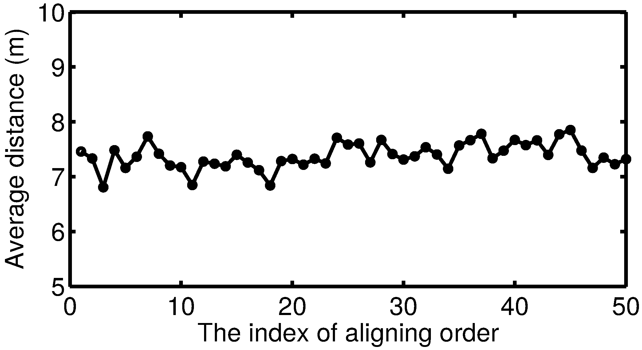
5.1.4. Discussion of How the Aligning Order Affects the Results

Since we stretch and compress the tracks one by one, the tracks that are inputs to Block 1 earlier should have more influence on the results. Especially if GPS data points of one track are removed during the compress phase, the data points in other tracks that are matched to these removed points later will also be removed using our algorithm, leading to unbalanced influence. However, the tracks that are used to extract the road segment are quite similar to each other. Additionally outlier tracks with a lower similarity score are removed and not used to do the track alignment. In this case, in which order to align the tracks will not have a large effect on the results.

The results shown in Figure 10 are extracted from the tracks using an order based on their similarity score to other tracks, which is calculated as the sum of their similarity score to every other track. To evaluate the influence quantitatively, we also averaged the tracks by aligning them in 50 other random orders. The average distance between the generated road segment and its ground truth with 50 different orders is calculated and shown in Figure 13. The horizontal and vertical axis indicate the index of aligning order and the distance, respectively. No matter which order is selected to align the tracks, the distance from the generated road segment to the ground truth is always around $7.38$ m with maximum value $7.85$ m and minimum value $6.81$ m, which means the aligning order has no significant influence on averaging the tracks.

Figure 13. Influence of the aligning order. No matter in which order the tracks are aligned, the average distance between all of the generated roads and their ground truth is around $7.37$ m stably, which means the aligning order does not affect the track alignment significantly.

Figure 13. Influence of the aligning order. No matter in which order the tracks are aligned, the average distance between all of the generated roads and their ground truth is around $7.37$ m stably, which means the aligning order does not affect the track alignment significantly.

5.2. Comparison with Other Methods

Our results are compared to the existing methods as follows: the curve fitting method proposed by Schroedl [2], the KDE-based method by Davies [3] and also the trace-merging method proposed by Cao [4]. Since qualitative and quantitative evaluations of these three existing algorithms have been done in Biagioni and Eriksson in [16] using the same Chicago campus shuttle dataset as us, we can compare the results of their algorithms directly with ours.

Figure 14 shows the results of the same two examples that Biagioni used in his paper [16], one example with high-error GPS traces, while the other one with low-error GPS traces. Both Schroedl and Cao produced spurious road edges using the high-error GPS traces in Figure 14a, while our algorithm, based on intersection detection, extracted the road topology successfully without adding any extraneous edges. Although Davies also produced clean roads, our method still outperforms his, because our generated roads are directed, while he only extracted undirected roads.

Figure 14a shows part of the tracks, which are averaged to produce the directed roads in Figure 14b; Figure 14c shows the other part of the tracks, which are averaged to produce the directed roads in Figure 14d.

Figure 14. Comparison with other methods. (a) shows the some high-error GPS traces, which are used to extract the directed roads in (b); the traces in (c) have relatively low error, resulting in the directed roads in (d) .

Figure 14. Comparison with other methods. (a) shows the some high-error GPS traces, which are used to extract the directed roads in (b); the traces in (c) have relatively low error, resulting in the directed roads in (d) .

Additionally, 83 percent of the roads are detected within 10 meters of their ground truths, which outperforms all of the methods mentioned above whose F-scores are less than $0.7$ with a 15-meter matching threshold, as shown in Figure 6 in [16].

6. Conclusions and Future Work

We have presented a novel approach to infer a road network by extracting intersections, inferring their topology and segmenting road segments between intersections using GPS traces. We also form geometric representations of each road segment by aligning and averaging the tracks for each road segment using a “stretch and then compress” strategy. The tracks are aligned, point by point, through our “stretch” operation in the time dimension using DTW, and the redundant points are removed using our “compress” operation, resulting in one-to-one correspondence among the points in all of the tracks. The track alignment is also beneficial for further statistical analysis of the tracks, such as speed analysis and traveling time dynamics at the specific locations.

Although our algorithm outperforms other existing methods, our “compress” strategy will produce less data points as the road representation if there are small GPS data losses on any track or some tracks’ sampling frequency is lower than others. This is since tracks with high GPS data loss or with extraordinarily low sampling frequency are clustered as outliers and will not be aligned together with other tracks. Therefore, in the future, we will focus on aligning tracks without the “compress” strategy and, therefore, keeping the many-to-one correspondence among the points in all of the tracks. Additionally, we will work on inferring the existence and coverage of intersections and road segments statistically using a probabilistic method, instead of the two-valued logic in our current method. We also intend to test our algorithm in areas with more complicated road features, such as overpasses, non-orthogonal road segments and roundabouts.

References

1. Biagioni, J.; Eriksson, J. Map inference in the face of noise and disparity. In Proceedings of the 20th International Conference on Advances in Geographic Information Systems, Redondo Beach, CA, USA, 7–9 November 2012; ACM: New York, NY, USA, 2012; pp. 79–88. [Google Scholar]
2. Schroedl, S.; Wagstaff, K.; Rogers, S.; Langley, P.; Wilson, C. Mining GPS traces for map refinement. Data Min. Knowl. Discov. 2004, 9, 59–87. [Google Scholar] [CrossRef]
3. Davics, J.; Beresford, A.R.; Hopper, A. Scalable, distributed, real-time map generation. IEEE Pervasive Comput. 2006, 5, 47–54. [Google Scholar]
4. Cao, L.; Krumm, J. From GPS traces to a routable road map. In Proceedings of the 17th ACM SIGSPATIAL International Conference on Advances in Geographic Information Systems, Seattle, WA, USA, 4–6 November 2009.
5. Shi, W.; Shen, S.; Liu, Y. Automatic generation of road network map from massive GPS, vehicle trajectories. In Proceedings of the IEEE 12th International Conference on Intelligent Transportation Systems, St. Louis, MO, USA, 4–7 October 2009.
6. Sato, J.; Takahashi, T.; Ide, I.; Murase, H. Change detection in streetscapes from GPS coordinated omni-directional image sequences. In Proceedings of the IEEE 18th International Conference on Pattern Recognition, Hong Kong, China, 20–24 August 2006.
7. Vlahogianni, E.I.; Karlaftis, M.G.; Golias, J.C. Optimized and meta-optimized neural networks for short-term traffic flow prediction: A genetic approach. Transp. Res. Part C Emerg. Technol. 2005, 13, 211–234. [Google Scholar] [CrossRef]
8. Syberfeldt, A.; Persson, L. Using Heuristic Search for Initiating the Genetic Population in Simulation-Based Optimization of Vehicle Routing Problems. In Proceedings of the Industrial Simulation Conference, EUROSIS-ETI, Loughborough, UK, 1–3 June 2009.
9. Schultes, D. Route Planning in Road Networks. Ph.D. Thesis, Karlsruhe Institute of Technology, Karlsruhe, Germany, 2008. [Google Scholar]
10. Niehoefer, B.; Burda, R.; Wietfeld, C.; Bauer, F.; Lueert, O. GPS community map generation for enhanced routing methods based on trace-collection by mobile phones. In Proceedings of the IEEE 1st International Conference on Advances in Satellite and Space Communications, Colmar, France, 20–25 July 2009.
11. Kukko, A.; Andrei, C.O.; Salminen, V.M.; Kaartinen, H.; Chen, Y.; Rönnholm, P.; Hyyppä, H.; Hyyppä, J.; Chen, R.; Haggrén, H.; et al. Road environment mapping system of the Finnish Geodetic InstituteâĂŤFGI Roamer. Int. Arch. Photogramm. Remote Sens. Spat. Inf. Sci. 2007, 36, 241–247. [Google Scholar]
12. Bellens, R.; Vlassenroot, S.; Gautama, S. Collection and analyses of crowd travel behaviour data by using smartphones. In Proceedings of the BIVEC-GIBET 5th Transport Research Day, Namur, Belgium, 25 May 2011.
13. Lee, D.; Hahn, M. Bicycle safety map system based on smartphone aided sensor network. Adv. Sci. Technol. Lett. 2013, 42, 38–43. [Google Scholar]
14. Haklay, M.; Weber, P. Openstreetmap: User-generated street maps. IEEE Pervasive Comput. 2008, 7, 12–18. [Google Scholar] [CrossRef]
15. Haklay, M. How good is volunteered geographical information? A comparative study of OpenStreetMap and Ordnance Survey datasets. Environ. Plan. B Plan. Des. 2010, 37, 682–703. [Google Scholar] [CrossRef]
16. Biagioni, J.; Eriksson, J. Inferring road maps from global positioning system traces. Transp. Res. Rec. J. Transp. Res. Board 2012, 2291, 61–71. [Google Scholar] [CrossRef]
17. Zheng, Y.; Li, Q.; Chen, Y.; Xie, X.; Ma, W.Y. Understanding mobility based on GPS data. In Proceedings of the 10th International Conference on Ubiquitous Computing, Seoul, Korea, 21–24 September 2008.
18. Edelkamp, S.; Schrödl, S. Route planning and map inference with global positioning traces. In Computer Science in Perspective; Springer: Berlin, Germany; Heidelberg, Germany, 2003; pp. 128–151. [Google Scholar]
19. You, Q.; Krumm, J. Transit tomography using probabilistic time geography: Planning routes without a road map. J. Locat. Based Serv. 2014, 8, 211–228. [Google Scholar] [CrossRef]
20. Xie, X.; Philips, W.; Veelaert, P.; Aghajan, H. Road network inference from GPS traces using DTW algorithm. In Proceedings of the IEEE 17th International Conference on Intelligent Transportation Systems (ITSC), Qingdao, China, 8–11 October 2014; pp. 906–911.
21. Liu, B. Web Data Mining; Springer: Berlin, Germany; Heidelberg, Germany, 2007. [Google Scholar]
22. Chen, C.; Cheng, Y. Roads digital map generation with multi-track gps data. In Proceedings of the IEEE InternationalWorkshop on Education Technology and Training, 2008. and 2008 International Workshop on Geoscience and Remote Sensing, Shanghai, China, 21–22 December 2008.
23. Morris, S.; Morris, A.; Barnard, K. Digital trail libraries. In Proceedings of the 4th ACM/IEEE-CS Joint Conference on Digital Libraries, Tucson, AZ, USA, 7–11 June 2004; ACM: New York, NY, USA, 2004. [Google Scholar]
24. Karagiorgou, S.; Pfoser, D. On vehicle tracking data-based road network generation. In Proceedings of the 20th International Conference on Advances in Geographic Information Systems, Redondo Beach, CA, USA, 7–9 November 2012.
25. Berndt, D.J.; Clifford, J. Using Dynamic Time Warping to Find Patterns in Time Series; KDD: Seattle, WA, USA, 1994. [Google Scholar]
26. Greenfeld, J.S. Matching GPS observations to locations on a digital map. In Proceedings of the Transportation Research Board 81st Annual Meeting, Washington, DC, USA, 13–17 January 2002.
27. Calcagno, P.; Chilès, J.P.; Courrioux, G.; Guillen, A. Geological modelling from field data and geological knowledge: Part I. Modelling method coupling 3D potential-field interpolation and geological rules. Phys. Earth Planet. Inter. 2008, 171, 147–157. [Google Scholar] [CrossRef]
28. BITS Networked Systems Laboratory. Available online: http://bits.cs.uic.edu/ (accessed on 24 August 2015).
29. OpenStreetMap. Available online: http://www.openstreetmap.org/ (accessed on 24 August 2015).