Finding Causes of Irregular Headways Integrating Data Mining and AHP

Abstract

Irregular headways could reduce the public transit service level heavily. Finding out the exact causes of irregular headways will greatly help to develop efficient strategies aiming to improve transit service quality. This paper utilizes bus GPS data of Harbin to evaluate the headway performance and proposes a statistical method to identify the abnormal headways. Association mining is used to dig deeper and recognize six causes of bus bunching. The AHP, embedded data analysis, is applied to determine the weight of each cause in the case of that these causes are combined with each other constantly. Results show that the front bus has a greater effect on bus bunching than the following bus, and the traffic condition is the most critical factor affecting bus headway.

1. Introduction

Headway is one of the important indicators to evaluate the level of transit service, which reflects the service intervals of transit and the rationality of the allocation of public transportation resources. The stability of headway is very important, especially for passengers. The time reliability is the first to be affected. Once the headway of two adjacent buses is too short, there will be a long interval for the third bus coming and the waiting time of passengers is increased, maybe doubled. Additionally, the long headway produces more demand and affects the travel time of the bus to some extent. Furthermore, the front bus of a bunch, or the third bus after a bunch, has to transport more passengers and it would be crowded on the bus. Thus, the travel comfort of passengers is influenced dramatically. Evaluating and studying headway of public transport has an important significance to improving transit service reliability and the quality of urban public transit service.

With the popularization and application of automatic vehicle locating (AVL), the public transit vehicles are monitored using GPS in most cities. In Harbin, for example, there is a large amount of GPS data every day, recording the real-time location, arriving/leaving information, and other driving information. A great deal of knowledge exists in the objective bus GPS data, which is extremely useful to evaluate and improve the service level of public transit within different densities or departure frequencies of the public transportation network. In part, these observations motivated our study. Therefore, this paper contributes to identify the abnormal headways using spatial-temporal bus GPS data and dig deeper to find the detailed causes by integrating data mining and analytic hierarchy process (AHP) methods.

The contributions of this research lie in two aspects: in theory, focusing on the bus GPS data, a method integrating data mining and AHP is proposed. This method not only reflects the objective fact hidden in the spatial-temporal data, but also is considered as a systemic analysis method and an effective decision-making method. The work offers a new way to systematically study spatial-temporal data mining and knowledge discovery. In practical terms, an effective method to identify and deeply analyze the irregular headway, which is an important indicator of transit service, is proposed. These findings would provide significant help to improving the urban public transport service.

The remainder of this paper is organized as follows. The next section reviews the research actuality of bus headway and transit spatial-temporal data analysis. The third section describes the bus route and the data studied. The headway performance is evaluated and abnormal headways are identified in the following section. In the fifth section, data mining and AHP are integrated to find the essential reasons for headway abnormity, and the final section concludes this paper.

2. Literature Review

At present, research on bus headway is mostly theoretical, seeking satisfying ways to improve the transit service. Thus, a variety of methods, such as holding [1,2,3,4,5], stop-skipping [6,7], and other hybrid control measures [8,9,10], are proposed to solve the bus bunching problem enabling buses to run following the pre-published schedule or maintaining the uniform headway. It is easy to find that the reason why these methods are difficult to be applied to practice is that some key factors change greatly in temporal and spatial scales, such as traffic condition and transit demand. Then, the spatial-temporal data of public transport is recognized as an effective foundation.

The existing transit spatial-temporal data mainly contains GPS data and integrated circuit (IC) card data. As soon as the data emerges, it is considered to be very precious and beneficial. There has been a surge of interest in transit data mining and analysis. This research mostly focuses on transit demand characteristics, transit service evaluation, and the running characteristics of buses. Bus IC data is often used in public transport origin-destination (OD) matrix estimation [11], user behavior mining [12], and other demand characteristics analysis [13]. The GPS data usually helps in evaluating the transit service performance, such as the service reliability [14,15], travel time reliability [16], evaluation index of transit quality identification [17], and performance measuring [18]. The running characteristics of bus analysis mainly concentrates on bus arrival time prediction [19,20]. As for the bus headway, the AVL data and IC data have been used to analyze the relationship between headway deviation and the number of on board passengers, as well as between running time variation and operator years of experience [21,22]. Significant relationships have been found statistically. There are also some explorations on the causes of abnormal headways. Originally, two causes, which are on-street effects and effects of the departure time at terminal, are analyzed using time-space trajectory graphs of several bus trips. Results showed that most of the headway problems originate as a result of irregular headways at the terminals [23,24]. Subsequently, empirical findings show that travel time between bus stops and dwell time at stops are the most two key causes of irregular headways [25] and several possible reasons are identified. These causes do not happen separately in most cases, and are combined with each other constantly. Thus, it is critical to find the exact causes in time and space of irregular headways and determine the weight of each cause to conduct the improvement measures. This is exactly one of the contributions of this paper.

3. Route Configuration and Data Description

3.1. Route Configuration

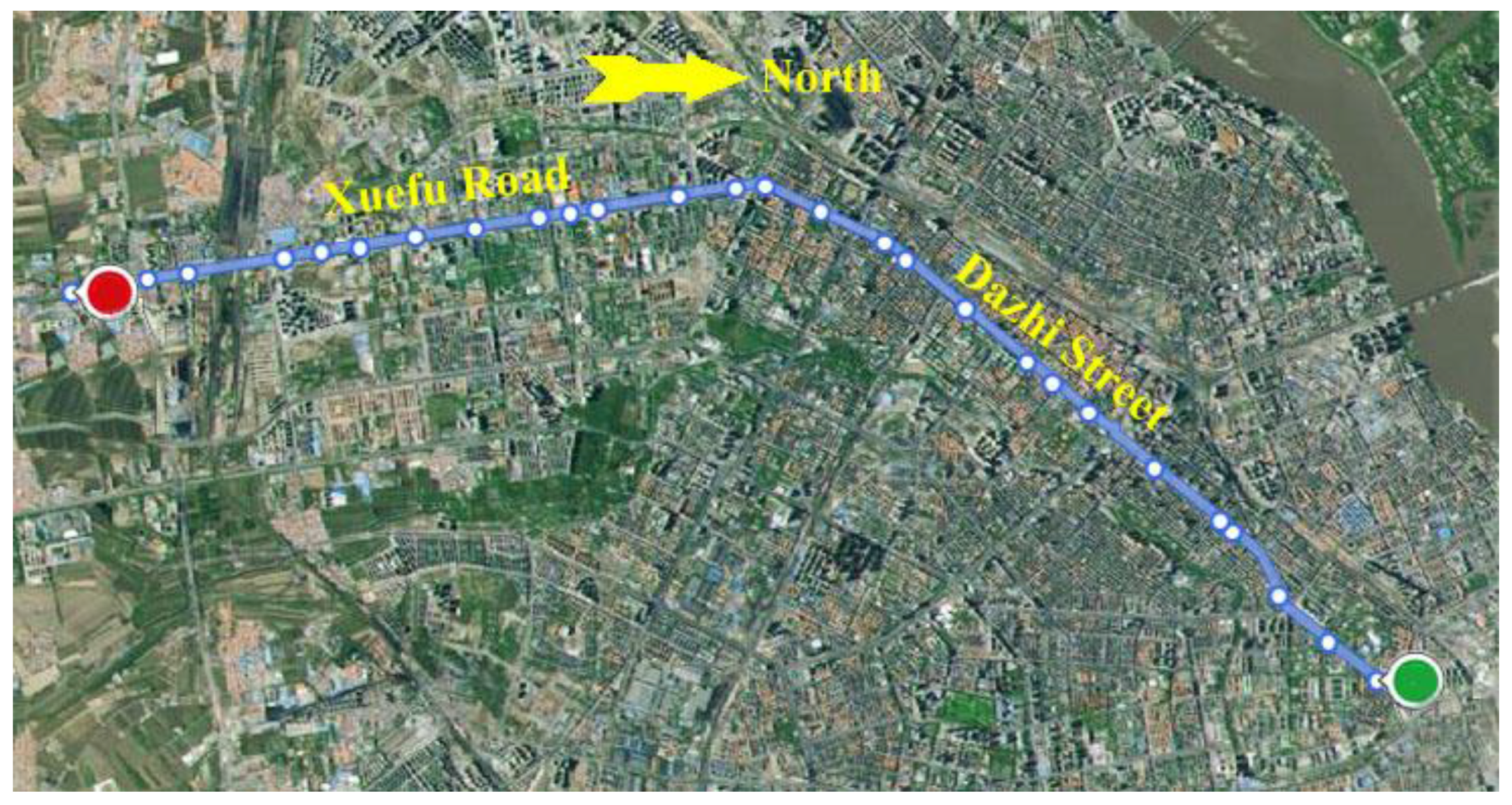
The bus line selected is Route 104 in Harbin, which travels along the east–west axis of the city, with a total of 28 stops. The route map is presented in Figure 1. Route 104 travels on the Xuefu Road and Dazhi Street, which are the busiest roads in rush hour in Harbin. Additionally, the bus line coincides with the metro line No.1, the only subway open in Harbin at present. On account of the traffic pressure and large transit demand, Route 104 provides relatively lower service levels, especially at rush hour. The importance of the line and the low level of service are the reasons why Route 104 is studied.

Figure 1. The route map of Line 104 in Harbin.

Figure 1. The route map of Line 104 in Harbin.

3.2. Data Description

The studied data is collected in March 2015, totally 22 days excluding weekdays. Three tables are recorded by bus GPS: “T_JK_LEAVESTATION” and “T_JK_ARRIVESTATION” store information about buses leaving and arriving at stations, respectively. While “T_JK_FULLGPSDATA” records all the information, including real-time location, direction, speed, status, etc. For a bus, a piece of GPS data is recorded every 15 seconds. Positioning errors exist like other AVL systems, but the algorithms of the position calibrator, such as map matching, are not necessary because the time arriving at or leaving stations is recorded precisely and that is enough for this research. “T_JK_LEAVESTATION” is analyzed only because it has recorded enough data used for the research. Table 1 below shows some useful fields used.

The column “O_LINENAME” is the number of the route; “O_BUSNAME” is a unique identification of a bus; “O_ARRIVEDATE” and “O_ARRIVETIME” are the actual arrival date and time for that bus at that stop; while “O_LEAVEDATE” and “O_LEAVETIME” are the actual departure date and time for that bus at that stop; “O_UP” indicates the orientation of a bus, “0” means that the bus is uplink, while “1” represents downlink.. The uplink of this route (from red point to the green point in Figure 1) is selected to be analyzed in this paper; and “O_STATIONNO” is the station number the bus leaves or arrives at.

Table 1. Information used in the research among the bus GPS data (sample data).

O_LINENAME	O_BUSNAME	O_ARRIVEDATE	O_ARRIVETIME	O_LEAVEDATE	O_LEAVETIME	O_UP	O_STATIONNO
104	3378	9 March 2015	08:27:39	9 March 2015	08:28:29	0	26
104	3389	9 March 2015	08:28:40	9 March 2015	08:29:10	0	13
104	3396	9 March 2015	08:22:29	9 March 2015	08:23:18	0	5
104	3377	9 March 2015	08:17:02	9 March 2015	08:21:17	0	22
104	3377	9 March 2015	08:21:18	9 March 2015	08:21:18	0	23
104	3377	9 March 2015	08:21:19	9 March 2015	08:23:01	0	24
104	3412	9 March 2015	08:28:34	9 March 2015	08:28:48	0	10
104	3396	9 March 2015	08:28:34	9 March 2015	08:29:02	0	8

Table 1. Information used in the research among the bus GPS data (sample data).

O_LINENAME	O_BUSNAME	O_ARRIVEDATE	O_ARRIVETIME	O_LEAVEDATE	O_LEAVETIME	O_UP	O_STATIONNO
104	3378	9 March 2015	08:27:39	9 March 2015	08:28:29	0	26
104	3389	9 March 2015	08:28:40	9 March 2015	08:29:10	0	13
104	3396	9 March 2015	08:22:29	9 March 2015	08:23:18	0	5
104	3377	9 March 2015	08:17:02	9 March 2015	08:21:17	0	22
104	3377	9 March 2015	08:21:18	9 March 2015	08:21:18	0	23
104	3377	9 March 2015	08:21:19	9 March 2015	08:23:01	0	24
104	3412	9 March 2015	08:28:34	9 March 2015	08:28:48	0	10
104	3396	9 March 2015	08:28:34	9 March 2015	08:29:02	0	8

4. Headway Performance Evaluation

The headway of buses is defined as the time interval between two contiguous buses arriving at the same station. It is one of the important indicators reflecting the transit network service level. The longer the headway is, the longer the waiting time of passengers, while too short a headway would lead to waste of public resources. In this section, the original GPS data, after preprocessed, are used to analyze spatial-temporal characteristics of the headway performance of Route 104 in Harbin. Then, a tatistics-based method to identify the abnormal headway (too long or too short) is proposed.

4.1. Data Preprocessing

For the purpose of this research, several new tables need to be created for convenience of analysis. For each stop, an arrival information table (see Table 2) should be built and sorted by arrival time to analyze the headway and dwell time. For each bus, a running information table sorted by station number, as shown in Table 3, is necessary. Additionally, the spatial neighbor relation of stops and the temporal neighbor relation of buses also needs to be determined.

Table 2. The arrival information table of stop 15 (sample data).

O_LINENAME	O_BUSNAME	O_ARRIVEDATE	O_ARRIVETIME	O_LEAVEDATE	O_LEAVETIME	O_STATIONNO
104	3389	9 March 2015	05:50:08	9 March 2015	05:50:42	15
104	3380	9 March 2015	05:54:48	9 March 2015	05:55:20	15
104	3412	9 March 2015	06:08:01	9 March 2015	06:08:02	15
104	3396	9 March 2015	06:10:17	9 March 2015	06:10:54	15
104	3382	9 March 2015	06:12:03	9 March 2015	06:13:28	15
104	3401	9 March 2015	06:20:20	9 March 2015	06:21:03	15

Table 2. The arrival information table of stop 15 (sample data).

O_LINENAME	O_BUSNAME	O_ARRIVEDATE	O_ARRIVETIME	O_LEAVEDATE	O_LEAVETIME	O_STATIONNO
104	3389	9 March 2015	05:50:08	9 March 2015	05:50:42	15
104	3380	9 March 2015	05:54:48	9 March 2015	05:55:20	15
104	3412	9 March 2015	06:08:01	9 March 2015	06:08:02	15
104	3396	9 March 2015	06:10:17	9 March 2015	06:10:54	15
104	3382	9 March 2015	06:12:03	9 March 2015	06:13:28	15
104	3401	9 March 2015	06:20:20	9 March 2015	06:21:03	15

Table 3. The running information table of bus 3373 (sample data).

O_LINENAME	O_BUSNAME	O_ARRIVEDATE	O_ARRIVETIME	O_LEAVEDATE	O_LEAVETIME	O_STATIONNO
104	3373	9 March 2015	07:11:36	9 March 2015	07:11:36	1
104	3373	9 March 2015	07:11:43	9 March 2015	07:12:00	2
104	3373	9 March 2015	07:12:55	9 March 2015	07:13:44	3
104	3373	9 March 2015	07:14:16	9 March 2015	07:15:24	4
104	3373	9 March 2015	07:17:18	9 March 2015	07:18:00	5
104	3373	9 March 2015	07:19:07	9 March 2015	07:19:48	6
104	3373	9 March 2015	07:21:58	9 March 2015	07:22:42	7
104	3373	9 March 2015	07:23:20	9 March 2015	07:23:56	8

Table 3. The running information table of bus 3373 (sample data).

O_LINENAME	O_BUSNAME	O_ARRIVEDATE	O_ARRIVETIME	O_LEAVEDATE	O_LEAVETIME	O_STATIONNO
104	3373	9 March 2015	07:11:36	9 March 2015	07:11:36	1
104	3373	9 March 2015	07:11:43	9 March 2015	07:12:00	2
104	3373	9 March 2015	07:12:55	9 March 2015	07:13:44	3
104	3373	9 March 2015	07:14:16	9 March 2015	07:15:24	4
104	3373	9 March 2015	07:17:18	9 March 2015	07:18:00	5
104	3373	9 March 2015	07:19:07	9 March 2015	07:19:48	6
104	3373	9 March 2015	07:21:58	9 March 2015	07:22:42	7
104	3373	9 March 2015	07:23:20	9 March 2015	07:23:56	8

For each bus stop, the headway between two buses equals to the arrival time of the following bus minus the arrival time of the front bus in the arrival information table. It is crucial to eliminate any erroneous results causing by GPS data leakage, clock errors, and other systematic errors. Since the buses travels along fixed routes and only time and bus stations are concerned in the research, just systematic errors are considered. Three times the standard deviation is recognized as the limiting error for $p\left(-3\sigma <\Delta <3\sigma \right)=0.993$. Thus the erroneous results are cleaned under this standard.

4.2. Spatial-temporal Characteristics Analysis

For measuring headway regularity, the schedule adherence index proposed by The Second Edition Transit Capacity and Quality of Service Manual (TCQSM 2^nd) is used in this paper, which is particularly applicable for high frequency transit service. The index is calculated as follows [26]

$$c_{vh}=\frac{standarddeviationofheadwaydeviations}{meanscheduledheadway}$$

(1)

where c_vh is the coefficient of variation of headways, and the headway deviation is the difference between the actual headway and the scheduled headway. The parameter c_vh reflects the variation of headways and the transit service reliability of a bus route at a certain station. According to the value of c_vh, the transit service is divided into five levels, as shown in Table 4:

Table 4. The level of transit service classification.

Levels	A	B	C	D	E	F
Value ranges	0.00~0.21	0.22~0.30	0.31~0.39	0.40~0.52	0.53~0.74	0.75~1

Table 4. The level of transit service classification.

Levels	A	B	C	D	E	F
Value ranges	0.00~0.21	0.22~0.30	0.31~0.39	0.40~0.52	0.53~0.74	0.75~1

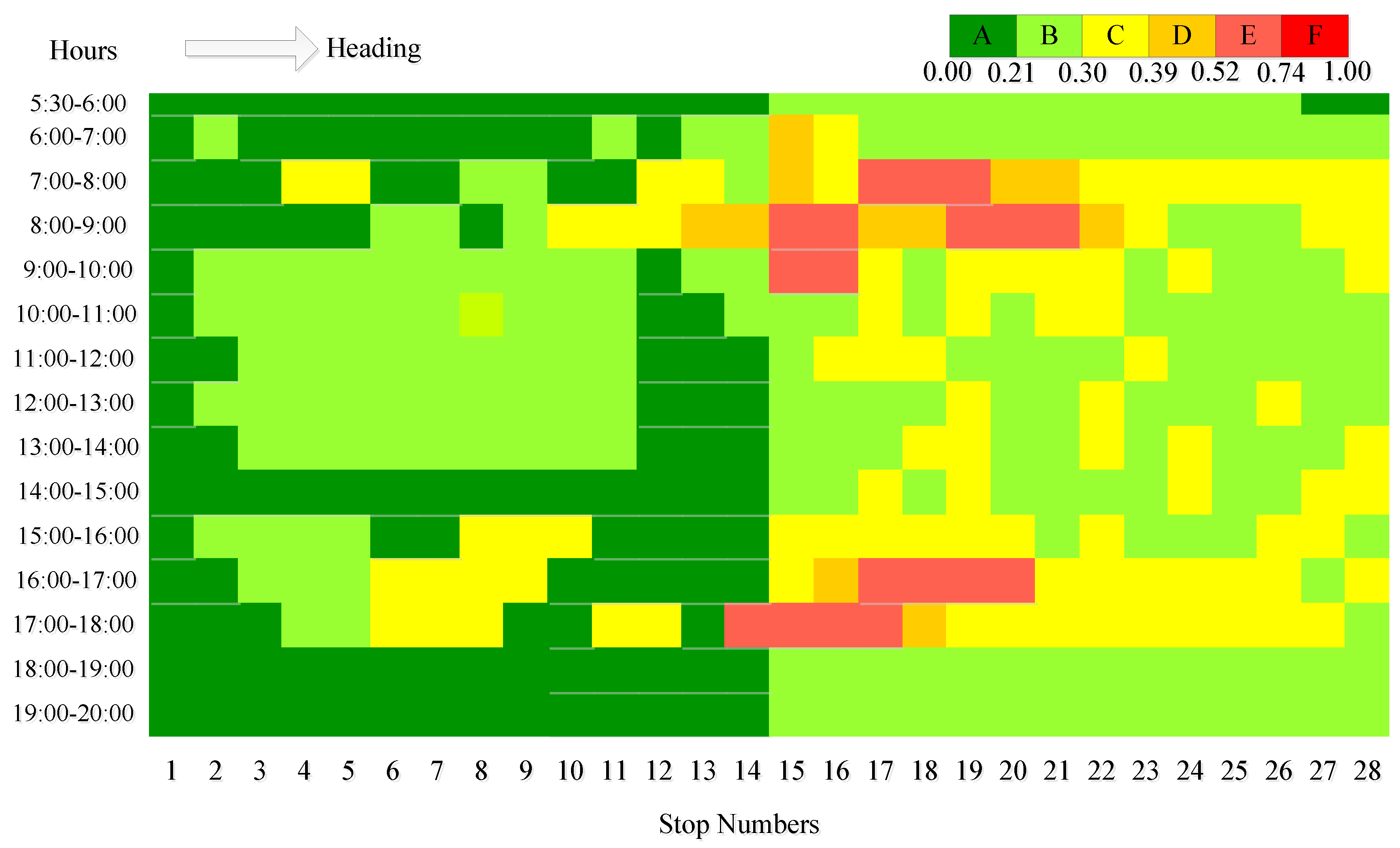
Level A means that the headway of the station is stable and a high-quality transit service is provided. While level F implies the service level is very low on account of a wildly fluctuating headway.

Figure 2 shows the temporal and spatial distributions of the headway service level obtained from the bus GPS data. The time frame is set from 5:30 to 20:00 including morning and evening rush hours and off-peak hours. The service levels are depicted by a range of colors, from green to red, corresponding to level A to level F.

Figure 2. Temporal and spatial distributions of the headway service level of Route 104.

Figure 2. Temporal and spatial distributions of the headway service level of Route 104.

The level of stop No.1 remains green all the time in Figure 2 because it is the origin stop with a fixed departure interval. Obviously it can be found in the figure that a lower level of services appears at 7:00 to 10:00 and 16:00 to 18:00, which coincides with rush hour, mostly. This suggests the temporal characteristic of bus headway, while in space, namely stations, the service level of stop No.14 to No.21 drops to level E in rush hours. These stations are all along the West Dazhi Street, which is one of the most crowded roadways in Harbin. In addition, it is clear that the service level decreases firstly (until stop 21) and increases subsequently (to the end) from the origin station to the terminal station in the same period, especially peak hours. It contains the formation process and the dissipation process along the bus line.

This is an evaluation of bus headway and service level. To find the reason why the service level goes down, it is necessary to identify the abnormal headways with a criterion to define the too long headways and the too short headways.

4.3. Abnormal Headway Identification

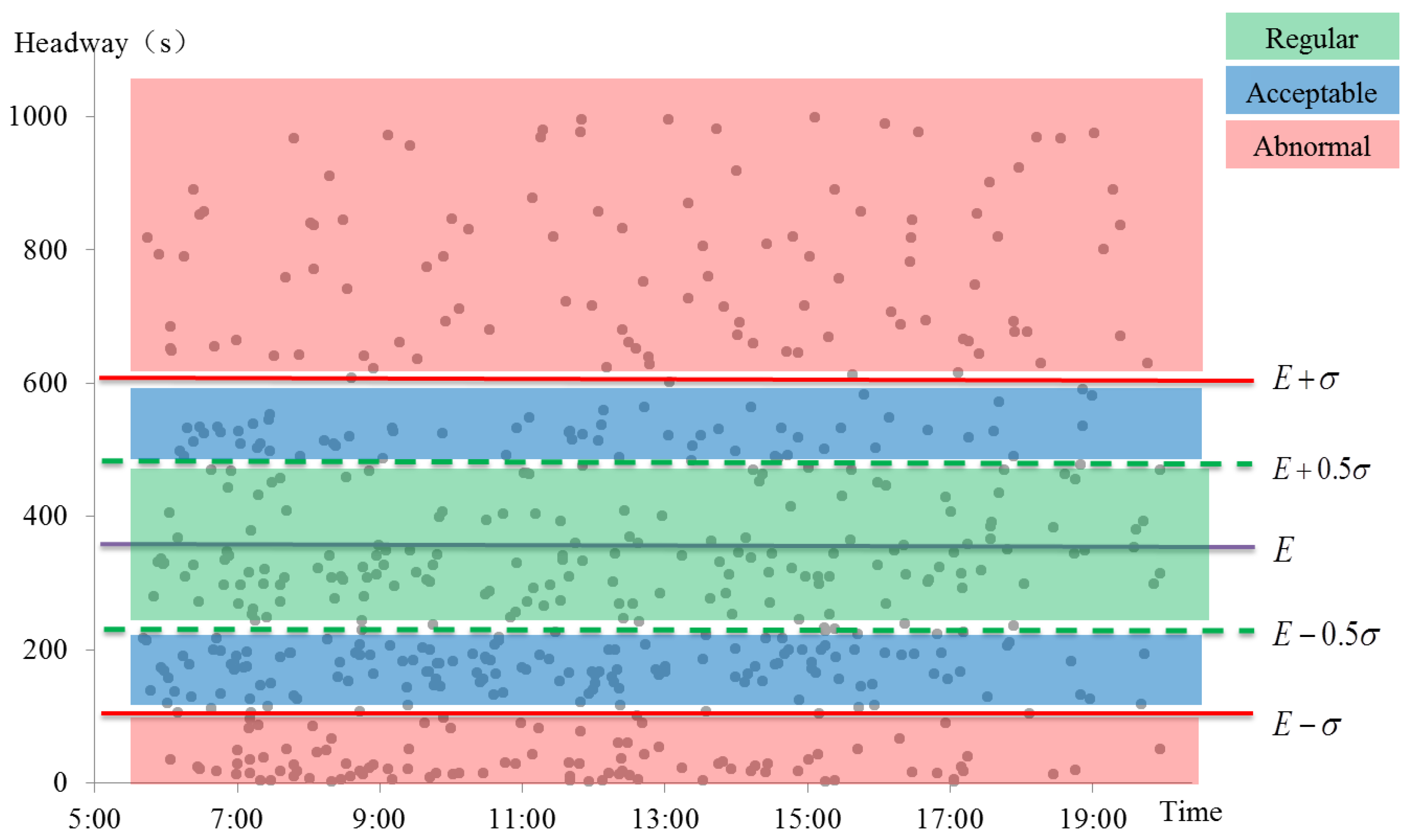
Abnormal headways, including longer or shorter headways relative to scheduled headway, are the leading cause reducing service levels, while, in consideration of normal errors of headway, such as driving habits of bus drives and normal travel fluctuations, the reference value to identify the abnormal headways is not supposed to be the scheduled headway (departure interval at the origin station). It is more reasonable to set the expectation of the headways at a stop as the reference value in statistics. Another statistical parameter, variance, reflects the discreteness of a dataset. Thus, the expectation and the variance define the normal range of the headway dataset of a stop statistically.

Figure 3 illustrates the method to identify the abnormal headways, taking stop No.15 as an example. The expectation (E) of headways in 22 days of stop No.15 is 348 seconds, and the standard deviation (σ) of these headways is 258 seconds. The headways are divided into three groups as shown in Figure 3. Data ranging from (E − 0.5σ)(219s) to (E + 0.5σ)(477s) are recognized as regular headways, which are in the green area between two green dashed lines in the figure. Data ranging from (E − σ)(90s) to (E + σ)(606s) (excluding the regular headways) are within the normal discrete range, and these observations are acceptable in statistics, as the blue areas in the graph. As for the red areas, headways in these areas beyond the normal fluctuations and are identified as the abnormal data. Headways less than (E − σ) are too short and ones more than (E + σ) are too long.

Figure 3. Abnormal headway identification on stop No.15 of Route 104.

Figure 3. Abnormal headway identification on stop No.15 of Route 104.

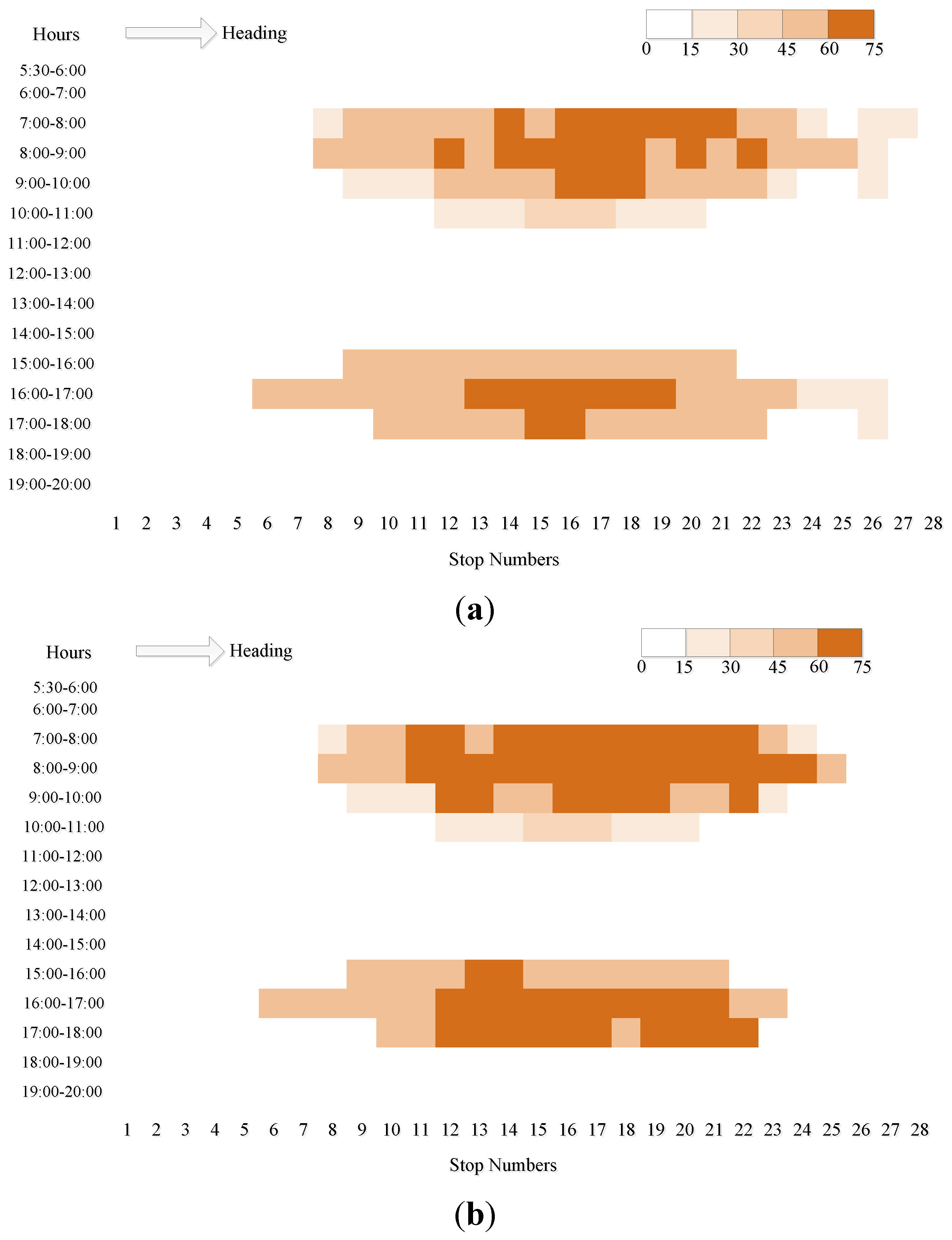
Figure 4. (a) Distributions of too short headways of Route 104; and (b) distributions of too long headways of Route 104.

Figure 4. (a) Distributions of too short headways of Route 104; and (b) distributions of too long headways of Route 104.

The results of abnormal headways identification at each stops of Route 104 are shown in Figure 4. Too short headways and too long headways are pictured in Figure 4a,b, respectively. Obviously, the distributions of abnormal headway frequency and the service level are similar. However, what is interesting is that the frequencies of too short headways and too long headways are very close to each other. This is logical because when a too short headway takes place, two or more buses arrive together and one of them is ahead or behind its schedule causing the fixed departure interval at the origin station. Thus, the waiting time of passengers at the stop increases and a too long headway occurs, consequently. In fact, the too short headways give rise to a phenomenon called bus bunching. The most serious drawback of bus bunching is misallocation and waste of public transportation capacity. Once two or more buses form a bunch, the front bus is more likely to be crowded for collecting more passengers while fewer passengers are left for the following bus for shorter headway. Moreover, there will be a long interval for the next bus arriving at this stop. Thus, the passenger’s waiting time is increased and more traffic demand is accumulated, which tends to increase thedelay of the bus and cause another bunching. This is the reason for the lower transit service level.

5. Causes of Bus Bunching Analysis

Bus bunching is a phenomenon resulting from too short headways. For the purpose of regular headways and improving transit service level, it is crucial to find the causes of bus bunching.

5.1. Causes Identification by Association Mining

It has been analyzed that the reasons why bus bunching happened included two aspects, travel time between stops and passenger numbers (boarding and alighting) at stops [25]. The latter can be measured by the dwell time at stops for uniformity. To find more specific reasons in time and space to solve this problem, association mining is used in this research. Before that, states of events should be defined in advance.

Using the method of bus bunching identification mentioned above, too long/too short dwell time and travel time could also be recognized. Thus, when a bus arrives at a stop, there is a state set S*.

$$S*=\{Sdwelltime,Straveltime,Sbunching\}$$

(2)

where Sdwellitme and Straveltime represent the states of dwell time and travel time, respectively, containing three optional states: too long, too short, and normal. Sbunching has two optional states: bunching or not, indicating the state of bus bunching.

Thus, Apriori algorithm is applied to mine the association among Sdwellitme, Straveltime, and Sbunching for each bus and each stop. Two measures, support and confidence, are used to indicate the quality of an association rule. Six causes are identified according to the results of association mining, as shown in Table 5.

Table 5. Relative degree of importance for pairwise comparisons.

Causes	Description
A	Front bus—long dwell time at current stop
B	Front bus—long travel time from previous stop to current stop
C	Front bus—late departure from previous stop
D	Following bus—short dwell time or stay time at current stop
E	Following bus—short travel time from previous stop to current stop
F	Following bus—early departure from previous stop

Table 5. Relative degree of importance for pairwise comparisons.

Causes	Description
A	Front bus—long dwell time at current stop
B	Front bus—long travel time from previous stop to current stop
C	Front bus—late departure from previous stop
D	Following bus—short dwell time or stay time at current stop
E	Following bus—short travel time from previous stop to current stop
F	Following bus—early departure from previous stop

The six causes do not happened separately in most cases. One or a combination could cause the phenomenon of bus bunching, thus it is necessary to determine the weight of each cause.

5.2. Causes Weight Analysis Using AHP

The Analytic Hierarchy Process (AHP), proposed by Saaty in the 1970s [27], is an important decision analysis theory in operational research. It can solve semi-qualitative and semi-quantitative problems in a quantitative way. The basic principle of AHP is sorting, namely, determining the optimal sorting of alternative schemes to make decisions. Specifically, a decision problem is regarded as a system affected by various factors in the AHP. These interrelating and interdependent factors can be divided into several hierarchies according to the subordination, which is called the hierarchical structure model. Then, the AHP makes comparisons between every two factors and gets the sort order by weight of all factors to help with decision-making. The AHP, embedded data analysis, is used in this research to determine the weights of the six causes of bus bunching. The main steps of the method are detailed as follows.

(1) Structure of judgment matrix

The judgment matrix describes the relative importance between any two of the six causes, which is the key step in AHP. The scale used is shown in Table 6 when performing pairwise comparisons [28]. For example, for a judgment matrix A = [a_ij], a_ij = 5 means that factor i is of essential or strong importance compared to factor j.

Table 6. Relative degree of importance for pairwise comparisons.

Comparative Importance	Description
1	Equally importance
2	Intermediate between equal and weak
3	Weak importance of one over another
4	Intermediate between weak and strong
5	Essential or strong importance
6	Intermediate between strong and demonstrated
7	Demonstrated importance
8	Intermediate between demonstrated and absolute
9	Absolute or extreme importance

Table 6. Relative degree of importance for pairwise comparisons.

Comparative Importance	Description
1	Equally importance
2	Intermediate between equal and weak
3	Weak importance of one over another
4	Intermediate between weak and strong
5	Essential or strong importance
6	Intermediate between strong and demonstrated
7	Demonstrated importance
8	Intermediate between demonstrated and absolute
9	Absolute or extreme importance

Although it is considered to be reasonable to sorting out nine grades, the subjectivity exists more or less when making a judgment. A judgment method, which is completely based on the objective data, is proposed in this paper.

Taking No.15 station as an example, the bus bunching occurred 392 times in the research period according to the data analysis. The total number 392 is divided into nine groups and presented in the value’s descending order, as shown in Table 7.

Table 7. The divided groups of total numbers.

Group Numbers	1	2	3	4	5	6	7	8	9
Ranges	348.8–392	305.2–348.8	261.6–305.2	218–261.6	174.4–218	130.8–174.4	87.2–130.8	43.6–87.2	0–43.6

Table 7. The divided groups of total numbers.

Group Numbers	1	2	3	4	5	6	7	8	9
Ranges	348.8–392	305.2–348.8	261.6–305.2	218–261.6	174.4–218	130.8–174.4	87.2–130.8	43.6–87.2	0–43.6

Since one, or a combination, of the six causes could lead to bus bunching, and it is hard to make a detailed distinction, an exclusive method is proposed in this paper. Bus bunching happened 290 times without cause A, that is, the five other causes (one or a combination) could lead to 290 times the bus bunching. The more times bus bunching happened without a cause, the less important the cause is. The results of the “exclusion” method are presented in Table 8.

Table 8. The results of exclusive method.

Group Numbers	Bus Bunching Times	Groups
Exclusion of cause A	290	3
Exclusion of cause B	330	2
Exclusion of cause C	98	7
Exclusion of cause D	188	5
Exclusion of cause E	341	2
Exclusion of cause F	278	3

Table 8. The results of exclusive method.

Group Numbers	Bus Bunching Times	Groups
Exclusion of cause A	290	3
Exclusion of cause B	330	2
Exclusion of cause C	98	7
Exclusion of cause D	188	5
Exclusion of cause E	341	2
Exclusion of cause F	278	3

The comparative importance between cause A and cause B equals to one plus the difference of between the group numbers, namely, (3 − 2) + 1 = 2. More times happened without cause B, so cause B is less important than cause A. Thus, the importance of A to B is 2 and B to A is 1/2. Then the judgment matrix can be structured as follows.

$$A=\left[\begin{array}{cccccc}1& 2& \raisebox{1ex}{$1$}\!\left/ \!\raisebox{-1ex}{$5$}\right.& \raisebox{1ex}{$1$}\!\left/ \!\raisebox{-1ex}{$3$}\right.& 2& 1\\ \raisebox{1ex}{$1$}\!\left/ \!\raisebox{-1ex}{$2$}\right.& 1& \raisebox{1ex}{$1$}\!\left/ \!\raisebox{-1ex}{$6$}\right.& \raisebox{1ex}{$1$}\!\left/ \!\raisebox{-1ex}{$4$}\right.& 1& \raisebox{1ex}{$1$}\!\left/ \!\raisebox{-1ex}{$2$}\right.\\ 5& 6& 1& 3& 6& 5\\ 3& 4& \raisebox{1ex}{$1$}\!\left/ \!\raisebox{-1ex}{$3$}\right.& 1& 4& 3\\ \raisebox{1ex}{$1$}\!\left/ \!\raisebox{-1ex}{$2$}\right.& 1& \raisebox{1ex}{$1$}\!\left/ \!\raisebox{-1ex}{$6$}\right.& \raisebox{1ex}{$1$}\!\left/ \!\raisebox{-1ex}{$4$}\right.& 1& \raisebox{1ex}{$1$}\!\left/ \!\raisebox{-1ex}{$2$}\right.\\ 1& 2& \raisebox{1ex}{$1$}\!\left/ \!\raisebox{-1ex}{$5$}\right.& \raisebox{1ex}{$1$}\!\left/ \!\raisebox{-1ex}{$3$}\right.& 2& 1\end{array}\right]$$

(2) Assessment of the consistency of pairwise judgments

The judgment matrix A = [a_ij] meets consistency when satisfying the following condition

$$a_{ij}{a}_{jk}=a_{ik}i,j,k=1,2,\mathrm{...},n$$

(3)

Obviously, the pairwise judgments between every two factors are transmissible and the judgment thinking is consistent when the given matrix A satisfies the consistency. Thus, assessing the consistency of pairwise judgments is necessary to ensure the accuracy.

It has been proved that necessary and sufficient conditions for a consistant reciprocal matrix A = (a_ij)_{n × n} is that the maximum eigenvalue (λ_max) of A equals n. Saaty defined a consistency index (CI) to measure the degree of inconsistency [28].

$$CI=\frac{{\lambda }_{\max }-n}{n-1}$$

(4)

Technically, perfect consistency implies CI = 0. However, perfect consistency is seldom achieved. So, Saaty proposed a mean random consistency index (RI) to assess the consistency of pairwise judgments together with CI. The RI is obtained as follows:

For a certain n, Saaty structured a reciprocal matrix A’ randomly. The elements of A’ were selected among 1, 2, ..., 9, 1/2, 1/3, ..., 1/9. When the samples are large enough, 500 for example, the average value of the maximum eigenvalues of A’ is calculated as ${\lambda }_{max}^{\text{'}}$, and

$$RI=\frac{{\lambda }_{\max }^{\text{'}}-n}{n-1}$$

(5)

Saaty presented the values of RI for n valued from 1 to 9, as shown in Table 9 [28].

Table 9. Values of the mean random consistency index (RI).

n	1	2	3	4	5	6	7	8	9
RI	0	0	0.58	0.90	1.12	1.24	1.32	1.41	1.45

Table 9. Values of the mean random consistency index (RI).

n	1	2	3	4	5	6	7	8	9
RI	0	0	0.58	0.90	1.12	1.24	1.32	1.41	1.45

Then, the ratio of CI and RI is defined as the consistency ratio CR. It is consistency if CR < 0.1.

In this case, it can be obtained that λ_max = 6.09, CI $=\frac{{\lambda }_{\text{max}}-n}{n-1}=\frac{6.09-6}{6-1}=0.018$ and RI = 1.24, thus CR = CI/RI = 0.018/1.24 = 0.015 < 0.1. The results show that the judgment matrix is consistency.

(3) Computation of the relative weights

So far the relative weights can be gained by the eigenvector of the maximum eigenvalue and the results of stop No.14 to No.21, which are of lower service level, are shown in Table 10.

Table 10. The results of causes weight analysis.

Causes	Weights
	No.14	No.15	No.16	No.17	No.18	No.19	No.20	No.21
A: Front bus—long dwell time at current stop;	0.116	0.097	0.11	0.075	0.054	0.042	0.049	0.039
B: Front bus—long travel time from previous stop to current stop;	0.298	0.232	0.221	0.212	0.265	0.301	0.236	0.198
C: Front bus—late departure from previous stop;	0.39	0.460	0.516	0.592	0.56	0.566	0.601	0.632
D: Following bus—short dwell time at current stop.	0.049	0.057	0.068	0.023	0.059	0.031	0.051	0.044
E: Following bus—short travel time from previous stop to current stop;	0.065	0.057	0.04	0.048	0.02	0.022	0.015	0.044
F: Following bus—early departure from previous stop;	0.082	0.097	0.045	0.05	0.042	0.038	0.048	0.043

Table 10. The results of causes weight analysis.

Causes	Weights
	No.14	No.15	No.16	No.17	No.18	No.19	No.20	No.21
A: Front bus—long dwell time at current stop;	0.116	0.097	0.11	0.075	0.054	0.042	0.049	0.039
B: Front bus—long travel time from previous stop to current stop;	0.298	0.232	0.221	0.212	0.265	0.301	0.236	0.198
C: Front bus—late departure from previous stop;	0.39	0.460	0.516	0.592	0.56	0.566	0.601	0.632
D: Following bus—short dwell time at current stop.	0.049	0.057	0.068	0.023	0.059	0.031	0.051	0.044
E: Following bus—short travel time from previous stop to current stop;	0.065	0.057	0.04	0.048	0.02	0.022	0.015	0.044
F: Following bus—early departure from previous stop;	0.082	0.097	0.045	0.05	0.042	0.038	0.048	0.043

Based on the analysis results, “Cause C: Front bus—late departure from previous stop” plays an obvious role to arouse bus bunching. The front bus leaving late at the previous stop implies that abnormal headway emerges at the stop before the previous stop. Meanwhile, this may be related to the upstream stops. This finding confirms that “there is a positive feedback loop that causes undesirable bunching” [29]. Additionally, “B: Front bus—long travel time from previous stop to current stop” is the second most important reason. Long travel time means bad traffic on the road. This indicates that the traffic condition is a key factor to bus bunching. Among the six causes, the front bus has a greater effect on bus bunching than the following bus. These weighted causes could influence the improvement measures significantly.

6. Conclusions

This paper studies the transit headways using bus GPS data in Harbin. The headway performance of the selected Route 104 is evaluated and it is found that lower transit service levels emerge in rush hour, especially at stop No. 14 to No. 21. Statistically, a method to identify the abnormal headways is proposed based on the two parameters: expectation and standard deviation. Deeply, the association mining is applied to the spatial-temporal data and six causes of bus bunching are revealed, including dwell time of the front and following buses, travel time of the front and following buses, and the previous influences of these buses.

Through data analysis, it is found that these causes are often combined with each other. In order to obtain a better understanding of the causes and conduct the effective improvement measures, the AHP, embedded data analysis, is used. The judgment matrix is structured by the proposed “exclusion” method. The results indicate that the previous influences of buses are the most serious cause of bus bunching, and bus bunching is affected by the front bus more than the following bus. Furthermore, travel time is significant to maintain the regular headway. These findings are significantly helpful to improve the transit service level.

The advantages of the proposed approach lie in two points. On the one hand, the causes of bus bunching could be found by data mining, but the influence mechanism remains unclear as one or a combination of these causes could lead to bus bunching. Thus, the AHP is embedded to determine the weight of each cause, which is of great significance in proposing measures to improve bus service. On the other hand, a data-based approach to structuring the judgment matrix in AHP is used, which makes the results of pairwise judgments more convincing.

Additionally, some weaknesses of this work exist and there are some problems remaining unsolved. Firstly, the dwell time at a station is regarded as the transit demand in the study. This is an indirect approximate method on account of the insufficient data. If possible, it is better to use bus IC data to analyze the number of passengers boarding/alighting at each stop and measure the impact on the bus running time. Secondly, the data mining method used in this work only includes association analysis because it is simple and effective enough to get the expected results. For more accurate results and extensive range of application, other techniques, such as machine learning approaches, are also encouraged. Thirdly, the method proposed is applied to the case that only one bus line exists. To solve practical problems effectively, multiple bus line analyses should be done and the interaction of bus lines and the public transportation transfer also needs to be considered carefully. Lastly, although passive irregular headways have some negative effects on the transit service, they could be beneficial to meet the dynamic transit demand by being controlled actively. For example, bus bunching could be very helpful when the demand is beyond the capacity of a bus. How to eliminate the adverse bus bunching and produce beneficial bus bunching is one of the future research directions.