Weather Conditions, Weather Information and Car Crashes

Abstract

Road traffic safety is the result of a complex interaction of factors, and causes behind road vehicle crashes require different measures to reduce their impacts. This study assesses how strongly the variation in daily winter crash rates associates with weather conditions in Finland. This is done by illustrating trends and spatiotemporal variation in the crash rates, by showing how a GIS application can evidence the association between temporary rises in regional crash rates and the occurrence of bad weather, and with a regression model on crash rate sensitivity to adverse weather conditions. The analysis indicates that a base rate of crashes depending on non-weather factors exists, and some combinations of extreme weather conditions are able to substantially push up crash rates on days with bad weather. Some spatial causation factors, such as variation of geophysical characteristics causing systematic differences in the distributions of weather variables, exist. Yet, even in winter, non-spatial factors are normally more significant. GIS data can support optimal deployment of rescue services and enhance in-depth quantitative analysis by helping to identify the most appropriate spatial and temporal resolutions. However, the supportive role of GIS should not be inferred as existence of highly significant spatial causation.

1. Introduction

1.1. Background

Road traffic safety is the result of a complex interaction of technical, environmental and behavioural factors, and different causes behind road vehicle crashes require different measures to reduce their impacts. Some of the causes have a behavioural background often steered by attitudes and social norms. Measures may include speed limit enforcement and awareness campaigns. Other causes have a technical-physical nature which can be managed by means of monitoring the physical condition of roads and vehicles and by imposing minimum standards. Despite the large differences between the causes, they have in common that humans can have some degree of control over them as individuals or institutions.

For weather related hazards, this is much less the case. Therefore, the main counter measures are better preparedness and maximizing adaptability (departure time, route, mode choice). To some extent, the technical conditions and standards of the involved vehicles and infrastructure matter, but implemented designs cannot be changed overnight, leaving last-minute measures, such as variable speed limits, road clearing and increased emergency response as the only options. However, decisions on how, when and where to implement these measures are largely a matter of the aforementioned preparedness. As preparedness is the key factor with respect to bad road weather conditions, weather forecasts play an important role in reducing weather related crashes, even though the effectiveness of road weather services depends on many factors of which forecast quality is only one [1,2,3].

Throughout the article, the terms “car crash” and “road vehicle crash” will be used. In many studies, including this one, also other (motorized) road vehicles are included in the analysis. Passenger cars are nevertheless by far the largest sub-group.

1.2. Aim

In this study, we aim to assess how strongly the variation in daily crash rates associates with weather conditions in Finland, a country characterised by heavy winter road conditions. On the one hand, this is relevant for raising the effectiveness of road weather warning services, while on the other hand, it may help rescue and medical services to project the number of emergencies in designated regions in case weather forecasts foresee bad conditions for road transport. Lastly, from an academic point of view, the analysis could help to obtain a more precise understanding of the relative contribution of different weather characteristics in the resulting weather generated hazards for road transport, and the sensitivity of apparent crash rates regarding the intensity of relevant weather characteristics—separately and jointly.

We first discuss the causes of car crashes with a particular focus on weather-related causes, and alternative research approaches in Section 2. Section 3 presents the data used in the study. In Section 4, we depict the evolution and spatial variation of crash rates in Finland and show that location matters, not in the sense of unfavourable local road lay-out or landscape, but through spatial differences in intensity of bad weather. In Section 5, we introduce a statistical model of crash rate sensitivity. According to the modelling results, weather conditions have to deteriorate quite significantly before notable rises in crash rates occur.

We intend to show that with an appropriate level of spatial and temporal resolution, this kind of crash projection tool can assist in day-ahead rescue preparedness, response and road clearance, and help to improve the road weather information services. Geographically referenced information is helpful for quick identification and communication of localized accident risks. Georeferenced data can also enhance in-depth quantitative analysis, as they help to identify the most appropriate spatial and temporal resolutions for the estimation input data and for segmentations in the analysis. However, this highly supportive role of georeferenced data should not be confused with inferences that a lot of spatially defined causation is involved. This study tries to shed some light on the significance of spatial causation for the effects of influence factors of crash rates, given the spatial scales considered.

2. Approaches in Analysis of Road Traffic Sensitivity to Weather—A Literature Review

There are several strands in the literature on the factors behind road vehicle crashes, for instance, studies dealing with intoxication of drivers, weather conditions, road system quality and speeding and speed limit enforcement [4,5]. An important distinction between approaches is formed by the prime orientation of the analysis, i.e. the driver, the vehicle, a combination of driver and vehicle, the infrastructure (and its immediate environment), (weather) events, accident hotspots, and injury vs. accident [6,7,8,9]. Furthermore, studies assessing the effectiveness of road transport safety policies need to be cross-cutting in order to avoid risks of erroneous attribution of effects to trends or measures [10,11,12].

An important distinction, also otherwise used in transport research, is between macroscopic and microscopic studies. In car crash research, microscopic studies are concerned with assessing the mechanisms directly leading to a particular accident or a particular type of accident. In research focusing on crashes caused by weather conditions, this approach is typically based on case studies of bad weather events [7]. Macroscopic studies deal with system level developments, and have—at least in principle—the ambition of taking into account all types of road safety factors and the road safety policy programmes as well. Key references for this approach are e.g. [13,14]. In practice, truly comprehensive analyses are often infeasible, and, therefore, many authors tend to focus on particular effects or relations, such as comparing crash rates between different regions or assessing trends in the rates in relation to selected explanatory macro-level variables, such as the size and composition of the car stock [15,16]. In addition, cross-country comparisons of road safety performance and measures can be attributed to this category [16,17]. Gitelman et al. [17] Shows, for the world’s best performing countries in terms of road safety, that only a few perform really well across the board, whereas most of these overall good performing countries appear to have some weak spots in their policy portfolio. Bergel-Hayat et al. [18] adopts a kind of meso-level approach comparing accident proneness by means of monthly data with respect to weather conditions in France, Greece and the Netherlands, while differentiating between road systems.

Geographically framed crash studies are a relatively young category of crash analysis. A principal distinction within this category of studies is whether the analysis is based on either the location of the crash or the residential location of the driver [19]. Another specific geographical-meteorological approach is to compare crashes in a certain area for two or a few identical time periods in different years but with distinctly different weather conditions [20].

Generally, it is very hard to merge the approaches based on the location of the crash with those based on residential location of the driver, as car crash statistics usually contain little or no information of the drivers. Insurance information in relation to crashes may contain more personal information, but it is usually parsimonious on the location of the crash, and observations tend to be truncated for smaller crashes. Crashes often also involve several drivers, who may well be from different (types of) areas, thereby creating categorisation problems in the residence based approach. Furthermore, drivers’ characteristics are largely based on non-spatial factors, such as age, health situation and driving experience. Truly spatial effects may occur to some extent in traits of driving behaviour and choice of car type through peer group mechanisms [21]. Yet, the spatial element remains weak in these peer pressure studies. All in all, the approach based on the location of the crash seems preferable, but the analysis should include information about the driver as much as possible.

Georeferenced databases on car crashes with simultaneous observations of traffic and weather conditions (in the crash region) are still rather scarce. Theofilatos et al. [22] review over 70 studies on crash rates in relation to driving conditions and find that approximately only 20 of them contain both traffic and weather data, among which five studies focus on the severity and 15 studies focus on the likelihood of the crash. The outcomes for crash severity and likelihood may not be the same. For example, intense precipitation increases the crash likelihood as compared to average conditions, but reduces severity as drivers adapt by reducing speed. Similar effects are reported for snowfall. Yet, Andrey et al. [23] indicate that the generality of the compensatory tendencies of frequency and severity in adverse weather conditions is still contested. Localized slipperiness or dense fog may increase severity as speed adjustment is much less systematic.

In fact, no single study manages to capture all significant factors. On the one hand, analysis of accident proneness requires simultaneous measurement of crash occurrence, traffic flow, road conditions, and weather circumstances at a fairly high spatial and temporal resolution. On the other hand, such an analysis would require diverse personal information about drivers (age, cumulated driving experience, general physical and mental condition, specific conditions (just) before the accident, possible intoxications, etc.) and vehicles (age, technical condition, presence of active safety technologies, easiness of driving) involved in the accidents. It is next to impossible to observe and merge all these variables simultaneously with limited resources. Simulation models enable to draw all insights together. However, desired spatial and temporal resolution and the choice between an infrastructure or driver vantage point will lead to quite different simulation models. New perspectives for fundamentally more comprehensive crash data sets are offered by the development of so-called “big data”, in which various large public (statistical) data sets are merged, for instance, with spatial-temporal data from mobile phones.

Studies in Norway and Finland find that weather conditions are the main cause in approximately 10% of crashes [24]. Andrey et al. [23] report a share of about 18% for Ontario (18.5% for crashes involving injuries and 16% for crashes involving fatalities). The same study investigated the effects of rainfall and snowfall on relative crash risk levels in selected Canadian cities, finding that snowfall has appreciably stronger effects than rainfall. In conjunction with other factors, adverse (but not necessarily extreme) weather can have a secondary contributing role—for instance, in the case of driver fatigue. Jaroszweski et al. [25] find a significant relationship between heavy rain and crash occurrence in selected urban areas in the UK.

Road traffic demand decreases during adverse weather [26], which attenuates the rise in accidents, while the extent of the decrease depends on the purpose of the trip (work, shopping, holiday, etc.). The structure of road traffic, the composition of drivers (by skill level) in the traffic, and the average degree of time pressure varies between days. Furthermore, Cools et al. [27] find that inferred deterrence effects of a given level of weather hazard depend also on the season and on the time scale (hours to days) at which responsiveness was assessed, as well as the kind of forecast weather and conformity between forecast and experienced weather.

The aforementioned studies do not, however, estimate the magnitude of the influence of the considered weather attributes, instead only the statistical significance of bad weather conditions is evidenced. Lin et al. [28] carry out a cluster analysis of observed crashes in a regional main road network and find that adverse weather circumstances do not discriminate much with respect to the other clustering factors listed. Instead, adverse weather increases the crash risk more or less across the board, implying that it is meaningful to conduct a focused analysis of the contribution of various weather variables to accident rates, even if a decomposition of interaction effects with other factors cannot be made. In this study, we go one step further and parametrize the influence of various characteristics of weather conditions, thereby enabling a more precise assessment of risky thresholds. The study by Brijs et al. [29] comes closest to the study discussed here. In [29] an integer autoregressive Poison regression model is applied to daily crash occurrence in three-differently sized and structured urban municipalities in the Netherlands. Yet, Brijs et al. [29] use only data of one year, whereas structural differences between the municipalities are captured by generic city dummies, rather than by e.g. variables capturing differences in the main road network and traffic composition. As in this study, Brijs et al. [29] use day-of-the-week dummies to capture typical variations (cycles) in traffic patterns.

3. Data

The causes of a particular crash can involve detailed situational factors which cannot be straightforwardly generalized. Therefore, when moving from individual crash analysis to statistical inference of crashes in a part of the system, only a few generalized indicators pertaining to conditions can be included, e.g. average age of the fleet, existence of technical inspection framework, etc. Table 1 presents categories of explanatory factors based on [4,19], and the variables included in this study.

The spatial resolution of the data used in the analysis is the EU NUTS-3 administrative level (Regions or “maakunta” in Finnish). Crash data, received from the Finnish Motor Insurers’ Centre (its traffic damage statistics) was merged with data on the road network per Region from the Finnish Road Administration (since then renamed Finnish Transport Agency). Each record states the number of crashes, casualties, injured, fatalities, type(s) of vehicles, and collision lay-out (on a crossing, head-on, etc.) for region r (=18) on day D in year Y (for 2000–2010). The data include only cases for which an insurer has been paying out compensation. The dataset includes also crashes without casualties, implying only damage to property has occurred. The dataset is subject to some degree of truncation as accidents with modest material damage and without injuries are not always registered (e.g., if the car owner(s) decide to refrain from claiming so as to retain cumulated premium benefits). Furthermore, crashes, including single car crashes, in which all involved drivers have violated the blood alcohol concentration limits are not included due to the lack of eligibility for insurance coverage.

Table 1. Types of factors influencing crash frequency and factors included in the model.

Types of Factors	Factors in the Model
Physical Environmental Conditions:
Resistance of the road surface (slipperiness due to frost, snowfall, heavy rain)	YES
Visibility (fog, dense precipitation, night/day)	YES
Strong cross-winds High wind speeds (aggravating precipitation effects)	NO* YES
Very low or very high temperatures	YES
Situational complexity (difficult terrain; distractive landscape features, etc)	NO
Road Quality:
Allowable speeds	NO**
Speed limit enforcement	NO
Separation of lanes	NO**
Traffic density	YES
Road side information systems	NO
Vehicle and Driver:
Condition of the car fleet (age, presence of technical condition inspection cycles, obligatory safety measures (e.g. winter tires), etc.)	NO
Share of non-experienced drivers	NO
Condition of the driver (intoxication, age, general condition)	NO
Experience level of driver(s); known or unknown route	NO
Number and conduct of co-travellers	NO
Information interface in the car	NO

* wind speed (without direction) is a variable in the model; ** the variable “share of motorways in the regional road system” refers to these aspects in a very generalized manner.

Table 1. Types of factors influencing crash frequency and factors included in the model.

Types of Factors	Factors in the Model
Physical Environmental Conditions:
Resistance of the road surface (slipperiness due to frost, snowfall, heavy rain)	YES
Visibility (fog, dense precipitation, night/day)	YES
Strong cross-winds High wind speeds (aggravating precipitation effects)	NO* YES
Very low or very high temperatures	YES
Situational complexity (difficult terrain; distractive landscape features, etc)	NO
Road Quality:
Allowable speeds	NO**
Speed limit enforcement	NO
Separation of lanes	NO**
Traffic density	YES
Road side information systems	NO
Vehicle and Driver:
Condition of the car fleet (age, presence of technical condition inspection cycles, obligatory safety measures (e.g. winter tires), etc.)	NO
Share of non-experienced drivers	NO
Condition of the driver (intoxication, age, general condition)	NO
Experience level of driver(s); known or unknown route	NO
Number and conduct of co-travellers	NO
Information interface in the car	NO

* wind speed (without direction) is a variable in the model; ** the variable “share of motorways in the regional road system” refers to these aspects in a very generalized manner.

Meteorological and early warning data were provided by the Finnish Meteorological Institute (FMI). For each day per region, average and maximum precipitation, average, minimum and maximum temperatures, snow depth, average and maximum wind speed, and humidity are obtained. Data include also the occurrence of warnings (and their rating) per day. The total number of observations is ~72,000. Data on regional traffic density and length of motorways and other roads by region and their respective shares in traffic volumes were obtained from the National Transport Authority.

From the basic data, derived variables, such as the product of wind speed and precipitation, and the occurrence of daily freeze-thaw cycles (positive and negative temperatures—with some threshold condition—occur on the same day) are constructed. From the warning data, new variables were constructed, which indicate whether a warning had the highest rating or not (including no warning). At most, three warnings are issued per day.

The analysis focuses on winter months. In this study, the months November to March are defined as winter months. This period coincides with the minimum mandatory period in Finland for using winter tires. In practice in Northern Finland, cars tend be fitted with winter tires for the maximum allowable period (October–April). Given the transition character of the months April and October, and considering that the bulk of the traffic is in Southern and Southern-Central Finland we choose the shorter period.

Lastly, based on the contained NUTS-3 and date attributes of the original records, the data have been converted into a spatiotemporal GIS dataset. The spatial dimension is a NUTS-3 geographical lattice (excluding the Åland islands region), whereas the temporal dimension has a one-day time-step.

4. Crash Rate Development in Finland and Its Spatial Variation

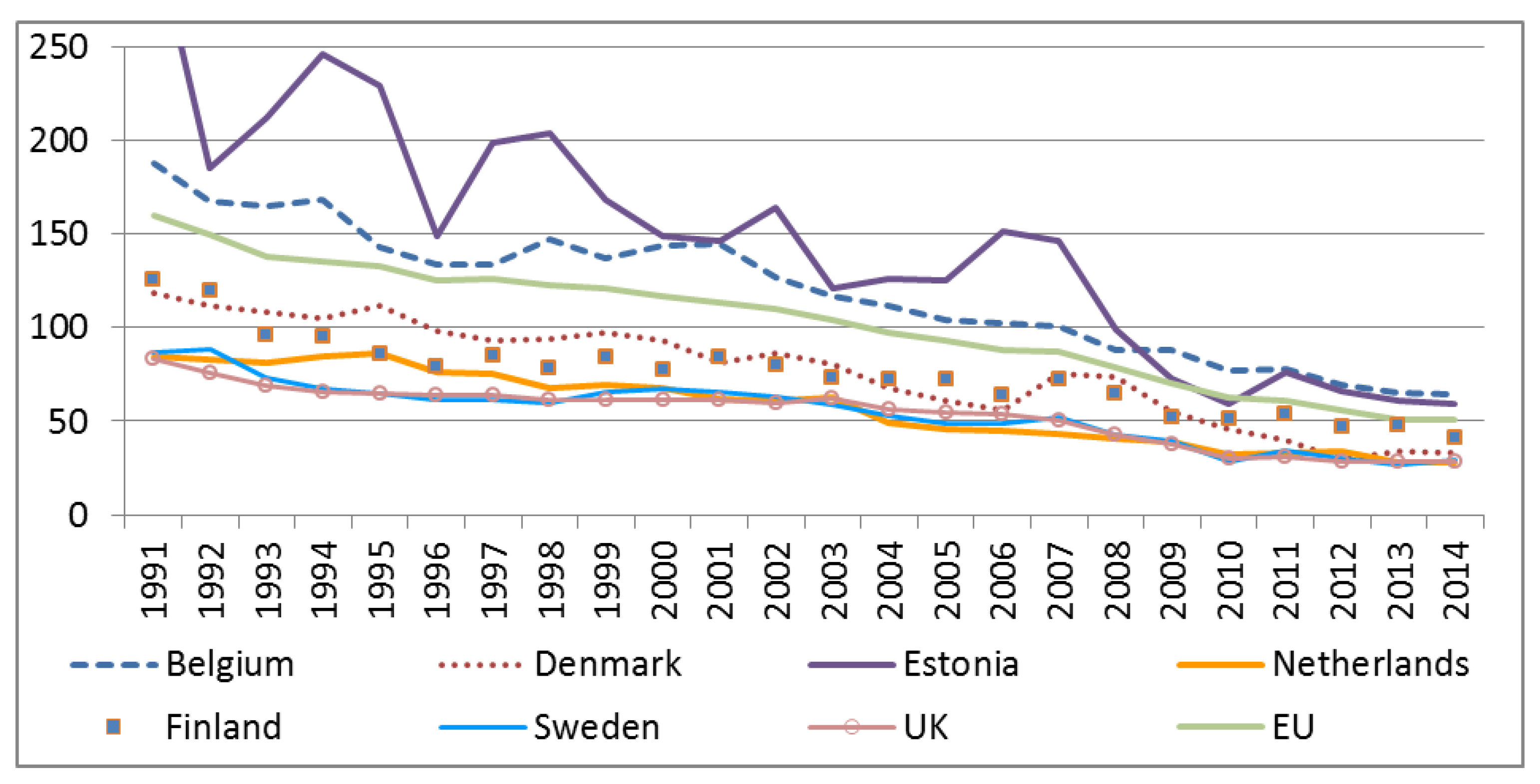
As in many European countries, road safety in Finland has steadily improved over the past decades (Figure 1). Unusually harsh winters with more than average crashes, or winters in which a few crashes with a large number of fatalities occurred, are reasons for deviations from the trend in some years.

Figure 1. Number of fatalities per million inhabitants. Source: EC DG Mobility and Transport—Road Safety Statistics website [30].

Figure 1. Number of fatalities per million inhabitants. Source: EC DG Mobility and Transport—Road Safety Statistics website [30].

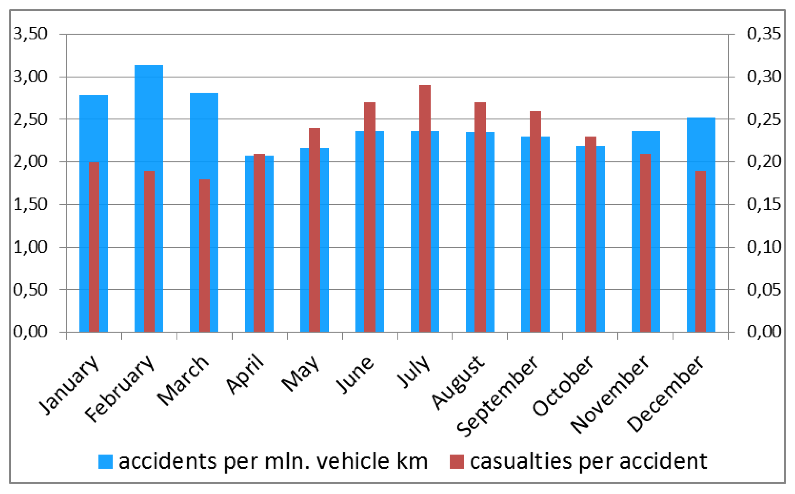
It is important to realise that the number of crashes and the number of casualties are not completely proportional to each other (Figure 2). Average speeds on main roads and highways are lower in winter due to decreased visibility and increased slipperiness, whereas the average number of passengers per car tends to be higher in summer [31]. The combined effect is that the crash rate and indeed also average daily number of crashes is the highest in winter months, but the daily number of casualties is the highest in summer months. Traffic volumes are a bit higher outside the summer months. This volume effect only adds to the effect of higher crash rates, resulting in higher absolute numbers of crashes outside the summer months. 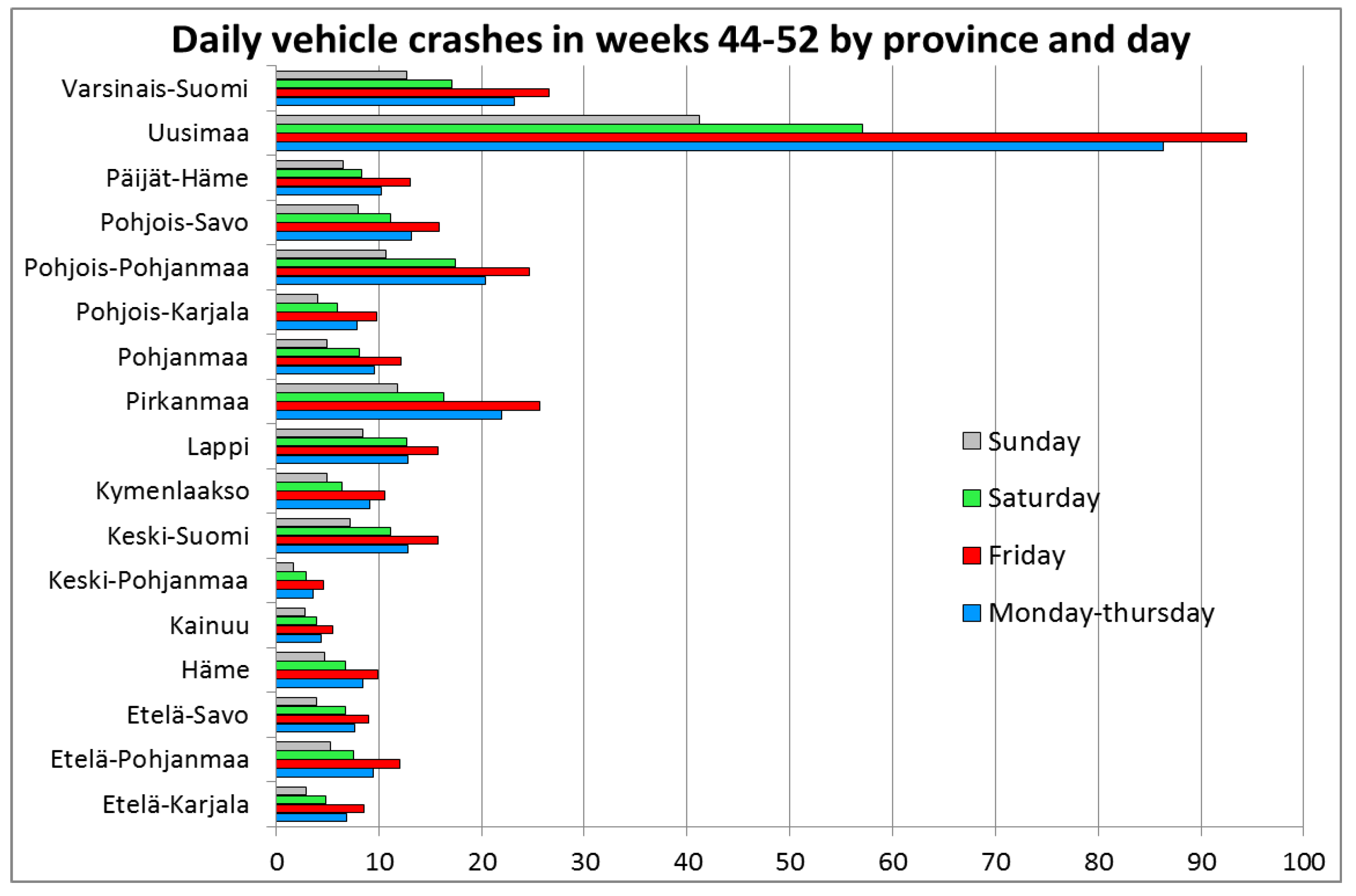Apart from the seasonal effect, days of the week have different risk profiles (Figure 3). Firstly, busier traffic on working days raises the crash risk as compared to quieter weekend days. Secondly, Fridays stand out as the riskiest. These differences relate to differences in typical daily activity patterns and space-time profiles.

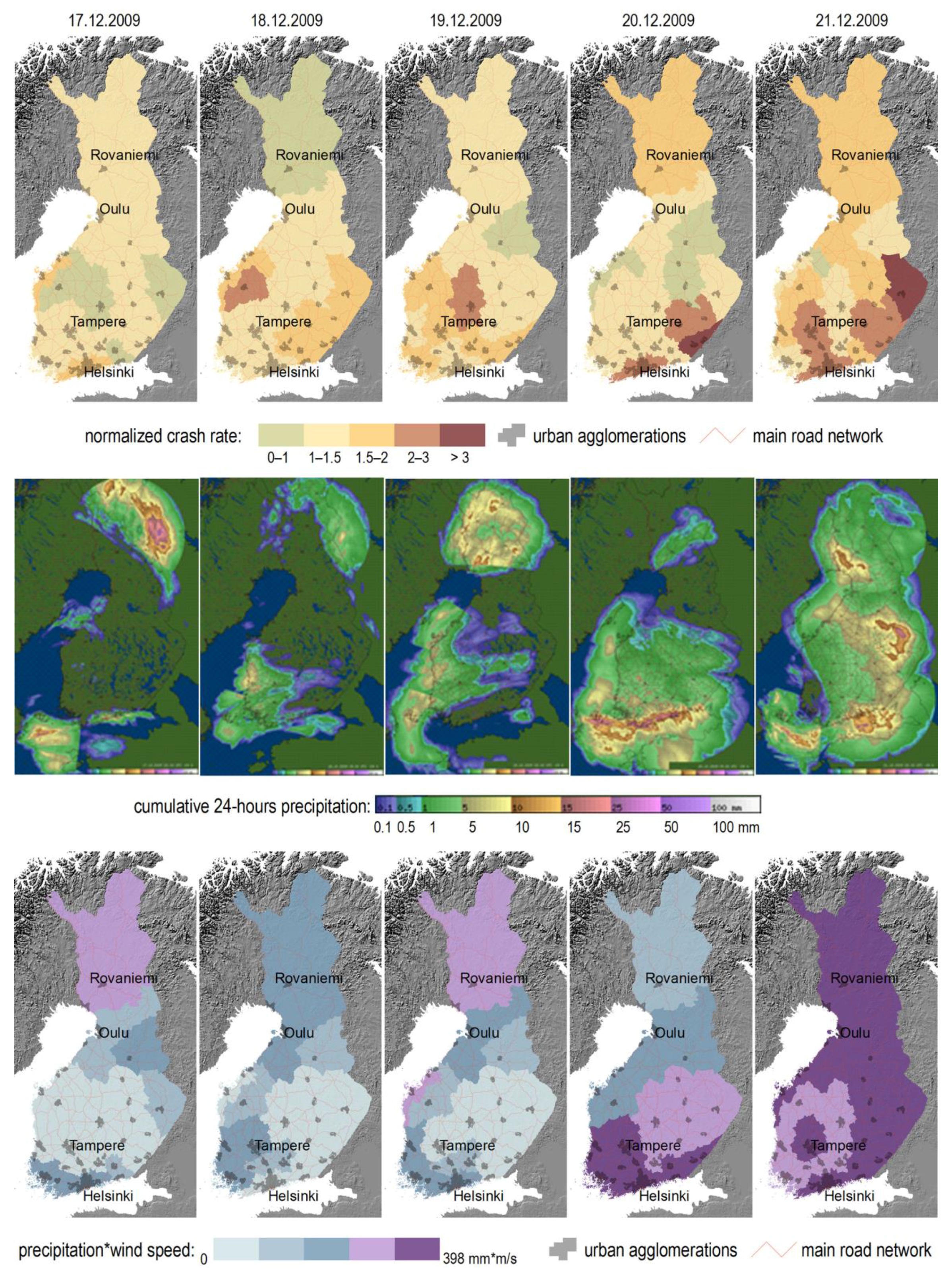
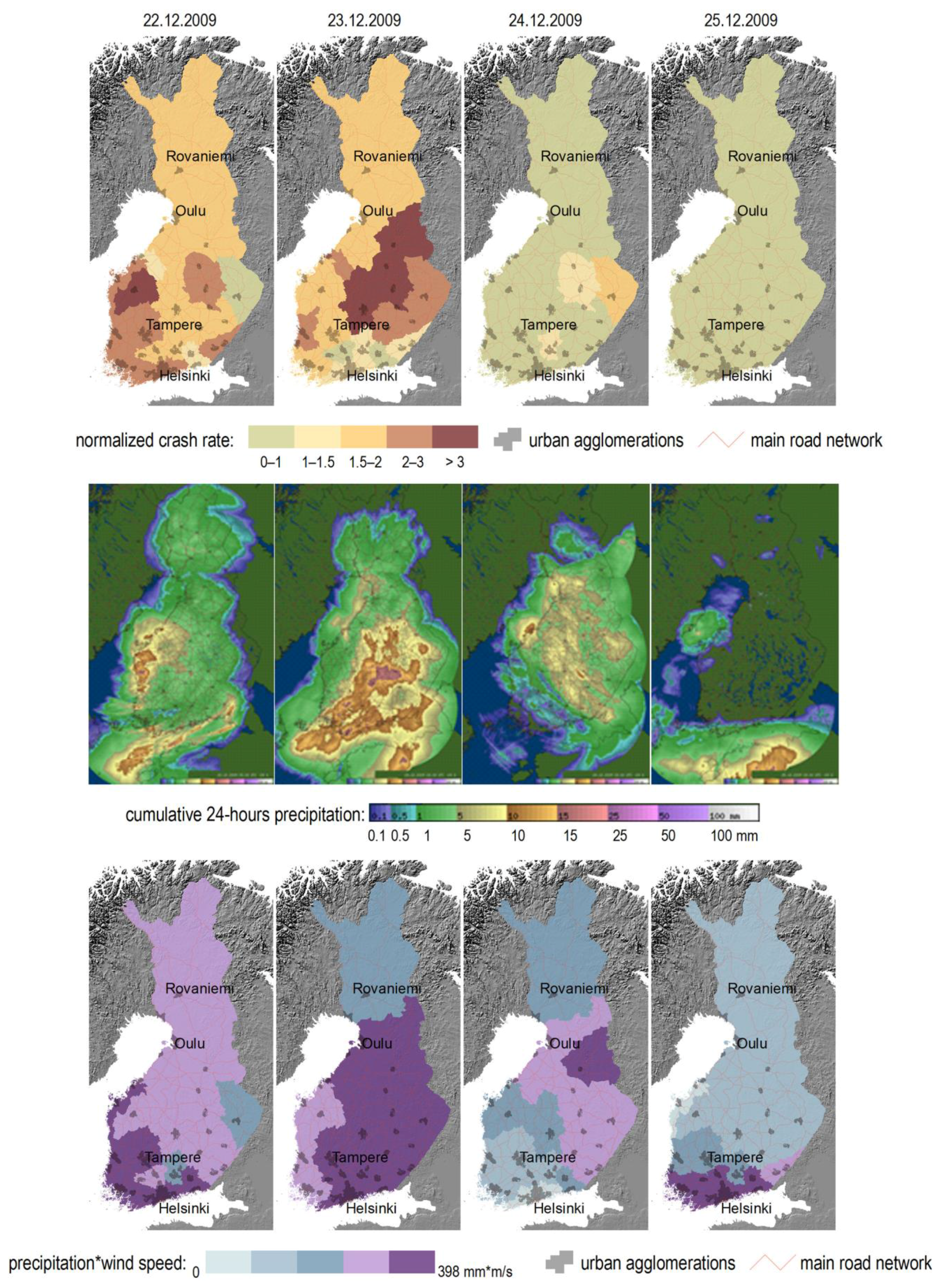
Spatially defined differences in the crash risk are, among others, related to traffic intensity, due to for instance higher population density in certain areas, but also to spatially defined differences, which often relate to weather conditions. Variations in the physical geography of regions often translate into structural differences in crash-relevant weather patterns. For instance, coastal provinces are subject to higher average and higher maximum wind speeds than inland regions (except for the hill tops in Lapland, but there is no traffic). The best way to illustrate this connection is to consider crash rates in different regions in relation to severe weather trajectories. Over the course of an unfolding storm trajectory during a day, detrimental conditions for traffic will not appear in the same location at the same time, or even do not appear at all in many regions located in the storm trajectory. Figure 4 illustrates this spatial variation for an extensive storm event over Finland during a nine-day period in December 2009. The first (upper) set of maps displays the daily crash rate per NUTS-3 region, normalized by the baseline average daily crash rate for the period November–December. The second (middle) set displays radar derivatives of the cumulative precipitation volume for each day. The third (lower) set displays the product of average wind speed and precipitation per day and region.

Figure 2. Monthly crash rates (crashes per million vehicle km) and average number of casualties per accident for the period 2000–2010. (crash rates: left-hand scale; casualties: right-hand scale). Source: study dataset (see Section 3).

Figure 2. Monthly crash rates (crashes per million vehicle km) and average number of casualties per accident for the period 2000–2010. (crash rates: left-hand scale; casualties: right-hand scale). Source: study dataset (see Section 3).

Figure 3. Daily number of crashes by day of the week by region in November and December 2000–2010. Source: study dataset (see Section 3).

Figure 3. Daily number of crashes by day of the week by region in November and December 2000–2010. Source: study dataset (see Section 3).

Figure 4. An example of spatiotemporal association between crash rates and severe weather.

Figure 4. An example of spatiotemporal association between crash rates and severe weather.

The radar images show that as the storm progressed over Finland, the heaviest accumulated precipitation is concentrated over specific regions in a given day, and this corresponds with peaks in the normalized crash rates of those regions in those days; see for instance the maps of 20, 21, 22, and 23 December. While radar maps are good for providing evidence regarding coincidence of storms and accident rates and regional differences therein, the statistical model in Section 5 shows that a combination of weather parameters is a better predictor of road accidents. This is echoed in Figure 4 (bottom row) with combined wind speed and precipitation; see for instance 20 and 22 December.

Overall, Figure 4 indicates an apparent sequential spatial clustering of crash frequencies, implying that similar (diurnal variation of) accident rates occur in daily clusters of adjacent regions. Severe weather trajectories constitute a natural candidate for the underlying process generating this sequential clustering, as similar weather conditions often will affect large expanses of adjacent regions during consecutive days. However, formal statistical analysis is necessary for verifying this assumption, for identifying additional spatial processes, and for formally testing and modelling the space-time clusters of accident rates, weather, and other factors in a multivariate setting.

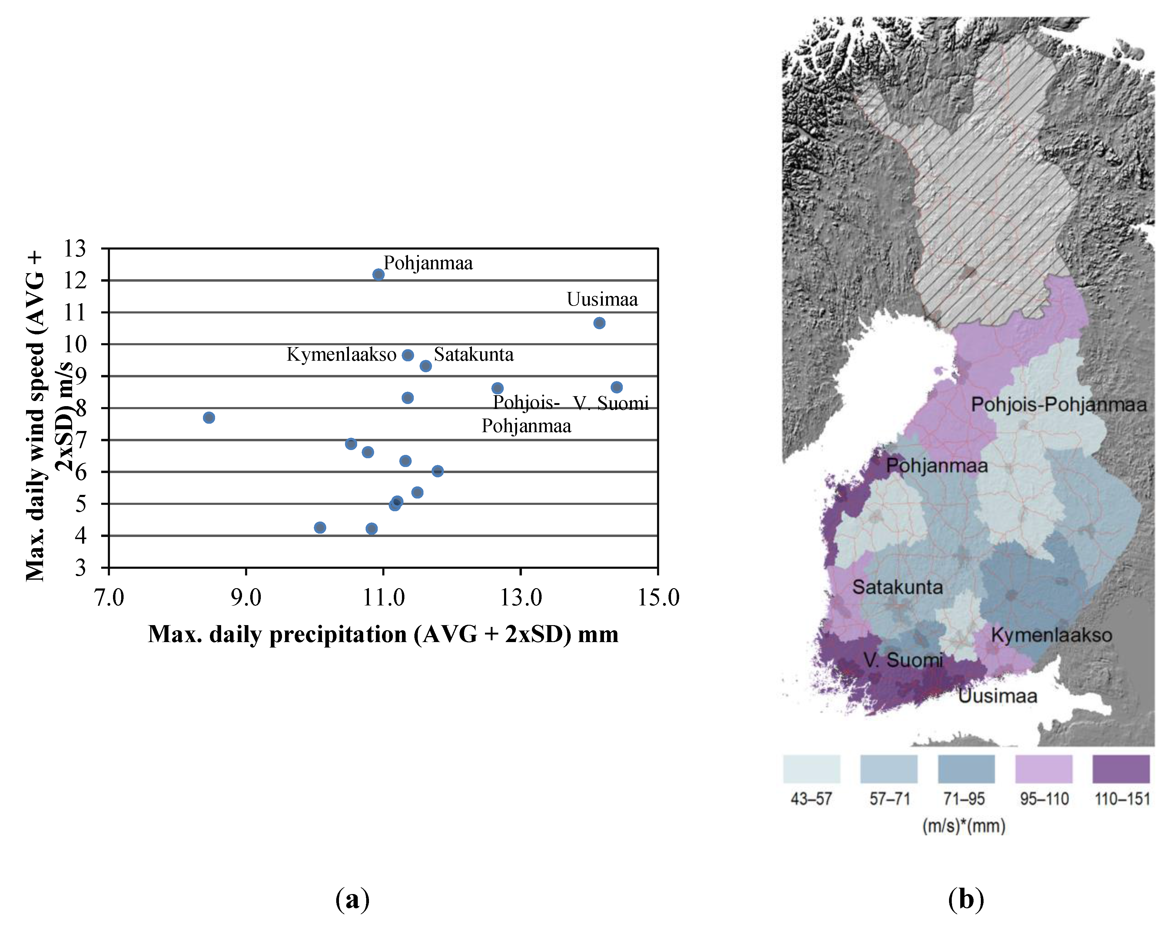
Figure 5. (a) Scatterplot of daily averages augmented by 2x standard deviation for precipitation and wind speed by region in winter periods based on observations from 2000 to 2010; and (b) Regional clustering (along the coast) of the highest observed combined wind speed and precipitation maximums (product of both values).

Figure 5. (a) Scatterplot of daily averages augmented by 2x standard deviation for precipitation and wind speed by region in winter periods based on observations from 2000 to 2010; and (b) Regional clustering (along the coast) of the highest observed combined wind speed and precipitation maximums (product of both values).

Apart from illustrating the spatial co-occurrence of bad weather and increases in car crashes, weather patterns have also spatial distributions which are relevant for the distribution of accident proneness across the country. This is illustrated by means of the structural co-occurrence of strong winds and intensive precipitation (in winter in this case) (Figure 5). When wind speed and precipitation jointly increase in strength, not only grip of tires, but especially visibility, deteriorates. Coastal areas are exposed to higher average and maximum wind speeds than inland areas. However, the intensity of heavy snowfall has a less pronounced spatial distribution (even though climate change may intensify extreme snowfall hazards along the Finnish south coast [32]). The spatial wind speed gradient seems to be stronger and clearer than the intense snowfall gradient, while it partly coincides with it. This implies that coastal areas are supposedly more prone to adverse weather induced car crash risks. As it happens, several of these areas are also more densely populated than an average Finnish region.

5. A Model of Road Vehicle Crash Rate Sensitivity to Adverse Weather Conditions

The car crash model presented in this section is as yet explorative and is developed to obtain a better understanding of the influence of various weather parameters on the probability of accidents at aggregate levels; for a given network flow per day. It was not specifically developed for crisis management support. The model does not reflect physical causal processes leading to a crash. Instead, it provides an indication of the number of surplus crashes per region in relation to changes in weather conditions relevant for road traffic. The presented estimations results concern the Finnish road network. The same model—with re-estimated parameter values—could perform also satisfactorily in Sweden and Norway due to similar climatology and level of preparedness for winter weather. For other countries, larger modifications in the model may be necessary.

The model deals with winter road weather circumstances, as this is the period of the year during which vehicle drivers are facing much more frequently and to some extent practically permanently weather hazards. Snowfall, snow cover, icing, winter storms, and lack of daylight imply that both slipperiness and hampered visibility are recurrent safety hazards. This backdrop explains the choice of the variables. In case there were closely related variables available, e.g., maximum daily temperature or average daily temperature, the best performing variety was retained. Fog is not included, as it is rather seldom a significant road traffic hazard in Finland (i.e., fog is seldom truly dense); moreover, it is often a localized phenomenon and therefore is not always well captured by the observation system.

5.1 Model Implementation

Due to the variation in the size of the regions and car fleet, and different degrees of transit functions in inter-regional transport, crash rate is used as the independent variable instead of the absolute number of crashes. It enables easier comparison between days of the week and seasons with respect to other risk factors than traffic volume. The effect of traffic volume on the total number of crashes per day can eventually be added (by region, season, etc.).

Considering the lack of variables regarding the state of the driver and the vehicle, and considering the matching of crashes and weather at the level of a whole day (instead of hourly or by part of the day), more complex structures (e.g. nested or conditional) seemed of little use. Similarly, the lack of observations of bad weather days without warnings precluded use of a Difference in Differences approach. As observations do not concern a particular road stretch, and neither have an hourly or nearly hourly resolution, Poisson regression was no option either. The Ordinary Least Squares method seemed the best step at this stage, also because we are interested in getting an idea of the distinct contribution of each weather variable, rather than comparing weather condition classes. It was regarded of more importance to exploit the available variables as well as possible, and to consider the relevance of interaction effects, such as for wind and precipitation. Moreover, segmentation in sub-seasons and typical days of the week, which in fact captures some of the variation in variables not observed in the equations, improves the quality of the equations. For example, the different weekdays represent differences in traffic patterns, and tightness of daily schedules. Moreover, the addition of quadratic forms of variables was tested, but none were significant.

The general specification of the estimated function is:

$$\ln \left(A_{dsr}\right)={\alpha }_{dsr}+{\displaystyle \sum }_i{\beta }_{idsr}·\ln \left(W_{idsr}\right)+{\gamma }_{jdsr}·D_{jdsr}+{\displaystyle \sum }_l{\theta }_{ldsr}·\ln \left(T_{ldsr}\right)$$

(1)

where A_dsr denotes the crash rate (number of crashes per million vehicle kilometres) in the considered area r (region or combination of regions) in season s (November–December or January–March) and on type of day d (Monday–Thursday, Friday, Saturday, Sunday).

W_idsr denotes a vector of explanatory weather related variables i = 1 to 6, being: (1) average temperature (Celsius), (2) maximum precipitation within the area (mm), (3) average wind speed (meters/second), (4) maximum relative humidity (percentage points 0–100), (5) snow depth (centimetres), (6) average precipitation x wind speed (interaction variable). All these variables refer to daily observations (possibly averaged over space). For below zero temperatures, the natural logarithm is applied to −1. T_ave, while the result is multiplied by −1.

D_jdsr denote dummy variables related to weather circumstances characterized by distinct states, such as freezing or not freezing (D = 1 if in state “A” and D = 0 if not in state “A”). In the results presented in Section 5.2, only the dummy for the occurrence per day of the freeze-thaw cycle is included, in which case “D = 1” represents a freezing state and “D = 0” a non-freezing state.

T_ldsr denote transport system related variables, numbered l = 1 to 2, being (1) traffic intensity on main roads (weighted average number of vehicles passed by road segment) and (2) the percentage share of motorways in a region’s road network (traffic weighted, expressed in percent points).

α, β, γ, and θ are the respective regression coefficients. The estimated values of the regression coefficients are presented in Section 5.2.

Dummy variables for the occurrence of bad driving weather warnings were also explored. The conditional validity of these warnings seems to be more complex, whereas comparable cases with equally bad weather with and without warnings, respectively, (and otherwise comparable circumstances) are extremely scarce. At this stage, it was decided not to include the warning dummy variables.

5.2 Results and Discussion

Table 2 and Table 3 present the estimated values of the regression coefficients for eight different regressions (1) Monday to Thursday in November and December; (2) Monday to Thursday in January to March; (3) Fridays in November and December; (4) Fridays in January to March; (5) Saturdays in November and December; (6) Saturdays in January to March; (7) Sundays in November and December; (8) Sundays in January to March, the standard error of the estimates and the Student test value (t-statistic) indicating the statistical significance of a variable. For example, in Table 2 concerning working days (Monday–Thursday), the variable ln_RRmax (maximum precipitation on a day) is not significant in early winter (November–December), whereas it is significant later on in winter (January–March).

Table 2 and Table 3 can be used to apply the above presented specification form as follows (example for November–December/Monday–Thursday):

$$\begin{array}{l}\ln (A_{dsr})=0.85216+0.03511\ln (T_{ave})+0.03011\ln (W_{savg})-\\ 0.62942\ln (R{h}_{\max })+0.07360\ln (snowdp)+0.05606\ln (prepxwind)+\\ 0.40566\ln (tcarsperday)-0.11191\ln (pchighways)+0.11245D_{Thaw}\end{array}$$

(2)

The coefficients of determination (R²) vary between 0.08 for early winter Sundays to 0.19 for early winter working days (Monday–Thursday). This moderate—yet significant—explanatory power of the estimations indicates that weather circumstances are generally not a dominant source of collisions, even in winter. More precise traffic flow data and more elaborate treatment of the warnings probably would lift the explanatory power to some extent.

The estimations have been made separately for the first four working days (Monday–Thursday), Fridays, Saturdays, and Sundays because the typical trip composition of road traffic varies significantly between these different groups of days. In addition, average traffic performance differs for these days. This affects the degree of haste, distribution of driving skills of involved drivers, and ability to avoid bad weather by postponing the trip or switching mode. This shows in the statistics as significantly different average accident intensities for these different days. Moreover, early winter and late winter are distinguished due to different crash rates in these periods. These differences are probably caused by attitudinal changes in winter preparedness and driving skill evolvement during winter time [33], but we did not find further literature on hard evidence for the causes of these differences.

Maximum daily precipitation within the area (RRmax) appears to be statistically significant only during working days (Monday–Thursday) in January–March and, in fact, a border case in statistical significance on Fridays during November–December. Since effects of precipitation are also captured by the compound variable PREPxWIND, the results seem to indicate that more intense precipitation in the form of rain (which is still the more prevailing form for the greater part of November–December, while never as intense as summer downpours) is not easily raising crash rates, if wind speeds remain moderate. On the other hand, the lack of statistical significance for weekend days could be explained by the increased willingness to postpone trips and to reduce speeds as time pressures tend to be lower than on weekdays. Friday is probably the day with the highest average time pressures, which would reduce the willingness to postpone trips when heavy precipitation is projected.

Table 2. Regression estimations for Monday–Thursday and Friday for all regions together.

Dependent Variable: Crash Rate	Monday–Thursday November–December			Monday–Thursday January–March			Friday November–December			Friday January–March
Explanatory Variables:	Coefficient	Standard Error	t Statistic	Coefficient	Standard Error	t Statistic	Coefficient	Standard Error	t Statistic	Coefficient	Standard Error	t Statistic
Intercept	0.85216	0.8685	0.98	−5.41001	0.4874	−11.10	0.37749	1.3623	0.28	−2.76251	0.9712	−2.84
Widsr:
ln_Tave	0.03511	0.0081	4.34	0.10520	0.0063	16.65	0.04802	0.0162	2.97	0.05707	0.0130	4.40
ln_RRmax	0.01244	0.0133	0.93	0.02594	0.0116	2.23	0.04863	0.0258	1.89	0.01151	0.0241	0.48
ln_Wsavg	0.03011	0.0106	2.83	0.06744	0.0082	8.22	0.05482	0.0193	2.84	0.06177	0.0156	3.95
ln_Rhmax	−0.62942	0.1882	−3.35	0.76484	0.1060	7.22	−0.30317	0.2948	−1.03	0.28797	0.2105	1.37
ln_snowdp	0.07360	0.0042	17.45	0.08694	0.0055	15.75	0.01530	0.0084	1.82	0.11470	0.0107	10.72
ln_prepxwind	0.05606	0.0102	5.48	0.05949	0.0090	6.58	0.00696	0.0195	0.36	0.08894	0.0187	4.76
Tldsr:
ln_tcarsperday	0.40566	0.0123	33.08	0.37779	0.0103	36.70	0.26676	0.0241	11.08	0.33361	0.0204	16.32
ln_pchighways	−0.11191	0.0221	−5.06	−0.11448	0.0177	−6.46	−0.01859	0.0432	−0.43	−0.10225	0.0356	−2.88
Djdsr:
D_Thaw	0.11245	0.0171	6.59	0.01607	0.0136	1.18	0.08029	0.0339	2.37	−0.06639	0.0282	−2.35
N	6942			9657			1698			2450
R2	0.192			0.184			0.104			0.168

Table 2. Regression estimations for Monday–Thursday and Friday for all regions together.

Dependent Variable: Crash Rate	Monday–Thursday November–December			Monday–Thursday January–March			Friday November–December			Friday January–March
Explanatory Variables:	Coefficient	Standard Error	t Statistic	Coefficient	Standard Error	t Statistic	Coefficient	Standard Error	t Statistic	Coefficient	Standard Error	t Statistic
Intercept	0.85216	0.8685	0.98	−5.41001	0.4874	−11.10	0.37749	1.3623	0.28	−2.76251	0.9712	−2.84
Widsr:
ln_Tave	0.03511	0.0081	4.34	0.10520	0.0063	16.65	0.04802	0.0162	2.97	0.05707	0.0130	4.40
ln_RRmax	0.01244	0.0133	0.93	0.02594	0.0116	2.23	0.04863	0.0258	1.89	0.01151	0.0241	0.48
ln_Wsavg	0.03011	0.0106	2.83	0.06744	0.0082	8.22	0.05482	0.0193	2.84	0.06177	0.0156	3.95
ln_Rhmax	−0.62942	0.1882	−3.35	0.76484	0.1060	7.22	−0.30317	0.2948	−1.03	0.28797	0.2105	1.37
ln_snowdp	0.07360	0.0042	17.45	0.08694	0.0055	15.75	0.01530	0.0084	1.82	0.11470	0.0107	10.72
ln_prepxwind	0.05606	0.0102	5.48	0.05949	0.0090	6.58	0.00696	0.0195	0.36	0.08894	0.0187	4.76
Tldsr:
ln_tcarsperday	0.40566	0.0123	33.08	0.37779	0.0103	36.70	0.26676	0.0241	11.08	0.33361	0.0204	16.32
ln_pchighways	−0.11191	0.0221	−5.06	−0.11448	0.0177	−6.46	−0.01859	0.0432	−0.43	−0.10225	0.0356	−2.88
Djdsr:
D_Thaw	0.11245	0.0171	6.59	0.01607	0.0136	1.18	0.08029	0.0339	2.37	−0.06639	0.0282	−2.35
N	6942			9657			1698			2450
R2	0.192			0.184			0.104			0.168

Table 3. Regression estimations for Saturday and Sunday for all regions together.

Dependent Variable: Crash Rate	Saturday November–December			Saturday January–March			Sunday November–December			Sunday January–March
Explanatory Variables:	Coefficient	Standard Error	t Statistic	Coefficient	Standard Error	t Statistic	Coefficient	Standard Error	t Statistic	Coefficient	Standard Error	t Statistic
Intercept	2.21916	1.5590	1.42	−2.71915	0.9143	−2.97	3.96220	1.8090	2.19	−7.00080	1.1439	−6.12
Widsr:
ln_Tave	0.01206	0.0163	0.74	0.08378	0.0123	6.83	0.02598	0.0182	1.43	0.09357	0.0143	6.54
ln_RRmax	−0.01129	0.0289	−0.39	0.02260	0.0225	1.00	0.04694	0.0294	1.60	0.04009	0.0263	1.53
ln_Wsavg	−0.00563	0.0222	−0.25	0.10774	0.0167	6.46	0.02114	0.0242	0.87	0.06690	0.0190	3.52
ln_Rhmax	−0.83380	0.3363	−2.48	0.37713	0.1989	1.90	−1.29335	0.3900	−3.32	1.19153	0.2498	4.77
ln_snowdp	0.05299	0.0092	5.77	0.08812	0.0105	8.38	0.06043	0.0098	6.15	0.06607	0.0123	5.39
ln_prepxwind	0.04281	0.0220	1.94	0.05412	0.0178	3.05	−0.01074	0.0229	−0.47	0.02365	0.0198	1.19
Tldsr:
ln_tcarsperday	0.29203	0.0263	11.12	0.20971	0.0207	10.14	0.31532	0.0278	11.33	0.23327	0.0240	9.73
ln_pchighways	−0.01010	0.0469	−0.22	−0.09658	0.0358	−2.70	−0.05759	0.0496	−1.16	−0.04948	0.0412	−1.20
Djdsr:
D_Thaw	0.13078	0.0352	3.71	−0.03595	0.0289	−1.25	0.07345	0.0391	1.88	−0.00600	0.0314	−0.19
N	1644			2476			1607			2449
R2	0.102			0.127			0.082			0.100

Table 3. Regression estimations for Saturday and Sunday for all regions together.

Dependent Variable: Crash Rate	Saturday November–December			Saturday January–March			Sunday November–December			Sunday January–March
Explanatory Variables:	Coefficient	Standard Error	t Statistic	Coefficient	Standard Error	t Statistic	Coefficient	Standard Error	t Statistic	Coefficient	Standard Error	t Statistic
Intercept	2.21916	1.5590	1.42	−2.71915	0.9143	−2.97	3.96220	1.8090	2.19	−7.00080	1.1439	−6.12
Widsr:
ln_Tave	0.01206	0.0163	0.74	0.08378	0.0123	6.83	0.02598	0.0182	1.43	0.09357	0.0143	6.54
ln_RRmax	−0.01129	0.0289	−0.39	0.02260	0.0225	1.00	0.04694	0.0294	1.60	0.04009	0.0263	1.53
ln_Wsavg	−0.00563	0.0222	−0.25	0.10774	0.0167	6.46	0.02114	0.0242	0.87	0.06690	0.0190	3.52
ln_Rhmax	−0.83380	0.3363	−2.48	0.37713	0.1989	1.90	−1.29335	0.3900	−3.32	1.19153	0.2498	4.77
ln_snowdp	0.05299	0.0092	5.77	0.08812	0.0105	8.38	0.06043	0.0098	6.15	0.06607	0.0123	5.39
ln_prepxwind	0.04281	0.0220	1.94	0.05412	0.0178	3.05	−0.01074	0.0229	−0.47	0.02365	0.0198	1.19
Tldsr:
ln_tcarsperday	0.29203	0.0263	11.12	0.20971	0.0207	10.14	0.31532	0.0278	11.33	0.23327	0.0240	9.73
ln_pchighways	−0.01010	0.0469	−0.22	−0.09658	0.0358	−2.70	−0.05759	0.0496	−1.16	−0.04948	0.0412	−1.20
Djdsr:
D_Thaw	0.13078	0.0352	3.71	−0.03595	0.0289	−1.25	0.07345	0.0391	1.88	−0.00600	0.0314	−0.19
N	1644			2476			1607			2449
R2	0.102			0.127			0.082			0.100

Average temperature and wind speed on the other hand are significant in most cases, and the estimated parameters are systematically larger in the late winter period as compared to the early winter period, meaning that there is more impact per incremental unit of wind or temperature. Snow depth is statistically significant in most cases. The variable is expected to function as a proxy variable for degree of road clearance. With increasing snow depth, probability that secondary roads are not entirely clear anymore increases. Wind can also disperse subsided snow back on the road.

Noticeable is also that the freeze-thaw cycle tends to increase crash rates in early winter, whereas it tends to reduce them in late winter (or is not statistically significant). It is unclear to what extent this has to do with learning, late switching to winter tires, differences in the amount of daylight or with physical differences in freeze-thaw cycles in these two periods. The effect of the share of highways in the regional road system is higher during working days than on Fridays and weekend days, which probably reflects other routing patterns on those days.

Nurmi et al. [2] estimated the effect of weather information on the occurrence of weather related crashes at a 14% reduction as annual average (in terms of avoided crashes). This 14% reduction refers to all road weather information together, not only warnings. As mentioned earlier, Cools et al. [26] showed that adverse weather tends to reduce traffic volume (roughly by −3% to −7% in the case of Belgium). As the model presented here is based on realized accidents, the estimated (and observed) increase in accident rates includes the just mentioned response effects. Considering simulation outcomes concerning effects of weather informedness on trip generation and mode choice [34,35] we may assume that the estimated propensity of response to weather features (wind speed, etc.) is not significantly affected by this traffic reduction effect, but we admit that may be also skill related selectivity involved in the traffic reduction effect. This means that the original—unmitigated or non-anticipated—hazard effect of bad weather in absolute numbers is roughly 15% to 20% larger than the estimated effects (absence of a warning effect means 14/86 ~ 16.3% and absence of traffic reduction would add some other percentage points—even though there will be anyhow some last minute traffic reduction regardless of warnings).

5.3 Examples of Use of the Model

By inserting average values for the explanatory variables for winter time (per part-season and type of day) or values for a “nice winter day”, one obtains an estimate for the average crash intensity for such a typical day. Subsequently, values for bad and very bad weather can be inserted in order to assess to which intensity level the accident rate rises. The difference in intensity levels is an indication of the effect of bad weather. Table 4 provides an example for input values reflecting three winter weather situations for the country as a whole. Especially for the case of very bad weather, it may mean that the number of crashes rises to about 325 instead of 336. The expected number of crashes related to bad weather can be rated at 46 (surplus crashes on one day) for bad weather and 65 (surplus crashes on one day) for very bad weather for the current level of average traffic volumes.

Table 4. Illustration of effects of different levels of input variables reflecting different weather conditions.

Input Values	Normal	Bad	Very Bad
Wsavg average wind speed (m/s)	3	13	17
Tave average temperature (°C)	–3	–7	–7
RRmax maximum precipitation (mm/day)	5	15	25
Rhmax maximum humidity	97	97	97
Thaw occurrence of freeze-thaw cycle	1	1	1
Snowdp snow depth (cm)	22	42	42
Prepxwind (RRmax x Wsavg)	15	105	221
Tcarsperday traffic intensity	1020	1020	1020
Pchighways % share of highways in traffic performance	13	13	13
Resulting crash rate (N/million vkm)	2.7374	3.2043	3.3894
N crashes (on one day)	271	317	336

Table 4. Illustration of effects of different levels of input variables reflecting different weather conditions.

Input Values	Normal	Bad	Very Bad
Wsavg average wind speed (m/s)	3	13	17
Tave average temperature (°C)	–3	–7	–7
RRmax maximum precipitation (mm/day)	5	15	25
Rhmax maximum humidity	97	97	97
Thaw occurrence of freeze-thaw cycle	1	1	1
Snowdp snow depth (cm)	22	42	42
Prepxwind (RRmax x Wsavg)	15	105	221
Tcarsperday traffic intensity	1020	1020	1020
Pchighways % share of highways in traffic performance	13	13	13
Resulting crash rate (N/million vkm)	2.7374	3.2043	3.3894
N crashes (on one day)	271	317	336

Figure 6. (a) Road vehicle crash rates (per million vehicle kilometers) in normal weather conditions in 2000 per Finnish province; (b) Crash rates in normal weather conditions in 2010, and growth from 2000; (c) Crash rates in very bad weather conditions in 2010. The colour scale divisions are common for all maps.

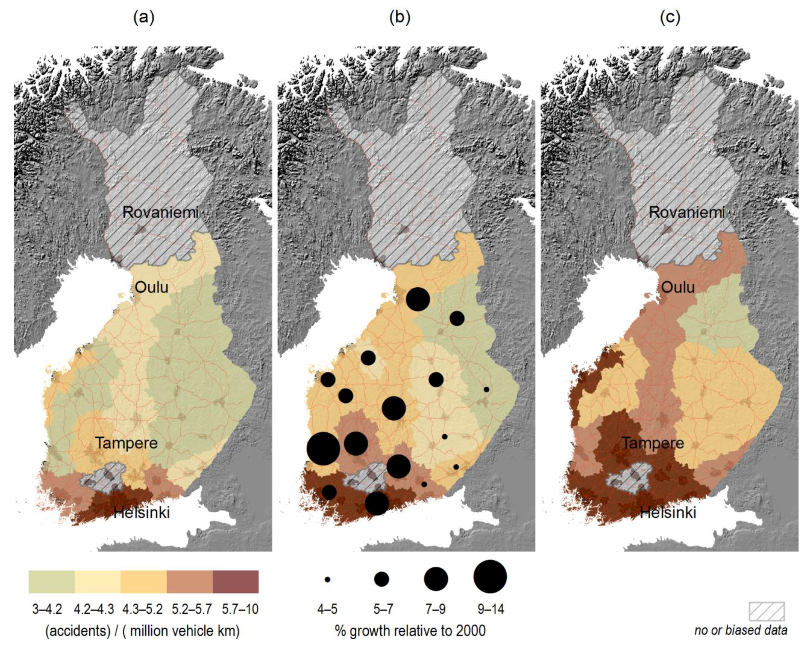
Figure 6. (a) Road vehicle crash rates (per million vehicle kilometers) in normal weather conditions in 2000 per Finnish province; (b) Crash rates in normal weather conditions in 2010, and growth from 2000; (c) Crash rates in very bad weather conditions in 2010. The colour scale divisions are common for all maps.

The above example can be regionalized by replacing the national averages with the specific values that the variables of Table 4 take in each Finnish region for normal, bad, or very bad weather conditions shown in Figure 6. Figure 6a,b display the change in crash rates during normal winter weather conditions from between 2000 and 2010, with the growth in these crash rates ranging from 4% in the Eastern regions to 14% in the Western region of Satakunta. These differences in growth (between Figure 6a and 6b) have mainly to do with differences in the development of regional traffic volumes. The capital region of Uusimaa exhibits the highest crash rate but not the highest growth. Figure 6c displays the crash rate in 2010 during (hypothetical) very bad winter weather conditions. The regional distribution of these elevated rates is loosely echoing that of combined extreme wind-speed and precipitation in Figure 5b. The difference is that due to strong traffic volume growth in the 2010 baseline, a few inland provinces are lifted into the same category in which most coastal provinces are.

6. Discussion

Geographically referenced information is helpful for quick identification and communication of localized accident risks, which, in turn, can support preparedness planning and optimal deployment of rescue and health services at regional levels. Georeferenced data can also enhance in-depth quantitative analysis, as most appropriate spatial and temporal resolutions for the estimation input data and for segmentations in the analysis can be identified. However, this highly supportive role should not be confused with inference of existence of highly significant spatial causation. Some truly spatial causation factors exist, such as variation of geophysical characteristics in space, causing systematic differences in the distributions of weather variables. The dominant influence factors of crash rates (e.g., the condition and skills of the driver) do not, however, seem to entail spatial mechanisms at higher spatial aggregation levels, even though there may appear spatial clustering in their occurrence. This notion ties in with the problem that residence linked characteristics get dissolved when drivers disperse over a larger space.

As indicated above, only some factors, out of the large portfolio of factors affecting crash rates, involve genuine spatial differentiation mechanisms. In the analysis, we identified nearness to the coast as a spatial factor playing out through systematic weather variable differences. Furthermore, in the discussion, landscape and residential neighbourhood peer processes regarding driving style and car choice were put forward. Owing to the lack of personal data, the latter type of influence could not be assessed. Yet, the available literature suggests that the effects may be only relevant for certain groups.

As regards estimation quality, higher spatial and temporal resolution data could still improve the accuracy of the estimations, even though very high resolutions are probably not productive due to stochastic elements in the spatial occurrence of weather extremes and crashes. The projections based on these higher resolutions could benefit also from continuous traffic monitoring systems (with implicit high resolutions) to enhance the relevance for deployment of rescue and health services. Another issue regarding estimation quality constitute the various truncation and censoring effects. The partial exclusion of some sorts of accidents and the deterrence effects of weather information and bad weather merit additional analysis with respect to possible corrections in estimated weather sensitivities. These corrections may also have effects on estimated net societal benefits of road weather information services.

7. Conclusions

According to the estimation results, on some days, bad weather can raise the number of accidents significantly (by 20% or more over the base rate). We have not assessed whether bad winter weather affects casualty numbers to the same extent. The literature suggests that there may be a somewhat attenuated effect on casualty numbers thanks to speed reductions, but this may not be true for all adverse weather situations.

Wind speed, precipitation intensity and temperature all appear to be significant in most cases. The combination of wind speed and precipitation especially matters. The sensitivity to bad weather appears to vary over the different days. The more cramped daily schedules tend to be the less willingness there is to adapt travel schedules, despite (forecast) bad weather. Therefore, weekend traffic seems to be less sensitive to bad weather than working day traffic, in particular Fridays. Freezing and thawing on the same day adds notably to crash risks in the early winter months (November–December), but not anymore later on in the winter. For other weather variables coefficients are larger (i.e., sensitivity is stronger) in the period January–March. Nevertheless, traffic volume appears to be the most significant variable at this level of analysis (daily average traffic density), but obviously will not explain the weather related peaks in crash occurrences.

Climate change is expected to increase strong winds and intense snowfall to some extent in the coming decades [32]. Even if we assume that both the frequency and maxima increase by 10%, the number of surplus crashes per year does not rise enormously, being somewhere between 10 and 40. As can be inferred from Figure 3 and Table 3, the climate change effect is very modest given the total number of crashes per day. Yet, apart from the uncertainties regarding how strongly climate change may affect storminess and extreme precipitation, climate change may also cause rises in other hazardous road conditions, which have not yet been identified.

This study focused in particular on winter weather risks for road traffic, but the higher casualty rates in summer merit attention just as well. Furthermore, with expected hotter summers and more extreme summer downpours, crash rates may rise as a consequence of climate change. Climate change is also expected to affect road clearance, salting and road maintenance cost. The results regarding the crash rates should therefore not be generalized as if climate change does not seem to affect Finnish road transport a great deal.