Combining 2D Mapping and Low Density Elevation Data in a GIS for GNSS Shadow Prediction

Abstract

The number of satellites visible to a Global Navigation Satellite System (GNSS) receiver is important for high accuracy surveys. To aid with this, there are software packages capable of predicting GNSS visibility at any location of the globe at any time of day. These prediction packages operate by using regularly updated almanacs containing positional data for all navigation satellites; however, one issue that restricts their use is that most packages assume that there are no obstructions on the horizon. In an attempt to improve this, certain planning packages are now capable of modelling simple obstructions whereby portions of the horizon visible from one location can be blocked out, thereby simulating buildings or other vertical structures. While this is useful for static surveys, it is not applicable for dynamic surveys when the GNSS receiver is in motion. This problem has been tackled in the past by using detailed, high-accuracy building models and designing novel methods for modelling satellite positions using GNSS almanacs, which is a time-consuming and costly approach. The solution proposed in this paper is to use a GIS to combine existing, freely available GNSS prediction software to predict pseudo satellite locations, incorporate a 2.5D model of the buildings in an area created with national mapping agency 2D vector mapping and low density elevation data to minimise the need for a full survey, thereby providing savings in terms of cost and time. Following this, the ESRI ArcMap viewshed tool was used to ascertain what areas exhibit poor GNSS visibility due to obstructions over a wide area, and an accuracy assessment of the procedure was made.

1. Introduction

Satellite visibility is of the greatest importance for high accuracy surveying. Although four satellites are the minimum number mathematically required for a 3D positional fix [1], most receivers require a minimum of five satellites to operate in Real Time Kinematic (RTK) mode. There is, therefore, a strong motivation for surveyors to ensure that an adequate number of satellites are visible at the required location, as it may provide savings in terms of financial cost, where having to resurvey an area if the accuracy requirements set down in the survey specification are not met or time when a low number of visible satellites will cause the receiver to lose the Global Navigation Satellite System (GNSS) signal resulting in delays as the surveyor waits for signal to be reacquired. Predicting how many satellites will be visible to the receiver at a particular location is relatively easy for surveys in unobstructed areas thanks to existing desktop GNSS planning packages like Trimble Planning [2] or similar online GNSS planning tools [3]. These tools are capable of predicting satellite visibility at any location of the globe, at any time of day. Each package is equipped with almanacs containing orbital ephemeris data for all satellites and can be configured to include satellites from the GPS, GLONASS, COMPASS or GALILEO constellations in the prediction results.

One shortcoming of the existing methods is that they have a limited capability for modelling satellite visibility when there are obstructions on the horizon. This limits their applicability in many survey scenarios as it is quite common for topographic surveys to be carried out in confined areas, and, therefore, GNSS shadows are almost certain to be present. For example, in Figure 1a, a GNSS topographic survey is underway in a confined area where the GNSS signal could potentially be obstructed by buildings, earthen embankments and vegetation. Trimble Planning provides added prediction functionality by allowing portions of the horizon to be manually specified and excluded from the visibility calculation. This functionality simulates buildings or other vertical structures which may obstruct GNSS signal, as illustrated in Figure 1b. However, this method assumes a stationary GNSS reference point, whereas, in the majority of situations, the surveyor is mobile unless using static GNSS for establishing permanent survey ground control. Additionally, manually specifying the portions of the horizon that will obstruct satellite signals on a 2D plot requires experience to do so accurately, and the elevation of the target must be estimated unless previously surveyed. It is possible to save the settings for a survey and repeatedly apply these obstructions for subsequent prediction tests; however, this is not a suitable solution for a mobile receiver.

Although severe GNSS shadows will be unavoidable in areas such as narrow urban canyons, GNSS prediction methodologies provide useful information when planning a survey by helping to optimise satellite visibility in less problematic urban areas. The need to improve survey planning to assist with mobile GNSS receivers is increasing with the advent of mobile mapping systems (MMSs). An example of an MMS, designed and developed at the National Centre for Geocomputation (NCG), Maynooth University, is displayed in Figure 2a. MMSs are mobile survey platforms that survey an area at speeds comparable with the surrounding vehicular-traffic and therefore a measure of GNSS visibility at a single area is clearly of limited use for a mobile survey platform. GNSS prediction methodologies can also be used to identify problematic areas prior to a survey so MMSs can be routed to minimise GNSS outages. Figure 2b displays a 2D plot of the track of a MMS over an area approximately 2 km${}^2$. Breaks in the green line correspond to areas of low GNSS visibility, something that is common in built-up residential areas, near tall vegetation or in urban canyons. Despite having alternative navigation sensors such as Inertial Measurement Units (IMUs) and Distance Measurement Instruments (DMIs) [4] that help to bridge gaps in the navigation solution [5] and increase accuracy, IMUs experience drift in their measurement of pitch, roll and yaw. DMIs are survey grade odometers and can limit this drift by confirming when the system is stationary [6]; however, the quality of the GNSS position calculation is the main source of errors in a mobile survey [7]. In that study, the authors demonstrated that in areas of high satellite visibility, the planimetric accuracy of the resulting point cloud from an MMS survey with no ground control was approximately 0.30 m. One of the main recommendations of that study for areas with obstructions present was that the operators schedule their survey to coincide with times of high GNSS visibility [7]. There is therefore a clear need to provide a method for predicting GNSS shadows for mobile surveys. This paper will demonstrate how a GIS can provide a novel approach for predicting GNSS visibility over large areas at multiple times, thereby facilitating mobile surveys. The use of readily available software and data will negate the need for time-consuming surveys to create high detail city models and also remove the requirement for computationally intensive simulations or orbital calculations to locate satellite positions. This approach to GNSS survey planning differs from previous approaches through the following innovations:

• Combining readily available 2D vector data with low-density 3D data to create the Digital Surface Model (DSM).
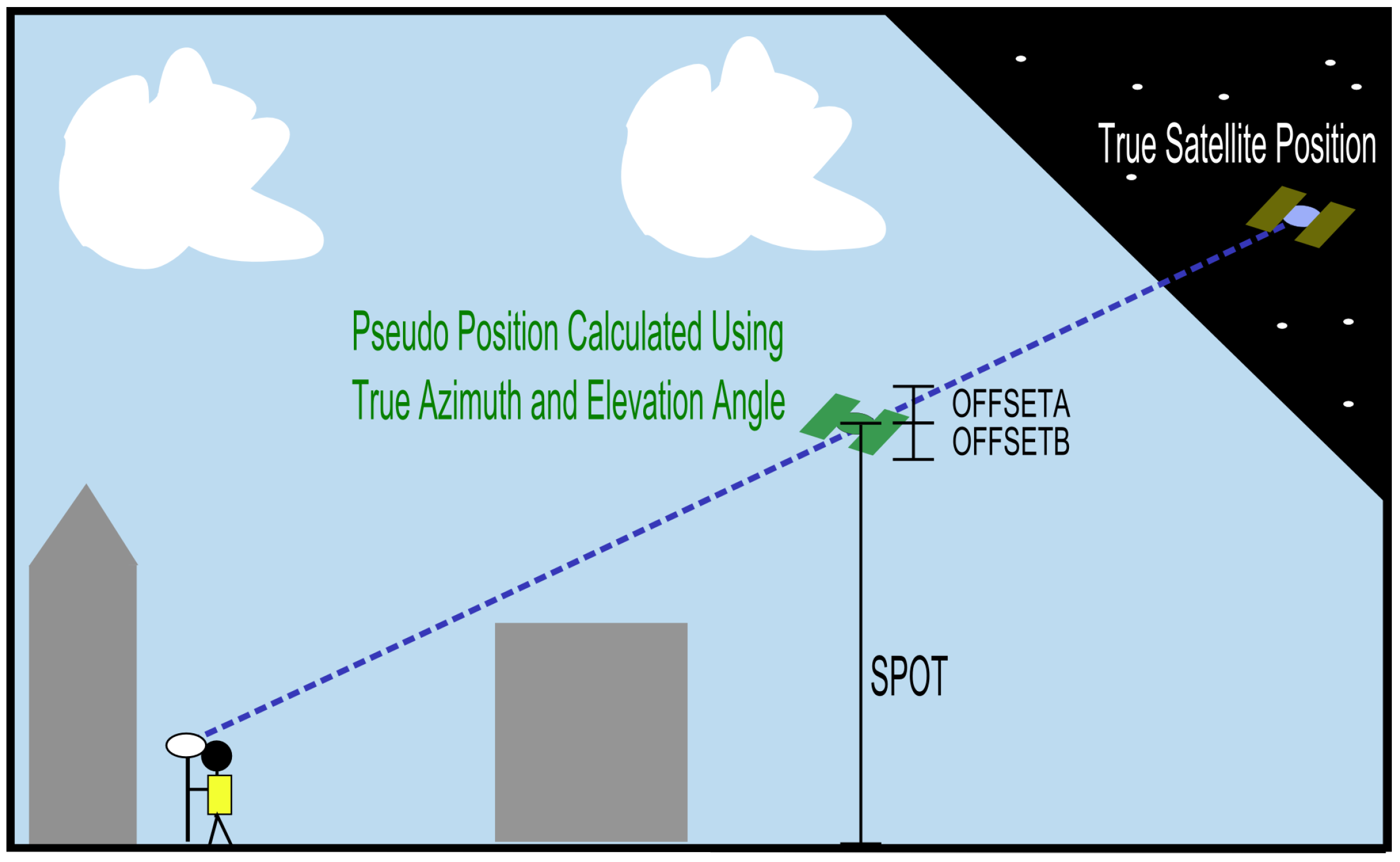
• Reversing output from GNSS shadow prediction tools to calculate pseudo-satellite positions.
• Applying a GIS viewshed with distant observer points in a different coordinate system.

Figure 1. GNSS Survey Planning (a) GNSS signal during topographic surveys can be obstructed by surrounding objects (b) specifying portions of the horizon in Trimble Planning where obstructions are present to simulate buildings or other vertical structures.

Figure 1. GNSS Survey Planning (a) GNSS signal during topographic surveys can be obstructed by surrounding objects (b) specifying portions of the horizon in Trimble Planning where obstructions are present to simulate buildings or other vertical structures.

Figure 2. Mobile Mapping Systems and GNSS Quality (a) the XP1 MMS, designed and developed at the NCG (b) a 2D plot of GNSS satellite signal exhibiting signal loss due to obstructions during an MMS survey.

Figure 2. Mobile Mapping Systems and GNSS Quality (a) the XP1 MMS, designed and developed at the NCG (b) a 2D plot of GNSS satellite signal exhibiting signal loss due to obstructions during an MMS survey.

2. Background and Related Work

The following sections describe the state of the art in three primary components of the methodology, but all are aimed at a single objective—GNSS shadow prediction. An innovative methodology with alternatives to all three components is proposed in this paper and therefore the structure of the discussion must focus on three things required to accurately predict GNSS shadows : information on the obstructions in the area, a method for calculating satellite locations and a method for assessing whether the satellite signal has been obstructed.

2.1. Modelling Obstructions

City models benefit multiple applications such as archaeology [8], transport projects [9], pedestrian behaviour studies [10], Building Information Modelling [11], thermal emissions surveys [12], map updating/change detection [13] or flood defences/town planning [14]. The open standard format, CityGML [15] defines different qualities of structure in terms of the Level Of Detail (LOD), a ranking that goes from 0–4. LOD0 is a 2.5D digital surface model (DSM). An LOD1 city model is a block model without roof structures. LOD2 adds roof forms to each building. LOD3 accurately represents the design and dimensions of each building face and roof, whereas LOD4 also models the interior or each building. The more accurate or realistic the model, the longer it will take to create. This paper will present a method to minimise the time spent creating models for GNSS survey planning.

2.1.1. Modelling with 3D Vectors

Figure 3a, displays a LOD4 model, including interiors and exteriors of Maynooth University created by a team of land surveyors using a terrestrial laser scanner. Traditional survey methodologies such as these [16] or close-range photogrammetry [17] are time consuming and are not readily available for most cities. More rapid methods of surveying urban areas are aerial LiDAR [18], mobile terrestrial LiDAR [19] or earth orbiting satellites. Data from satellites can be used to create 3D models of urban areas, [20] applied an object-based approach to extract buildings from multi-view, high-resolution satellite imagery captured by the PLEIADES constellation. Building height mapping surveys [21], cadastral surveys [22] and deformation studies in urban areas [23] have also been performed using space-borne Synthetic Aperture Radar (SAR) interferometry. The resulting models require powerful workstations to view or manipulate the data. The first innovative element of the novel approach being presented in this paper is a methodology that bypasses the requirement for these high detail models through creation of a 2.5D DSM from 2D vector mapping and low density elevation data at LOD0.

Figure 3. Modelling obstructions (a) a 3D vector model of Maynooth University South Campus created during the 3D Campus project (b) a 2.5D raster DSM of buildings on Maynooth University North Campus created using photogrammetric methods from imagery captured by a Falcon 8 UAV.

Figure 3. Modelling obstructions (a) a 3D vector model of Maynooth University South Campus created during the 3D Campus project (b) a 2.5D raster DSM of buildings on Maynooth University North Campus created using photogrammetric methods from imagery captured by a Falcon 8 UAV.

2.1.2. Modelling with 2.5D Rasters

Although photogrammetric principles applied to imagery captured by manned aircraft [24] are a well practiced method for creating building models for GNSS prediction surveys, it is also possible to model an obstruction using a 2.5D raster DSM (LOD0). Umanned aerial vehicles (UAVs) are now a well established method for creating this type of DSM. Figure 3b displays a DSM of a portion of the North Campus, Maynooth University created using a Falcon 8 Octocopter [25], a Sony Nex-5N SLR and the Pix4Dmapper software [26]. Using 2.5D raster datasets to represent obstructions in an area are a less complex alternative to 3D vector datasets such as the campus model, and UAVs are increasing in popularity among surveyors for topographic and building surveys. Additionally, 2.5D raster datasets are generally much smaller than their 3D vector counterparts and this reduced filesize allows for more efficient processing. Although 2.5D rasters are suitable for GNSS shadow prediction, they still require a survey of the area of interest and subsequent processing to create the DSM. The approach proposed in this paper is a methodology for bypassing the time-consuming aerial survey requirement by employing existing 2D vector data and basic elevation data to create the 2.5D DSM.

2.1.3. Proposed Substitution of 2D Vector Files and Basic 3D Data

In previous GNSS shadowing studies, the importance of using detailed, accurate obstruction models has been emphasised. For example; high accuracy models were used to mitigate multipath in a survey area, improving the navigation solution [27] by minimising the number of false signals reaching the receiver [28]. Fisheye and IR cameras can be used to remove non-visible satellites in the position calculation, through post-processing or even in real-time [29,30] and these methods are independent of city models. When detailed obstruction models are employed, they are created through simulation [31] or by survey [32]. In [33], polyline shapefiles containing one-foot bare-earth elevation, contours were used and building roof and ridge outlines and elevations were manually digitized.

However, due to the cost of surveying an area, processing the data and creating the models, there is a strong justification for developing a method that can take advantage of existing national mapping such as Ordnance Survey Ireland (OSi) 2D digital vector mapping and any available elevation information. This type of mapping is available to most government agencies and other public bodies and is therefore a ready source of mapping for GNSS predictions. It is one of the goals of this paper to demonstrate that the proposed method of converting 2D vector mapping and basic elevation data into a raster DSM is a practical alternative to surveying the area. Basic elevation data can be acquired from low density aerial surveys, satellite imagery or alternatively, information on building heights available from Town Planning Department or Land Registry databases usually reserved for planning appeals, property registration or “right to light” appeals. This combination of 2D polygons and sparse elevation data yielded promising results when applied in [34] to facilitate automatic extraction of objects from LiDAR data. The proposed methodology will be employed to avoid the need for costly, time-consuming surveys and intensive computer processing.

2.2. Satellite Location

As previously stated, existing software packages provide a method for calculating satellite visibility at a single location, at any time and this software provides detailed information on the orbital information of GNSS satellites. Another method for survey planning is to design a programme which can track satellite positions at all times, such as those employing a two-line element set (which describes the orbits of earth-orbiting satellites) as proposed by [33] or the Keplerian parameters used in the GRASS module employed by [35]. These methods are heavy in terms of computational performance but will provide the user with real-time information on satellite position. An alternative is to use a simulated GNSS constellation, such as that employed by [31,36]. The innovative method proposed in this paper utilises freely available planning software such as Trimble Planning, and then reverses the satellite prediction algorithm output. Instead of calculating the number of satellites visible at the receiver, the proposed method calculates a pesudo position for the satellite while simultaneously maintaining its correct azimuth and elevation. This approach is enabled through a basic HTML editor, the output of the Trimble Planning desktop application, and provides savings in terms of processing time.

2.3. Visibility Calculation in a GIS

Certain applications benefit from GNSS shadows, for example, [31,32] predict what satellites should not be visible from different locations and then use these shadows to calculate receiver position during a survey. However, the goal of this paper is to assist the surveyor in avoiding GNSS shadows when planning the survey, particularly for mobile surveys. In this study, a GIS has been applied to help with calculating satellite visibility.

Using a GIS to model line of sight/pathing is not a novel concept, as this capability has been used for many applications including archaeology [37], least-cost path analysis [38] and intercepting solar radiation [39]. One method is to employ the ArcMap line-of sight (LOS) tool. The LOS tool requires that you specify two points on a line, the first and last vertex. One is the observer, one is the target and then visibility is calculated through ray tracing (a method recently applied in a study for satellite visibility using Google Earth [40]). Calculating GNSS shadows over a wide area requires each satellite to be modelled and the line of sight calculated for every possible surveyor position in the area. In [18], the authors designed a system to encompass the whole GNSS satellite range, used airborne LiDAR to create a 3D city model of a city and the 3D Analyst Line of Sight tool to calculate visibility. In their work on satellite visibility, [24] also applied the 3D Analyst Line of Sight tool. In [35], the authors applied the r.obstruction and r.planning.static modules in GRASS for their work on GNSS planning.

To improve on this, the final novel element of the proposed methodology is to apply the viewshed algorithm from ESRI ArcMap, thereby negating the requirement for each observer/target point to be specified. A viewshed calculates each target cell in a raster that can be seen from multiple observation locations, which in in this case are the satellites. Each pixel in the output image then stores a value of how many observer points can be seen from that position. In [33], the authors highlighted that the primary restriction of the ArcMap viewshed tool that prevents it from being used for satellite visibility prediction is that the observer points (satellites) cannot be thousands of kilometres from the test area and in a different coordinate system. The novel methodology proposed in this paper of using a pseudo satellite position created from the true bearing and azimuth enables the circumvention of these restrictions.

3. Datasets

Four datasets were used in this study. These were the GNSS almanacs incorporated in Trimble Planning, a 3D model of Maynooth University south campus created with a terrestrial laser scanner (but only used as an available source of individual elevation values for the buildings on campus), OSi vector mapping and topographic survey data captured with a GNSS receiver that was used in the validation tests.

3.1. GNSS Almanac/Trimble Software

Accurate information for satellite positions at different times of the day was required. As previously demonstrated, a number of different methods are available that detail the orbit precisely. If kept up to date, these software tools can be used to calculate the position of any GNSS satellite at any time of day. However, this is a complicated process in terms of user training and also in terms of processing time. It was one of the aims of this study to show that an existing, free GNSS software package was a suitable substitute, providing savings in terms of cost and time. Trimble Planning was readily available; therefore, this method could be more readily reproduced and so was selected for the project. This study was limited to GPS and GLONASS satellites only as the GNSS receiver used in the validation tests was limited to those constellations.

3.2. OSi Digital Mapping

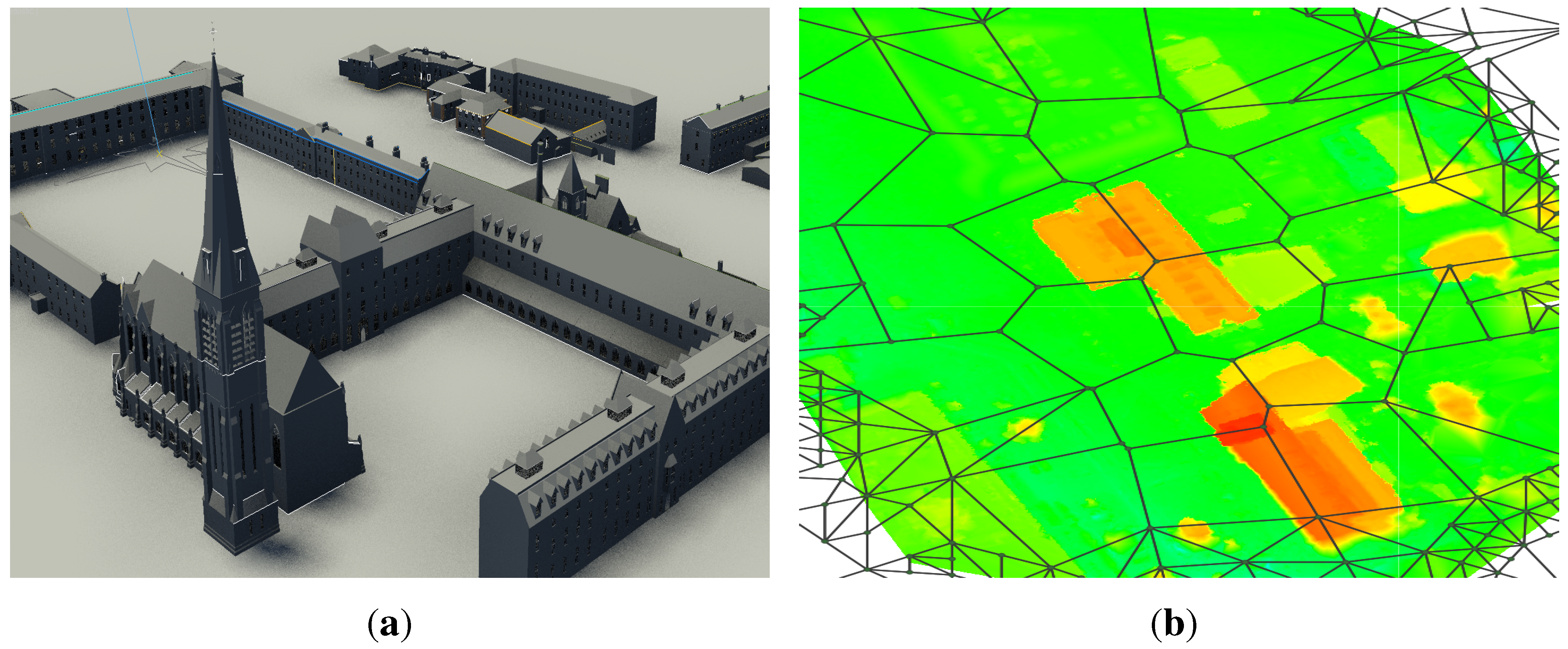
A typical example of vector mapping such as the OSi digital mapping of Maynooth University (Figure 4a) provides any potential user with a quick method of acquiring building footprint polygons and was incorporated into this project. The vector mapping was edited using Bentley’s MicroStation V8 [41], a popular CAD environment. For this project, all mapping layers (e.g., water, infrastructure, legal boundaries) with the exception of the building footprints were removed, as illustrated in Figure 4b where the single building layer has been isolated. If this process was expanded to a larger area involving hundreds of digital mapping tiles, this process could be streamlined by specifying a single layer and running a batch process to extract the relevant layer. These building polygons were created from aerial photography and have a quoted accuracy of approximately ±0.60 m [42].

Figure 4. Ordnance Survey Ireland 2D vector mapping (a) all layers active in the test area viewed in a CAD environment (b) building footprint layer isolated for obstruction modelling.

Figure 4. Ordnance Survey Ireland 2D vector mapping (a) all layers active in the test area viewed in a CAD environment (b) building footprint layer isolated for obstruction modelling.

3.3. 3D Campus

This extremely high density and high accuracy survey data was captured using a Leica HDS3000 and compiled using Leica’s Cyclone [43] and Autodesk’s 3D Studio [44]. 3D Studio is a professional 3D modelling package used for dealing with large volumes of points, and the high quality of the models can be seen in Figure 3a. As we are proposing the alternative method of using the OSi 2D vector data, the campus 3D model was not used to model obstructions but used solely to ascertain a single, individual, accurate elevation value for the footprint and roof of every 2D building polygon. Single elevation values were used to replicate an aerial LIDAR point cloud, and other low-density datasets or values from an existing database.

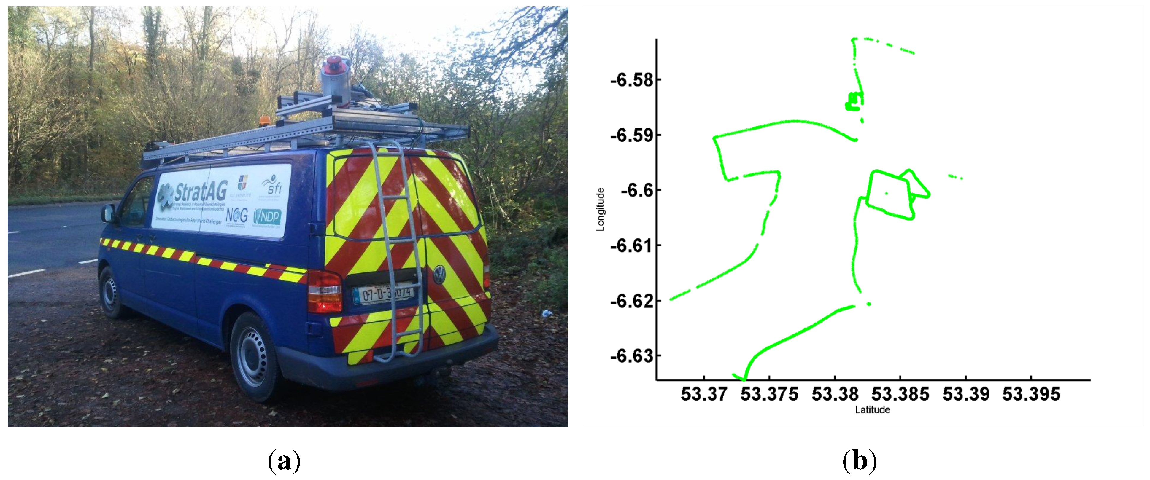
3.4. Trimble R8 GNSS Survey Data

A Trimble R8 GNSS receiver [45] was used in the validation tests in this paper. The R8 is a survey grade GNSS rover and is capable of calculating position based on signals from both the GPS and GLONASS constellations. Receivers that can record signals from multiple constellations increase the number of satellites available for a surveyor at any time of day. The receiver was positioned at multiple locations around Maynooth University South Campus for the accuracy tests. A bi-pod was used to minimise any receiver motion during the validation measurements. The user interface on the data-logger displays the number of satellites visible to the receiver at the current time and this was used to validate the prediction results.

4. Methodology

This study involved five distinct stages. The first of these was calculating the satellite positions over Maynooth University, the second involved extracting 2D polygons of the campus, followed by creation of a surface model of the campus. In the fourth stage, the 3D Analyst viewshed functions were applied to ascertain visibility and, in the final stage, the accuracy of the prediction results were assessed.

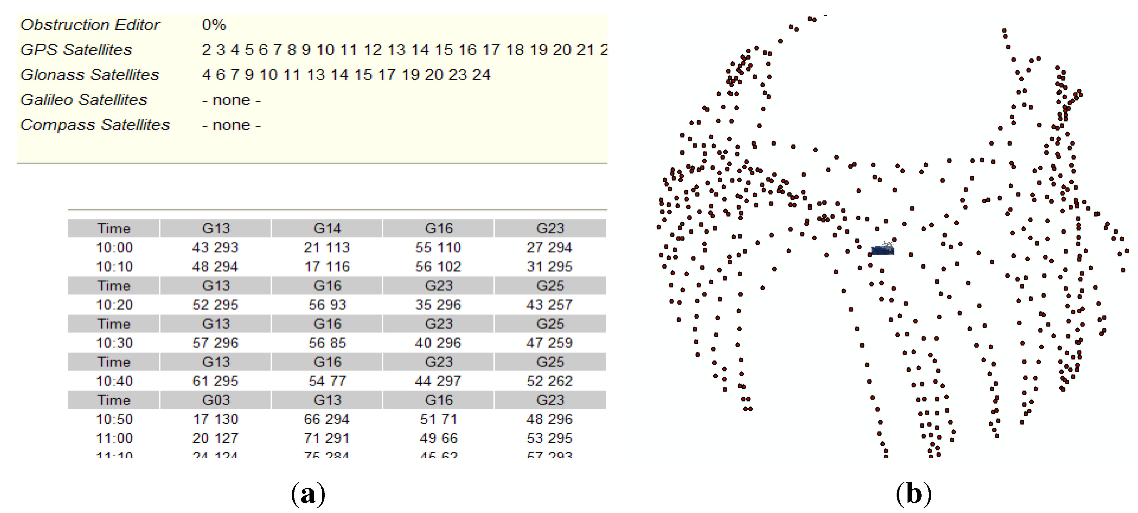
4.1. Calculate Satellite Positions

It is essential for accurate satellite prediction surveys that the position of GNSS satellites in any constellation can be calculated at all times. The satellite ephemeris data (containing positional data, orbital information and satellite health) is broadcast in an almanac and this can be downloaded. Occasionally, there are adjustments to satellite orbits, so these almanacs must be kept updated. Importantly for the proposed methodology, software such as Trimble Planning also provides information on the azimuth and elevation to each satellite from a known observer point in the prediction results. Using this information to calculate pseudo satellite positions enabled us to avoid the need for a coordinate transformation from the earth-centred coordinate system of latitude and longitude to the projected coordinate system of the OSi digital mapping best suited for GNSS surveys [46], the Irish Transverse Mercator (ITM). To ensure the simulated satellites were not too close to the survey site (which would mean they would have an exaggerated field of view), they were simulated at a distance of 10 km from the campus. This simulated value was required in calculating the simulated coordinates. By developing a method that incorporates a pseudo distance that is shorter than the true distance, it allows us to avoid the viewshed restrictions identified by [33].

For the initial tests, one day was chosen for the study and the time of the test was limited to between 10:00 and 17:00. A single point was selected in the centre of the campus and a table of all visible satellites and their elevations and azimuths at ten minute intervals from 10:00 to 17:00 was created (Figure 5a). In this image, the numbers in the table below each satellite ID refer to the elevation (always less than 90${}^{\circ }$) and the azimuth (between 0${}^{\circ }$ and 360${}^{\circ }$). One issue with this process is that the Trimble Planning software only allows the latitude/longitude of the observer point to be specified in degrees and minutes, rather than degrees, minutes and seconds. This lowered the accuracy when specifying the position of the observer point, but planning of GNSS surveys does not require a high accuracy in positioning the single observer point and only influences the result when the point occurs close to the transition between two minutes (i.e., at 59 seconds.

Figure 5. Calculating satellite positions (a) prediction results from Trimble Planning for 10 min intervals over the test site (b) a 2D plot of pseudo satellites positions at 10 min intervals over Maynooth University between 10:00 and 17:00.

Figure 5. Calculating satellite positions (a) prediction results from Trimble Planning for 10 min intervals over the test site (b) a 2D plot of pseudo satellites positions at 10 min intervals over Maynooth University between 10:00 and 17:00.

The data was exported into HTML format and then accessed and edited using an HTML editor. The geometric formulae for transforming coordinates X,Y and Z respectively to their pseudo positions X’, Y’ and Z’ given the 10 km simulated range (s) and the measured azimuth (θ) and elevation (ϕ) calculated by Trimble Planning were

$$X^{\prime }=s(cos\varphi \times sin\theta )$$

(1)

$$Y^{\prime }=s(cos\varphi \times cos\theta )$$

(2)

and

$$Z^{\prime }=s(sin\varphi )$$

(3)

This data was collated in a table and imported into ArcMap. An SQL query enabled the satellites present at any time of the day to be identified, isolated and visualised for analysis in the GIS. Figure 5b displays a 2D plot of all of the satellites from the GNSS constellations that were present over Maynooth University on Wednesday, 4th May between 10:00 and 17:00 visualised in ArcMap.

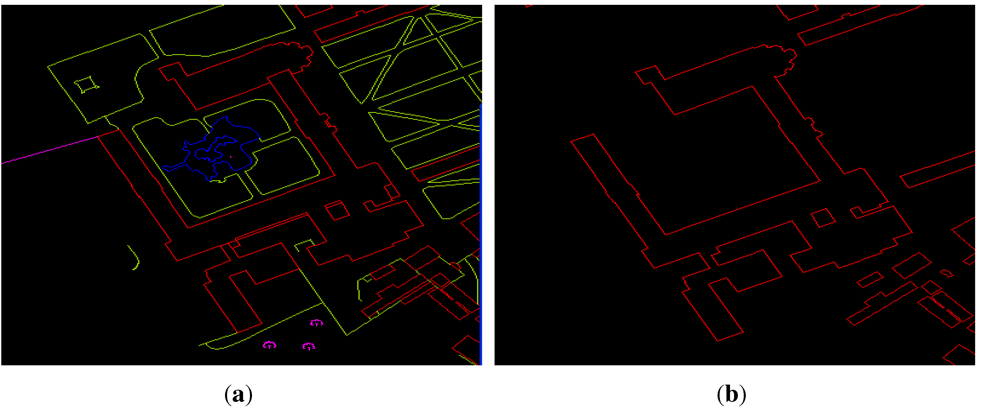
4.2. Extract 2D Vector Building Polygons

Crowd-sourced datasets were initially investigated as a cost-effective solution for providing 2D polygons. For example, Open Street Map (OSM) building polygons could be used if the accuracy was sufficient; however, studies [47] have shown that the mean error between OSM and accurate reference data is 6.65 m and the maximum error can be as high as 31 m. This accuracy is clearly not sufficient for GNSS predictions surveys and therefore OSi digital mapping was selected to demonstrate the methodology. Although it is used under licence and, therefore, there is a cost involved, vector datasets such as these are a popular and accurate source of mapping in many countries, whether designed for fixed boundary, high accuracy cadastral mapping (Germany, Denmark) or non-conclusive boundary registration systems like Ireland [48].

Using existing mapping avoids the need to pursue the time-consuming process of digitising each building from raster imagery or performing a topographic or aerial survey. All features except buildings were removed and the 2D polygons on the building layer were then imported into ArcMap. One issue with using the building polygons was that trees, street furniture and other infrastructure were not included. Trees are an important factor in GNSS prediction as they block satellite signals, particularly in the spring or summer as the vegetation canopy thickens, however surveying and digitising each tree on campus would be too time-consuming, and it was an important goal of the proposed methodology to avoid the need for pre-surveying an area.

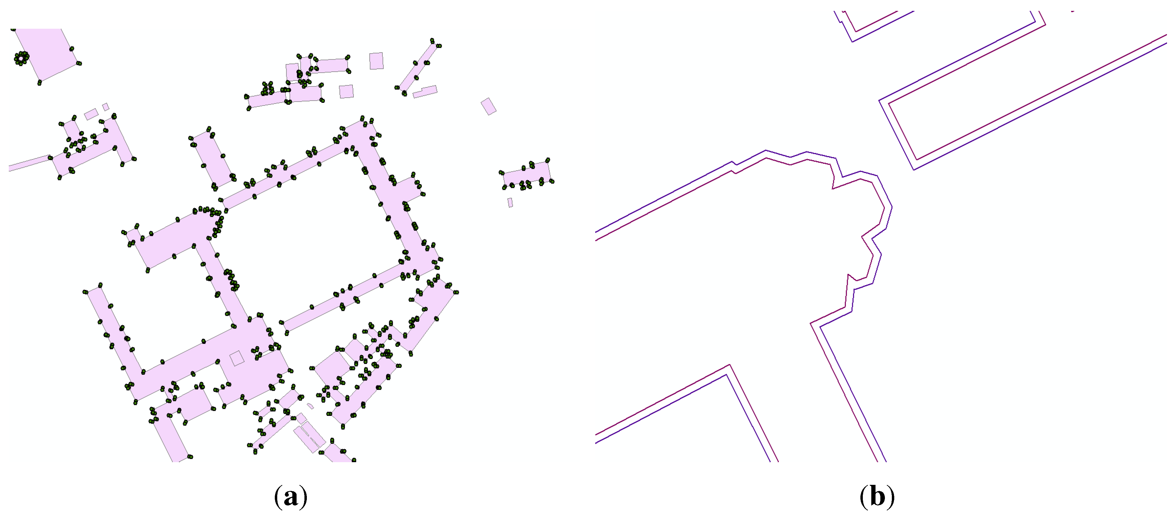
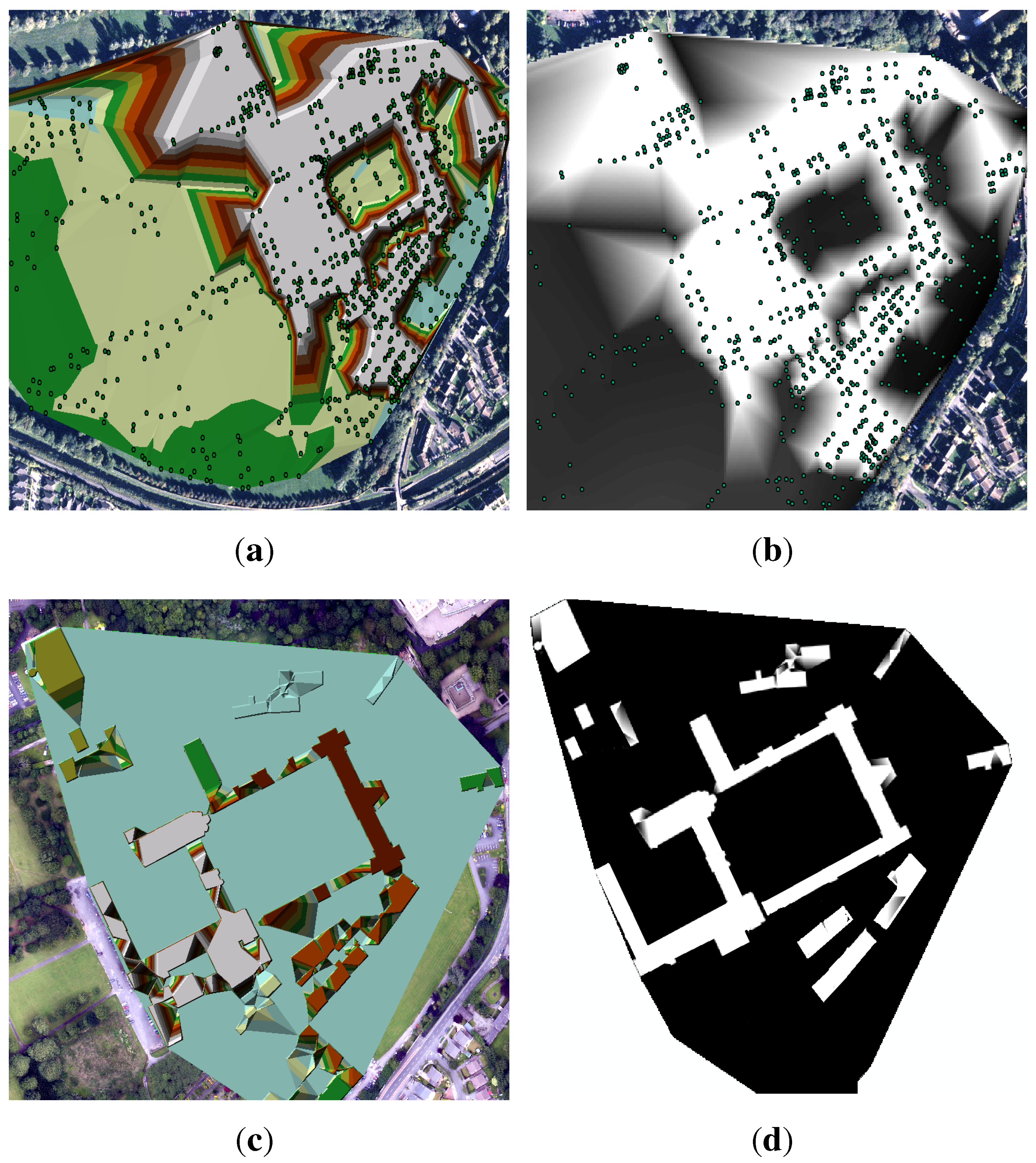
4.3. Create 2.5D Raster Campus

A number of steps were involved to create a 2.5D raster surface model of the buildings on campus to use with the viewshed calculation. First, each of the 2D building polyons were assigned height values. Using the, ArcMap “feature to ascii” tool the XY values for each of the polygon vertices (Figure 6a) were exported into a table and a single Z value from the 3D campus model was assigned to every vertex of a building polygon. As previously explained, by demonstrating that combining 2D vector data with a single elevation value for each building was a suitable substitute for a high density 3D model, it could potentially provide savings in term of survey time, processing time and cost.

These points were then used to create a Triangulated Irregular Network (TIN) as it is the first step in the creation of a raster DSM for use in the visibility calculation in ArcMap. The TIN process joins all adjacent XYZ points in a network of non-overlapping triangles, but it has difficulties when there are points on top of each other (i.e., identical XY coordinates but different Z coordinates) and for this reason a short, 1 m offset (Figure 6b) was incorporated for each building footprint. Once the XYZ values for each polygon vertex were found, the original polygons and the offset polygon were combined so the TIN could be created. The problem presented if the offset was omitted is apparent when the TIN (Figure 7a) and resulting raster DSMs were created (Figure 7b) as there were minimal elevation changes between the majority of surfaces. However, after the 1 m buffer was applied, this resulted in a greatly improved TIN for the buildings on campus (Figure 7c) although certain problematic areas still existed due to issues with the building footprint offsets whereby the building is flagged as larger than it should be. Basic editing of problematic triangles allowed creation of an improved raster DSM (Figure 7d) and this 2.5D raster DSM, created using 2D vector data and basic elevation information, was used to model obstructions in the viewshed calculation. Experimentation with different buffer distances could improve DSM creation, benefiting future applications of the methodology if upscaling to larger test areas.

Figure 6. Processing the 2D vector polygons (a) identifying the X ,Y coordinates of each building polygon vertex (b) applying a 1 m offset to the polygons to aid in triangulated irregular network creation.

Figure 6. Processing the 2D vector polygons (a) identifying the X ,Y coordinates of each building polygon vertex (b) applying a 1 m offset to the polygons to aid in triangulated irregular network creation.

4.4. 3D Analyst Viewshed GIS Calculation

The ArcMap viewshed tool calculates visibility from an observer point (in this case the satellites) to a surface (the campus raster DSM). One restriction is that the objects must be in the same coordinate system; however, the novel methodology of calculating pseudo satellite positions proposed in this paper has enabled its application. Although the viewshed tool can incorporate earth curvature, the satellites visible to a surveyor will all be above the horizon and as no DSM for the areas outside the campus was used, all positions could be considered relative to the local plane. The first required field in the viewshed tool, SPOT (Figure 8), dictates the elevation of the observer point. In this case, SPOT was set to be the pseudo Z value of the satellite, Z’. Other optional fields were OFFSETA and OFFSETB. OFFSETA can be employed when modelling visibility of wind farms, radio masts or similar vertical structures as it allows a height value for of the structure to be defined. OFFSETA was set to an arbitrary low value of 1 m. OFFSETB allows a negative vertical height to be defined and was not required, therefore OFFSETB was left blank. Additional optional fields of AZIMUTH, VERT, RADIUS and YY were not included, as these are only required when the field of view or viewing range of the observer points are to be restricted. In this study, it was not, and by excluding these fields it defaults to the maximum value, i.e., a 0${}^{\circ }$–360${}^{\circ }$ search in azimuth and vertical of unlimited range. If trying to increase processing times in future tests, this could be achieved by excluding all objects above the satellite. Specifying the time of day that satellite visibility over Maynooth Campus was done using an SQL statement. After this, the obstruction surface was applied and the viewshed calculated. Although five satellites are generally required for most satellite receivers in RTK mode, four is the mathematical minimum and this was applied as the lower cut-off for these tests. These two classes gave a definite yes/no answer for satellite visibility.

Figure 7. Creating surfaces to model obstructions (a) TIN without 1 m offset exhibits poor definition of elevation changes (b) low quality raster DSM created using TIN without 1 m offset (c) 1 m offset results in an improved TIN (d) improved TIN results in an improved raster DSM.

Figure 7. Creating surfaces to model obstructions (a) TIN without 1 m offset exhibits poor definition of elevation changes (b) low quality raster DSM created using TIN without 1 m offset (c) 1 m offset results in an improved TIN (d) improved TIN results in an improved raster DSM.

Figure 8. Creating a viewshed observer point using the pseudo satellite position.

Figure 8. Creating a viewshed observer point using the pseudo satellite position.

5. Results and Discussion

The following sections present the results of the GNSS prediction methodology. Additionally, a procedure for validating these predictions using true values was designed. A GNSS receiver was used to measure the number of satellites visible at a number of distinct locations on Maynooth University campus and this validation data was then compared with the predicted values and the error sources were explored. This enabled assessment of the proposed methodology of applying existing prediction software, 2D polygons and low-density elevation data in ArcMap’s viewshed analysis.

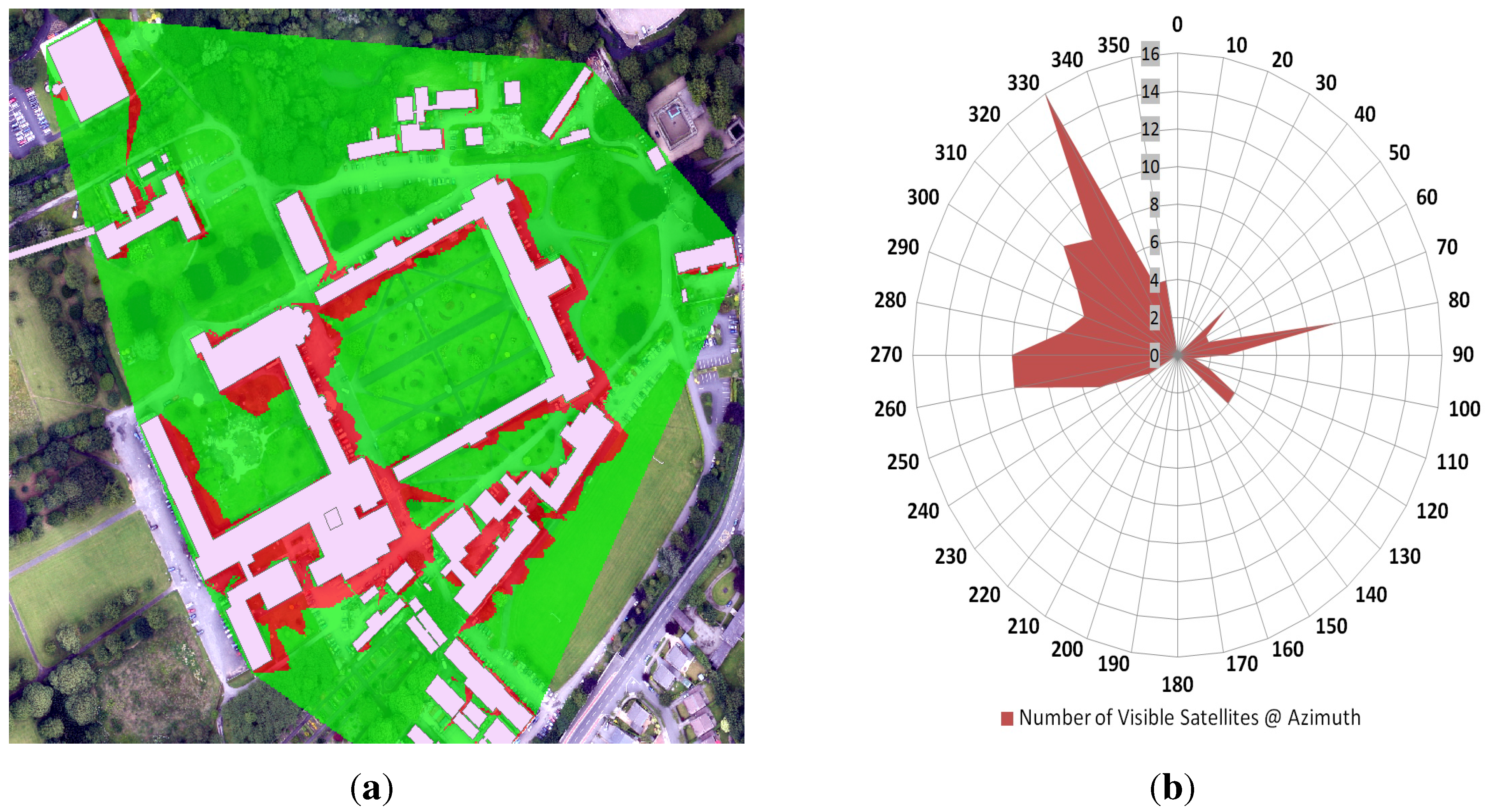
5.1. Interpretation of GNSS Prediction Results

The results of the viewshed analysis for a single point in time at Maynooth University are displayed in Figure 9a. This image displays the output from the proposed satellite visibility methodology after obstructions have been included. The 2D vector polygons representing the building footprints have been included as an aid to visualising these obstructions when interpreting the results. Areas in green represent areas of four satellites or more whereas areas in red are areas visible to fewer than four satellites, implying that a GNSS receiver would not be capable of calculating an accurate 3D position at that location. Upon examining the results a very definite trend towards GNSS shadows in the south and southeast of the buildings was apparent, with tall buildings exhibiting longer shadows than smaller buildings. This overall trend in shadow distribution implies that the satellite constellation was primarily in the north and northwest at the time of the survey. This assumption was verified when a plot of satellite azimuth throughout the prediction tests was created (Figure 9b), with the majority of GNSS satellite orbits visible from the quadrant of azimuth of 270${}^{\circ }$–350${}^{\circ }$. The values on the Y axis represent the total number of satellites measurements recorded at that azimuth throughout the tests—for example, 141 satellite positions were recorded throughout the tests and approximately 95 of those observations were positioned at azimuths of 270${}^{\circ }$–350${}^{\circ }$ from the observer position. An initial examination of the shadows in the test area suggest that the method has successfully modelled the obstructions in the area:

• The long slender shadow to the south of the central courtyard in the prediction results was caused by the tall spire of the cathedral on campus, which is over 80 m in height.
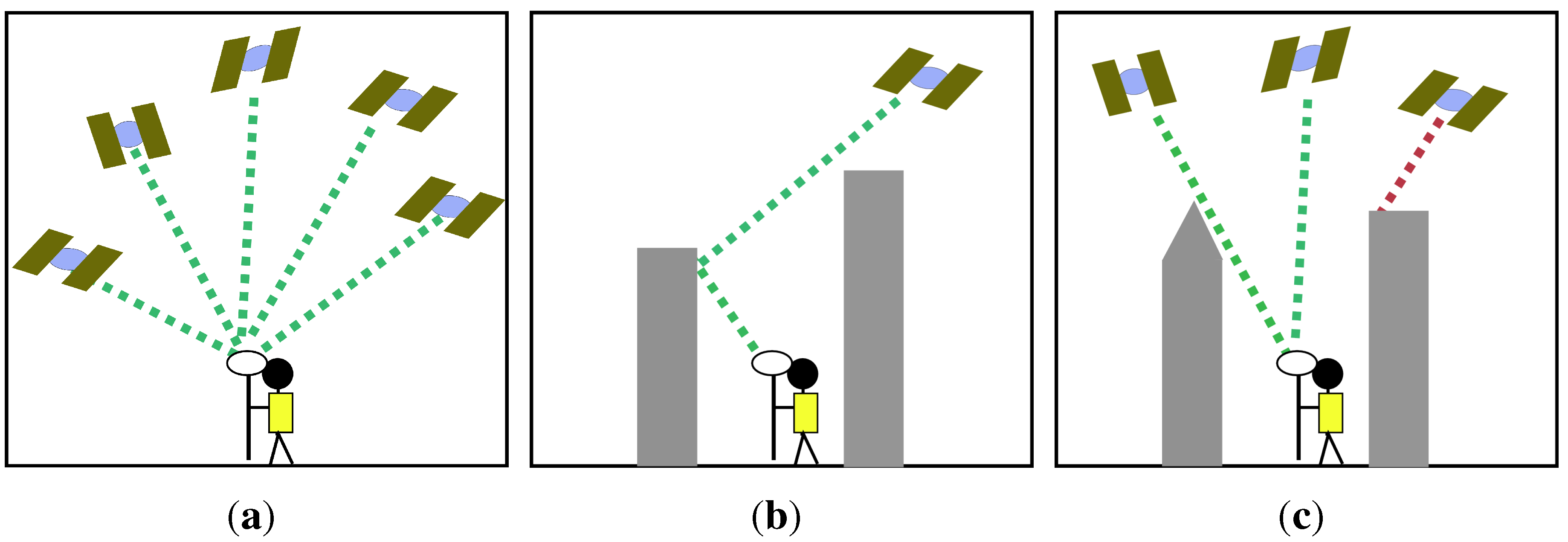
• Areas of the smaller courtyards were almost completely in shadow, implying that if a surveyor were operating in that area they would find it extremely difficult to acquire any GNSS signal, as would be expected in real life.

The cause and shape of other GNSS shadows, such as the long, slender shadow in the northwest of the map were more difficult difficult to identify:

• This shadow was potentially caused by a satellite in the southwest of the area that eliminated a shadow close to the building or a satellite high in the horizon in the northwest that was able to view part of the southern face of the building, thus eliminating the rest of the shadow in this area. Figure 9b proves that there were satellites in the southwest throughout the survey.
• Alternatively, there could be an error in the TIN in this area, as this building exhibited a triangular extension in Figure 7c. This was not apparent in the resulting raster DSM, however, so the ultimate cause is uncertain.

Figure 9. Results and accuracy Tests (a) visualising output from the proposed methodology—green areas: visible to four plus satellites, red: less than four satellites (b) a plot of satellite azimuths throughout the validations tests—red represents azimuth and number of satellites, grey numbers on Y axis represent total number of satellites visible from the observer location throughout the tests.

Figure 9. Results and accuracy Tests (a) visualising output from the proposed methodology—green areas: visible to four plus satellites, red: less than four satellites (b) a plot of satellite azimuths throughout the validations tests—red represents azimuth and number of satellites, grey numbers on Y axis represent total number of satellites visible from the observer location throughout the tests.

Figure 10. Validation tests (a) validation points selected as representative of the surrounding environment (b) azimuth of the two predominant shadowing objects throughout the validation tests at each of the ten test locations.

Figure 10. Validation tests (a) validation points selected as representative of the surrounding environment (b) azimuth of the two predominant shadowing objects throughout the validation tests at each of the ten test locations.

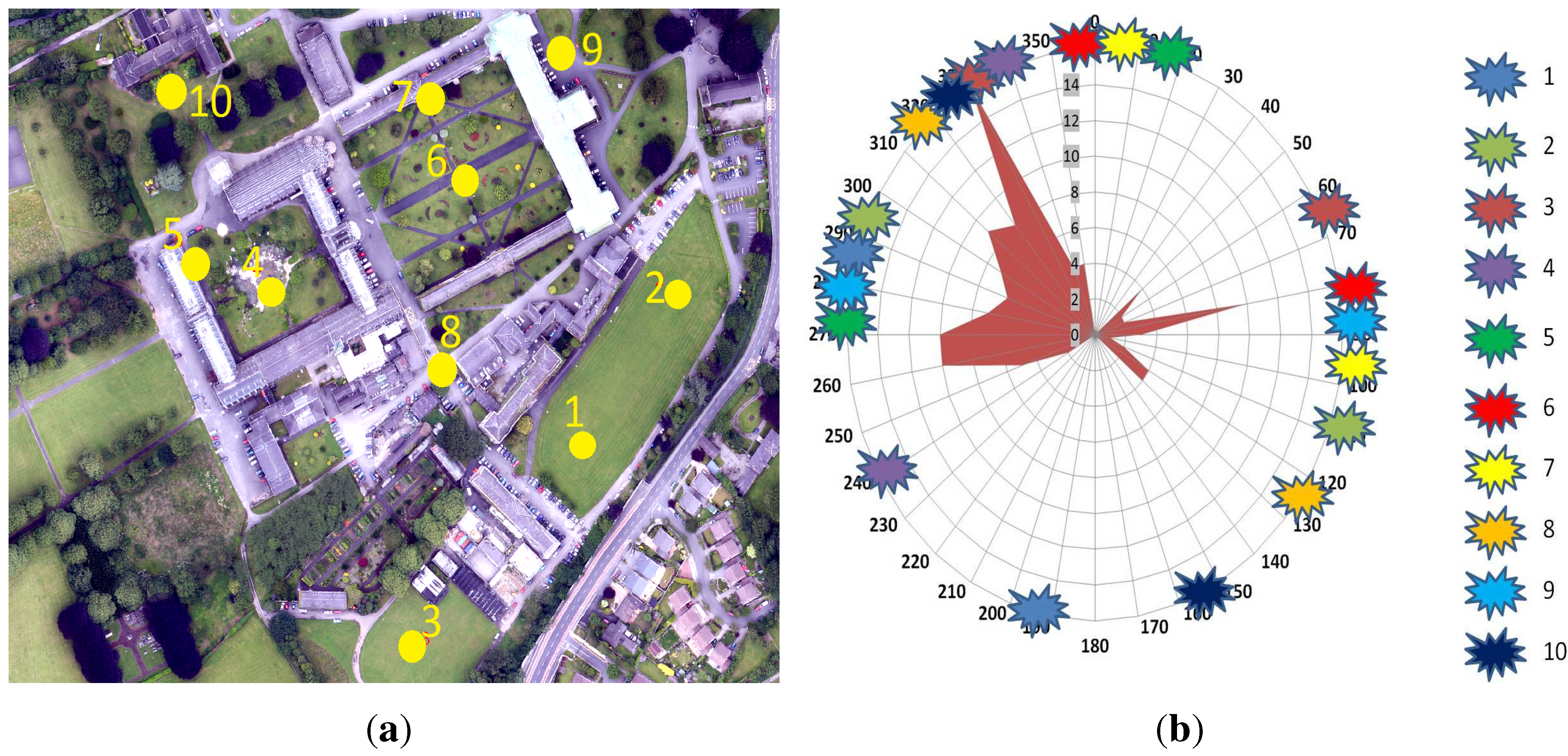
5.2. Choice of GNSS Sample Locations

To assess the accuracy of the GNSS shadow prediction methodology, all satellites visible to a Trimble R8 GNSS receiver were counted at various times and locations on campus. A number of representative points were selected to ensure shadowing of the receiver in at least one quadrant for every test. Figure 10a displays the selected locations for the validation tests. Locations such as an open space, a courtyard, a narrow access route between two buildings and four points adjacent to large obstructions to the N,S E and W were chosen. Figure 10b graphically displays the azimuth of the two dominant sources of shadow for each check point, numbered 1–10 and these coincide with the test locations marked in Figure 10a. An additional limiting factor when choosing the sampling-locations was vegetation. Because vegetation was not incorporated in this iteration of the methodology, sites with large amounts of vegetation were avoided when possible. The vegetation was predominantly located in the west of the campus as illustrated in Figure 10a.

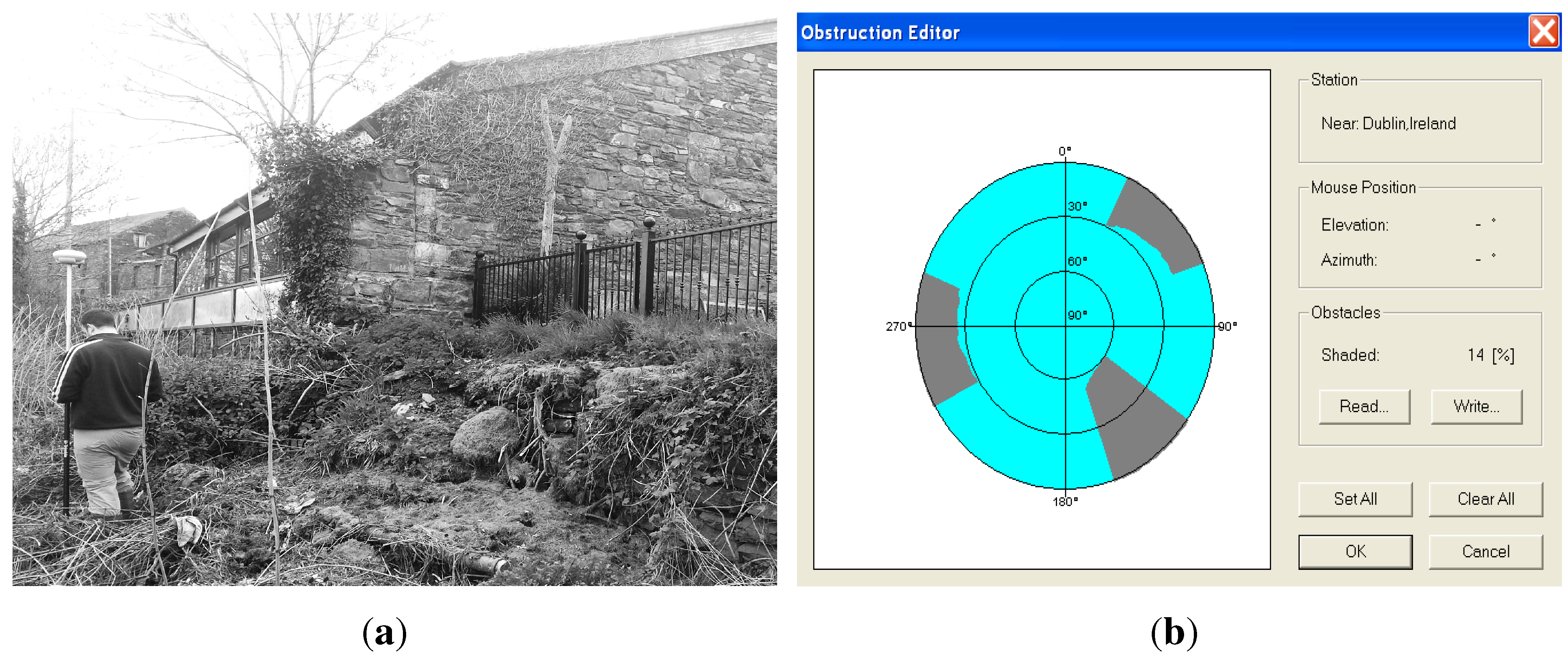
5.3. Validation of the Methodology

Due to the requirement for manual validation at each location, these tests could not be performed simultaneously with a single receiver and therefore the number of satellites changed during the tests. The satellite visibility calculation was repeatedly updated to coincide with each recorded checkpoint. Table 1 lists the terminology used in the validation and analysis.

Table 1. Global navigation satellite system (GNSS) prediction validation test terminology.

Term	Definition
$Tota{l}_{\mathrm{sat}}$	Number of satellites predicted at the receiver location assuming no obstructions.
$Predicte{d}_{\mathrm{obs}}$	Number of satellites predicted once obstructions have been included.
$Measure{d}_{\mathrm{obs}}$	Number of satellites observed once obstructions have been included.
$Error$	Discrepancy between $Predicte{d}_{\mathrm{obs}}$ and $Measure{d}_{\mathrm{obs}}$.

Table 1. Global navigation satellite system (GNSS) prediction validation test terminology.

Term	Definition
$Tota{l}_{\mathrm{sat}}$	Number of satellites predicted at the receiver location assuming no obstructions.
$Predicte{d}_{\mathrm{obs}}$	Number of satellites predicted once obstructions have been included.
$Measure{d}_{\mathrm{obs}}$	Number of satellites observed once obstructions have been included.
$Error$	Discrepancy between $Predicte{d}_{\mathrm{obs}}$ and $Measure{d}_{\mathrm{obs}}$.

Upon comparing the maximum, the predicted and the observed number of satellites visible at each location, the promising results appear to validate the methodology. Table 2 displays these results. The largest discrepancy between $Predicte{d}_{\mathrm{obs}}$ and $Measure{d}_{\mathrm{obs}}$ was an over-prediction of two satellites at Point 3. There is an avenue of large trees lining the walled garden to the North West of this test location and another avenue of large trees lining the University boundary to the East. The lack of vegetation in the model has caused errors in this prediction instance. At six of the ten test-sites (Points 4, 5, 6, 7, 8 and 10) the $Predicte{d}_{\mathrm{obs}}$ value was identical to the validation, $Measure{d}_{\mathrm{obs}}$, i.e., the proposed method has returned a zero error for 60% of the tests. The results from Points 5, 7 and 10 are particularly promising as they were all located in close proximity to a tall building and therefore experienced severely restricted GNSS visibility.

Table 3 lists the error in prediction and the azimuth of the two dominant sources of shadow for each point, the range to those obstructions and the height of each obstruction (also displayed graphically in Figure 10b). Each obstruction is also identified in Table 3. The correct number of satellites at 5, 7 and 10 was calculated when the range to the building varied between 2 m and 5.6 m and also calculated at Point 8, which was positioned at a junction between large buildings. Accurately predicting GNSS visibility in problematic areas such as these implies that our approach of modelling obstructions and predictions using existing software, 2D polygons and low-density elevation information was successful.

Table 2. GNSS prediction validation test results, description of site and shadowing objects.

Point	Time	$Tota{l}_{\mathrm{sat}}$	$Predicte{d}_{\mathrm{obs}}$	$Measure{d}_{\mathrm{obs}}$	$Error$	Location	Shadowing Objects
1	10:24	9	9	8	1	Pitches	Buildings
2	10:26	9	9	8	1	Pitches	Buildings, Trees
3	10:31	10	9	7	2	Open Space	Trees
4	10:39	10	8	8	0	Courtyard	Buildings, Spire
5	10:41	9	2	2	0	Courtyard	Buildings, Spire
6	10:45	9	9	9	0	Square	Buildings, Spire
7	10:47	9	4	4	0	Square	Buildings
8	10:55	10	2	2	0	Junction	Buildings, Spire
9	11:03	10	5	4	1	Car Park	Buildings , Trees
10	11:17	11	1	1	0	Open Space	Building, Trees

Table 2. GNSS prediction validation test results, description of site and shadowing objects.

Point	Time	$Tota{l}_{\mathrm{sat}}$	$Predicte{d}_{\mathrm{obs}}$	$Measure{d}_{\mathrm{obs}}$	$Error$	Location	Shadowing Objects
1	10:24	9	9	8	1	Pitches	Buildings
2	10:26	9	9	8	1	Pitches	Buildings, Trees
3	10:31	10	9	7	2	Open Space	Trees
4	10:39	10	8	8	0	Courtyard	Buildings, Spire
5	10:41	9	2	2	0	Courtyard	Buildings, Spire
6	10:45	9	9	9	0	Square	Buildings, Spire
7	10:47	9	4	4	0	Square	Buildings
8	10:55	10	2	2	0	Junction	Buildings, Spire
9	11:03	10	5	4	1	Car Park	Buildings , Trees
10	11:17	11	1	1	0	Open Space	Building, Trees

Table 3. Details of the two predominant shadowing objects at each GNSS validation point.

Observations		Shadow Object 1			Shadow Object 2
Point	Error	Azimuth	Height	Range	Azimuth	Height	Range
1	1	195${}^{\circ }$	13.8 m	30.6 m	283${}^{\circ }$	12.7 m	45 m
2	1	287${}^{\circ }$	9.6 m	23.5 m	110${}^{\circ }$	Veg	33.9 m
3	2	65${}^{\circ }$	13.8 m	75 m	340${}^{\circ }$	Veg	18.7 m
4	0	345${}^{\circ }$	76.5 m	67.5 m	295${}^{\circ }$	5 m	20 m
5	0	17${}^{\circ }$	76.5	39.3 m	270${}^{\circ }$	24 m	2 m
6	0	75${}^{\circ }$	14.4 m	49.3 m	0${}^{\circ }$	14.4 m	40.5 m
7	0	0${}^{\circ }$	14.4 m	2 m	90${}^{\circ }$	14.4 m	54.8 m
8	0	325${}^{\circ }$	8 m	40.4 m	125${}^{\circ }$	12.7 m	39.3
9	1	270${}^{\circ }$	14.4 m	5.6 m	90${}^{\circ }$	Veg	22.6 m
10	0	342${}^{\circ }$	7.5 m	4.6 m	156${}^{\circ }$	Veg	12.5 m

Table 3. Details of the two predominant shadowing objects at each GNSS validation point.

Observations		Shadow Object 1			Shadow Object 2
Point	Error	Azimuth	Height	Range	Azimuth	Height	Range
1	1	195${}^{\circ }$	13.8 m	30.6 m	283${}^{\circ }$	12.7 m	45 m
2	1	287${}^{\circ }$	9.6 m	23.5 m	110${}^{\circ }$	Veg	33.9 m
3	2	65${}^{\circ }$	13.8 m	75 m	340${}^{\circ }$	Veg	18.7 m
4	0	345${}^{\circ }$	76.5 m	67.5 m	295${}^{\circ }$	5 m	20 m
5	0	17${}^{\circ }$	76.5	39.3 m	270${}^{\circ }$	24 m	2 m
6	0	75${}^{\circ }$	14.4 m	49.3 m	0${}^{\circ }$	14.4 m	40.5 m
7	0	0${}^{\circ }$	14.4 m	2 m	90${}^{\circ }$	14.4 m	54.8 m
8	0	325${}^{\circ }$	8 m	40.4 m	125${}^{\circ }$	12.7 m	39.3
9	1	270${}^{\circ }$	14.4 m	5.6 m	90${}^{\circ }$	Veg	22.6 m
10	0	342${}^{\circ }$	7.5 m	4.6 m	156${}^{\circ }$	Veg	12.5 m

5.4. Investigating Error Sources

Three potential error sources were identified when validating the methodology. One is a missing factor in the current version of the model, the second is a characteristic of GNSS surveys in urban areas and the third is a potential limitation of the obstructions used in the model. Each was assessed in turn to estimate their contribution to the errors in the satellite prediction tests.

5.4.1. Excluding Vegetation

The largest error was apparent in Test 3 and, upon investigating this position, the reason was found to be nearby vegetation. Vegetation was an issue because trees were not incorporated in the campus model and therefore “leaf-off” conditions were assumed. However, as this test was carried out in early summer, a leaf-off scenario was not a true representation of reality. For this reason, areas adjacent to large trees resulted in exaggerated errors. Point 9 was also recorded in the vicinity of trees and it also displayed a prediction error. It is important to note that Point 10 was recorded near trees, however, it did not display an error. This was because the obstructing vegetation at Point 10 was to the south east (azimuth 156${}^{\circ }$), whereas it has been demonstrated that the GNSS constellation at that time was concentrated above the north-western horizon and, therefore, the trees could not obstruct the the GNSS signal. Trees could potentially be included in a future version of the model as the 2D OSi mapping contains layers with information on vegetation. The tree height could be estimated, surveyed or measured from shadows on aerial photography if trees were an important part of the obstacles in the surrounding area. However, the goal of our novel methodology was to produce a quick, efficient procedure that eliminates the need for surveying and therefore trees were not included in the obstruction model.

5.4.2. Multi-path

Eliminating multi-path was an important factor in the validation process because if satellite signals were recorded by the receiver but due to multi-path, the value of using a GNSS receiver as the validation tool would be minimised. This is because the incoming signals may not represent satellites in line of sight (Figure 11a) but rather a signal reflecting off a building that originated from a satellite that was hidden from the view of the observer (Figure 11b). Traditional Antenna Location Strategies [1] are not suitable for testing the GNSS prediction methodology for obstructed terrain, and therefore a survey-grade receiver like the R8 was used in these validation tests because it was designed to reduce multi-path. The R8 is capable of unsmoothed, unfiltered pseudorange measurements for low loise contributing to a low multi-path error. Signals follow a spatial pattern response with high gain in the direction of the assumed, “true” signals and attenuation in the direction from which secondary signals can be expected to arrive. For these tests, we assume that, because hardware specifically designed to minimise multi-path was used, it could be eliminated as a significant error source. The validation results justify this assumption as in no test did $Measure{d}_{\mathrm{obs}}$ exceed $Predicte{d}_{\mathrm{obs}}$, something that would have been likely to occur in tests with a high $Tota{l}_{\mathrm{sat}}$ and low $Predicte{d}_{\mathrm{obs}}$, such as Points 7, 8 and 9. Additional identifiers for each satellite will also be added in future iteratinos of the methodology, helping to assess the influence of multipath in the tests.

5.4.3. Model Generalisation

The final potential error source was the quality of the 2.5D raster DSM, as the proposed methodology created this using 2D mapping and basic elevation information. The highest value of a building was chosen as the single elevation point. This was then applied to the entire 2D building polygon and in certain circumstances resulted in adding an area to each building’s rooftop that did not exist. For example, in Figure 11c, the signal from one of the satellites has been flagged as ’obstructed’ in the viewshed calculation by the LOD1 block used to create the LOD0 raster for the building on the right. A sloped roof, such as might be present in the same building represented at LOD2 on the left, would have allowed signals to reach the GNSS receiver. This is an unavoidable error source as this method is being proposed because it is an alternative to using high detail LOD2 or LOD3 models providing potential savings in terms of time and cost. However, the accuracy of the prediction around roof eaves or gable roofs will be reduced.

Figure 11. Possible error sources in GNSS predictions and validation (a) the goal is LOS to five satellites (b) multipath resulting in errors in validation results (c) a discrepancy between LOD2 models which better approximate real world objects and LOD1 models which ignore roof structure created with 2D vector mapping.

Figure 11. Possible error sources in GNSS predictions and validation (a) the goal is LOS to five satellites (b) multipath resulting in errors in validation results (c) a discrepancy between LOD2 models which better approximate real world objects and LOD1 models which ignore roof structure created with 2D vector mapping.

6. Conclusions

Developing a methodology that combined existing satellite prediction software, 2D vector mapping and basic elevation data in a GIS, a working GNSS prediction method was developed, thus negating the need for time-consuming and costly high-density topographic surveys. This work can facilitate satellite prediction surveys when city models are not already available, e.g., in towns or cities with basic digital mapping or limited elevation datasets. Using tools available to the majority of companies/government agencies with a standard digital mapping licence from the national mapping agency and ArcMap or similar GIS tools like MapInfo or QGIS/SAGA GIS, this has been shown to be a practical solution. Real-world tests using a GNSS receiver designed to eliminate erroneous signals verified the accuracy of this method, returning zero errors in 60% of the tests including sites adjacent to tall buildings. Although a number of potential error sources were apparent, the lack of vegetation in the obstruction model was potentially the largest source of errors. The next iteration of this methodology will incorporate vegetation, thereby significantly improving the accuracy of the predictions in vegetated areas. It will also be used to plan MMS routes through urban areas, with updated GNSS visibility calculations applied at regular intervals along the route. Additional identifiers for each satellite will also be added, helping to assess the influence of multi-path in the tests. The quality of the post-processed navigation solution will be assessed against existing satellite prediction methods and high density urban models. The prediction method presented in this paper is easily reproducible and will enable planning a survey using a mobile GNSS receiver over a wide area. This will lead to improved GNSS visibility and a resulting increase in accuracy in areas where GNSS signals might be obstructed.

References

1. Grewal, M.S.; Weill, L.R.; Andrews, P.A. Fundamentals of satellite and inertial navigation. In Global Positioning Systems, Inertial Navigation and Integration, 2nd ed.; Wiley: Interscience, NJ, USA, 2007; pp. 34–48. [Google Scholar]
2. Trimble Planning Software Desktop Version. Available online: http://ww2.trimble.com/planningsoftware_ts.asp (accessed on 5 December 2014).
3. Trimble Online Planning Tool. Available online: http://www.trimble.com/GNSSPlanningOnline/#/IonoInformation (accessed on 5 December 2014).
4. Cahalane, C.; McElhinney, C.P.; Lewis, P.; McCarthy, T. MIMIC: Mobile mapping point density calculator. In Proceedings of the 3rd International Conference on Computing for Geospatial Research and Applications, Washington, DC, USA, 1–3 July 2012.
5. El-Sheimy, N. An overview of mobile mapping systems. In Proceedings of the FIG Working Week 2005 and GSDI-8—From Pharaohs to Geoinformatics, Cairo, Egypt, 16–21 April 2005.
6. Grejner-Brzezinska, D.A.; Toth, C.K.; Yi, Y. Bridging GPS gaps in urban canyons: Can ZUPT really help? In Proceedings of the 14th International Technical Meeting of the Satellite Division of The Institute of Navigation, Salt Lake City, UT, USA, 11–14 September 2001.
7. Barber, D.; Mills, J.; Smith-Voysey, S. Geometric validation of a ground-based mobile laser scanning system. ISPRS J. Photogramm. Remote Sens. 2008, 63, 128–141. [Google Scholar] [CrossRef]
8. Hesse, R. LiDAR—Derived Local Relief Models—A new tool for archaelogical prospection. Arch. Proscenium 2010, 17, 67–72. [Google Scholar]
9. Williams, K.; Olsen, M.J.; Roe, G.V.; Glennie, C. Synthesis of transportation applications of mobile LiDAR. Remote Sens. 2013, 5, 4652–4692. [Google Scholar] [CrossRef]
10. McArdle, G.; Demšar, U.; van der Spek, S.; McLoone, S. Classifying pedestrian movement behaviour from GPS trajectories using visualization and clustering. Ann. GIS 2014, 20, 85–98. [Google Scholar] [CrossRef]
11. Conway, C.J.; Keane, C.; McCarthy, S.; Ahern, C.; Behan, A. Leveraging Lean in construction: A case study of a BIM-based HVAC manufacturing process. J. Sustain. Des. Appl. Res. 2014, 2, 2–8. [Google Scholar]
12. Hoegner, L.; Stilla, U. Thermal leakage detection on building facades using infrared textures generated by mobile mapping. In Proceedings of the 2009 Joint Urban Remote Sensing Event, Shanghai, China, 20–22 May 2009.
13. Matikainen, L.; Hyyppä, J.; Ahokas, E.; Markelin, L.; Kaartinen, H. Automatic detection of buildings and changes in buildings for updating of maps. Remote Sens. 2010, 2, 1217–1248. [Google Scholar] [CrossRef]
14. Patel, D.P.; Srivastava, P.K. A flood hazards mitigation analysis using remote sensing and GIS: Correspondence with town planning scheme. Water. Res. Man 2013, 27, 2353–2368. [Google Scholar] [CrossRef]
15. CityGML Implementation Specification. Candidate OpenGIS Implementation Specification. Available online: https://portal.opengeospatial.org/files/artifact_id=16675 (accessed on 5 December 2014).
16. Kleijer, F.; Odijk, D.; Verbree, E. Prediction of GNSS availability and accuracy in urban environments—Case study schiphol airport. In Location Based Services and TeleCartography II, From Sensor Fusion to Context Models; Springer: Berlin, Germany, 2009; pp. 387–406. [Google Scholar]
17. Kirchöfer, M.K.; Chandler, J.H.; Wachrow, R.; Bryan, P. Direct exterior orientation determination for a low-cost heritage recording system. Photogramm. Rec. 2012, 27, 443–461. [Google Scholar] [CrossRef]
18. Verbree, E.; Tiberius, C.; Vosselman, G. Combined GPS—Galileo positioning for location based services in an urban environment. In Proceedings of the Location Based Services and Tele-Cartography Symposium, Vienna, Austria, 28–29 January 2004.
19. McElhinney, C.P.; Kumar, P.; Cahalane, C.; McCarthy, T. Initial results from European Road Safety Inspection (EURSI) mobile mapping project. In Proceedings of the ISPRS Commission V Technical Symposium, Newcastle, UK, 22–24 June 2010.
20. Lafarge, F.; Descombes, X.; Zerubia, J.; Pierrot-Deseilligny, M. Automatic building extraction from DEMs using an object approach and application to the 3D-city modeling. ISPRS J. Photogramm. Remote Sens. 2009, 63, 365–381. [Google Scholar] [CrossRef] [Green Version]
21. Hinz, S.; Abelen, S. Theoretical analysis of building height estimation using space-borne SAR-interferometry for rapid mapping applications. Int. Arch. Photogramm. Remote Sens. Spat. Inform. Sci. 2009, 38, 163–168. [Google Scholar]
22. Hoffman, K.; Fischer, P. DOSAR : A multifrequency polarimetric and interferometric airborne SAR-system. In Proceedings of the Geoscience and Remote Sensing Symposium (IGARSS ’02), Toronto, ON, Canada, 24–28 June 2002.
23. Li, T.; Liu, G.; Lin, H.; Jia, H.; Zhang, R.; Yu, B.; Luo, Q. A hierarchical multi-temporal InSAR method for increasing the spatial density of deformation measurements. Remote Sens. 2014, 6, 3349–3368. [Google Scholar] [CrossRef]
24. Vrhovski, D. Surface modelling for GPS satellite visibility. In Proceedings of the 16th International Technical Meeting of the Satellite Division of The Institute of Navigation, Portland, OR, USA, 9–12 September 2003.
25. Cahalane, C.; McCarthy, T. UAS flight planning—An initial investigation into the influence of VTOL UAS mission parameters on orthomosaic and DSM accuracy. In Proceedings of the Remote Sensing and Photogrammety Society Annual Conference—“Earth Observation for Problem Solving”, Glasgow, Scotland, 4–6 September 2013.
26. Pix4Dmapper Product Page. Available online: http://pix4d.com/products/ (accessed on 5 December 2014).
27. Peyraud, S.; Bétaille, D.; Renault, S.; Ortiz, M.; Mougel, F.; Meizel, D.; Peyret, F. About non-line-of-sight satellite detection and exclusion in a 3D map-aided localization algorithm. Sensors 2013, 13, 829–847. [Google Scholar] [CrossRef] [PubMed]
28. Kitamura, M.; Suzuki, T.; Amano, Y.; Hashizume, T. Improvement of GPS and GLONASS positioning accuracy by multipath mitigation using omnidirectional InfraRed camera. J. Robot. Mechatron. 2011, 23, 1125–1131. [Google Scholar]
29. Marais, J.; Meurie, C.; Attia, D.; Ruichek, Y.; Flancquart, A. Toward accurate localization in guided transport: Combining GNSS data and imaging information. Transp. Res. Part C: Emerg. Technol. 2014, 43, 188–197. [Google Scholar] [CrossRef]
30. Meguro, J.; Murata, T.; Takiguchi, J.; Amano, Y.; Hashizume, T. GPS accuracy tmprovement by satellite selection using omnidirectional infrared camera. In Proceedings of the 2008 IEEE/RSJ International Conference on Intelligent Robots and Systems (IROS), Nice, France, 22–26 September 2008.
31. Groves, P.D. Shadow Matching: A new GNSS positioning technique for urban canyons. J. Navig. 2011, 64, 417–430. [Google Scholar] [CrossRef]
32. Wang, L.; Groves, P.D.; Ziebart, M.K. GNSS shadow matching: Improving urban positioning accuracy using a 3D city model with optimized visibility prediction scoring. In Proceedings of the 25th International Technical Meeting of the Satellite Division of the Institute of Navigation, Nashville, TN, USA, 17–21 September 2012.
33. Germroth, M.; Carstensen, L. GIS and satellite visibility: Viewsheds from space. In Proceedings of the 2005 ESRI International User Conference, San Diego, CA, USA, 25–29 July 2005.
34. Coveney, S.; Fotheringham, S.; Charlton, M.; Butler, D. Fusion of Terrestrial LIDAR, 2d vector and image data in the generation of a 3D campus model. In Proceedings of the 4th International Workshop on 3D Geo-Information, Ghent, Belgium, 4–5 November 2009.
35. Federici, B.; Giacomelli, D.; Sguerso, D.; Vitti, A.; Zatelli, P. A web processing service for GNSS realistic planning. Appl. Geom. 2013, 5, 45–57. [Google Scholar] [CrossRef]
36. Taylor, G.; Li, J.; Kidner, D.; Ware, M. Surface modelling for GPS satellite visibility. In Proceedings of the W2GIS, LNCS, Lausanne, Switzerland, 15–16 December 2005.
37. Lake, M.W.; Woodman, P.E.; Mithen, S.J. Tailoring GIS software for archaeological applications: An example concerning viewshed analysis. J. Arch. Sci. 1998, 25, 27–38. [Google Scholar] [CrossRef]
38. Lee, J.; Stucky, D. On applying viewshed analysis for determining least-cost paths on Digital Elevation Models. Int. J. Geogr. Inf. Sci. 1998, 12, 891–905. [Google Scholar]
39. Rich, P.M.; Dubayah, R.O.; Hetrick, W.A.; Savinc, S.C. Using Viewsheds to Calculate Intercepted Solar Radiation: Applications in Ecology; American Society for Photogrammetry and Remote Sensing: Bethesda, MA, USA, 1994. [Google Scholar]
40. Suzuki, T.; Kubo, N. Simulation of GNSS satellite availability in urban environments using Google Earth. In Proceedings of the ION’s Pacific PNT 2015, Honolulu, HI, USA, 20–23 April 2015.
41. Bentley Microstation V8 Datasheet. Available online: http://www.bentley.com/en-US/Products/MicroStation/ (accessed on 5 December 2014).
42. Greenway, I.; Curran, S. Ordnance Survey Ireland—Life after New Mapping. In Proceedings of the IRLOGI 2005, Dublin, Ireland, 18 October 2005.
43. Leica Cyclone Basic Datasheet. Available online: http://hds.leica-geosystems.com/downloads123/hds/hds/cyclone/brochures-datasheet/Leica_Cyclone_BASIC_DS_en.pdf (accessed on 5 December 2014).
44. 3D Studio Product Specification. Available online: http://www.autodesk.com/products/3ds-max/overview (accessed on 5 December 2014).
45. Trimble R8 GNSS System Datasheet Software. Available online: http://files-trl.trimble.com/docushare/dsweb/Get/Document-140079/022543-079M_TrimbleR8GNSS_DS_0413_LR.pdf (accessed on 5 December 2014).
46. Prendergast, W.P.; Corrigan, P.; Scully, P.; Shackleton, C.; Sweeny, B. Coordinate reference systems. In Best Practice Guidelines for Precise Surveying in Ireland, 1st ed.; Irish Institution of Surveyors: Dublin, Ireland, 2004; pp. 17–20. [Google Scholar]
47. Girres, J.F.; Touya, G. Quality assessment of the French OpenStreetMap dataset. Trans. GIS 2010, 4, 435–459. [Google Scholar] [CrossRef]
48. Prendergast, W.P.; Flynn, M.; Corrigan, P.; Sweeny, B.; Martin, A.; Moran, P. OSi and boundary features. In Green Paper Proposing Reform of Boundary Surveys, 1st ed.; Irish Institution of Surveyors: Dublin, Ireland, 2008; pp. 1–8. [Google Scholar]