What is an Appropriate Temporal Sampling Rate to Record Floating Car Data with a GPS?

Abstract

Floating car data (FCD) recorded with the Global Positioning System (GPS) are an important data source for traffic research. However, FCD are subject to error, which can relate either to the accuracy of the recordings (measurement error) or to the temporal rate at which the data are sampled (interpolation error). Both errors affect movement parameters derived from the FCD, such as speed or direction, and consequently influence conclusions drawn about the movement. In this paper we combined recent findings about the autocorrelation of GPS measurement error and well-established findings from random walk theory to analyse a set of real-world FCD. First, we showed that the measurement error in the FCD was affected by positive autocorrelation. We explained why this is a quality measure of the data. Second, we evaluated four metrics to assess the influence of interpolation error. We found that interpolation error strongly affects the correct interpretation of the car’s dynamics (speed, direction), whereas its impact on the path (travelled distance, spatial location) was moderate. Based on these results we gave recommendations for recording of FCD using the GPS. Our recommendations only concern time-based sampling, change-based, location-based or event-based sampling are not discussed. The sampling approach minimizes the effects of error on movement parameters while avoiding the collection of redundant information. This is crucial for obtaining reliable results from FCD.

1. Introduction

Floating car data (FCD) are widely used to analyse traffic phenomena. Floating cars are vehicles equipped with positioning devices; most commonly these are GPS (Global Positioning System) devices, which record the movement of the cars and their location in space and time. FCD are an important data-source in traffic research. FCD allow to calculate time-dependent travel times along urban corridors [1], reveal traffic congestions [2] and unveil the complexity of human mobility [3]. They help to identify flaws in urban traffic planning [4] and to infer traffic states [5]. FCD are used to derive real-time traffic information from the dynamics of single cars [6]. Moreover, FCD are an important data source for eco-routing [7] and help to detect emission hotspots in cities [8].

FCD collected by a GPS are commonly stored as a trajectory. A trajectory is a sequence of tuples $<({\mathit{P}}_{\mathbf{1}},t_1),...,({\mathit{P}}_{\mathit{n}},t_n)>$, with $t_1<...<t_n$. A tuple $({\mathit{P}}_{\mathit{i}},t_i)$ consists of position estimate ${\mathit{P}}_{\mathit{i}}$ and a time stamp $t_i$ and, therefore, is referred to as a spatio-temporal position. The intermediate movement between consecutive spatio-temporal positions is interpolated. For reasons of simplicity, linear interpolation is mostly used [9].

A GPS trajectory is a discrete representation of the continuous movement of a floating car recorded with a measurement system; hence it is inevitably affected by two types of error: measurement error and interpolation error [10].

• Measurement error is a property of the measurement system used for recording the movement. For FCD, measurement error refers to the difference between the actual spatial position of the floating car at a specific time and the GPS position estimate at the same time.
• Interpolation error is a property of the discretization of movement. For FCD, interpolation error arises from the difference between the continuous movement of the floating car and the discrete snapshots in the trajectory. Hence, interpolation error is closely connected to the temporal sampling rate at which the data are collected.

Measurement and interpolation error affect the calculation of movement parameters and consequently influence conclusions drawn from the FCD. A movement parameter is a physical quantity of movement [11], such as speed or direction. Surprisingly, the influence of error on movement parameters has only been touched briefly in the aforementioned studies on FCD and in other published literature. The role of the sampling rate, for example, has been discussed for travel time estimation [12] and traffic state estimation [13] from FCD. Both studies rely on point speed measurements of fleets, which serve as indicators for the collective traffic situation in a road network. The authors evaluated at which temporal frequencies to collect these.

In this article we focus on the movement of individual cars rather than the collective behaviour of cars in traffic. We claim that an appropriate temporal sampling strategy for collecting individual FCD with a GPS is both crucial and missing in the published literature. We believe that a temporal sampling strategy must consider the following aspects:

• Sampling must reflect the aim of the movement analysis. Which information is needed for the analysis and at which level of detail?
• Sampling must address the characteristics of the measurement system. What is the influence of GPS measurement error when collecting the FCD?
• Sampling must respond to the characteristics of the moving object under observation. What is the influence interpolation error when collecting the FCD?

In this article we mainly concentrate on the last two aspects. First, we evaluate how measurement and interpolation error affect real-world FCD on the basis of four movement parameters. These are the floating car’s spatial path, distance, speed and direction. Then we build on our experimental results and give temporal sampling recommendations for recording FCD with a GPS. Our recommendations aim at minimizing the influence of error while avoiding to record redundant information. We believe that our recommendations can help researchers to find an appropriate temporal interval for recording FCD with a GPS.

Section 2 introduces relevant work from previously published literature. Section 3 describes the experimental data and defines the four movement parameters for which the effect of error is investigated. Section 4 analyses the influence of measurement error, Section 5 the influence of interpolation error on FCD. Section 6 gives recommendations for recording FCD, Section 7 discusses our results.

2. Related Work

In this section we first introduce the related work on measurement and interpolation error in movement data (1). Then we show existing filtering and smoothing approaches that aim to remove the effects of error and we discuss movement simulations (2). Finally, we explain how ideas put forward in movement simulations can be used to evaluate the influence of interpolation error in FCD (3).

(1) Both interpolation error and measurement error influence the information retrieved from GPS trajectory data. The temporal sampling rate has a fundamental impact on, for example, speed and heading calculations in pedestrian movements [14] and on the distances travelled by fishing vessels [15]: measurement errors result in overestimation of the distance travelled when the sampling rate is high, while interpolation errors result in underestimation of the distance travelled when the sampling rate is low [15].

The accuracy of GPS position estimates and the influence of measurement error has been widely discussed in the published literature, for example in [16]. The current performance of GPS and its accuracy are made publicly available in the quarterly Global Positioning System (GPS) Standard Positioning Service (SPS) Performance Analysis Report [17]. GPS accuracy has been shown to vary over time [18], with the location [19] and the device [20]. However, GPS position estimates in a trajectory are commonly close in space and time, which influences the accuracy of the movement parameters. GPS measurement error has been found to follow spatial and temporal auto-correlation [21,22,23] and to cause a systematic overestimation of distance [24].

The problem of interpolation error in movement representations was already recognised in early time geography. [25]. Hägerstrand noted that the knowledge of a moving object’s position in space is irrevocably connected to time: the more time there is between an object’s two known positions the less certain are its whereabouts between these. Hägerstrand’s concept of error ellipses was later used to indicate the time-dependent probabilistic position of an object in unconstrained two-dimensional space [26]. This approach was subsequently extended to moving objects within a constrained environment, such as cars in a road network [27,28].

(2) In navigation and geographic information science, filtering and smoothing have been used to reduce the influence of errors on movement trajectories. This includes least squares smoothing, kernel-based smoothing and Kalman filtering [29]. Some smoothing methods preserve movement parameters better than others. For floating cars it was found, for example, that Kalman filtering resulted in the least difference between the travelled distance, speed and acceleration recorded with a GPS and those derived from the car’s controller area network (CAN) bus [30].

In the field of movement ecology, statistical models either take into account errors in recorded movement paths or simulate movement processes in a purely computational manner. We will briefly discuss three of the approaches used: state-space models (SSMs), Brownian bridge movement models (BBMMs) and random walk (RW) models.

State-space models allow for linking the true but unobserved movement of an object to the observation of this movement [31]. The true movement is described by means of a process model, which is a model of the dynamics of movement, whereas the observations derive from measurements, such as positions from a GPS tracking device, and are generally affected by errors. The process models can be controlled by different parameters depending, for example, on the behaviour of an animal under observation, which allows different types of movement to be described [32]. An example for an SSM is Kalman filtering.

Brownian bridge movement models (BBMMs) are used to reconstruct the movement between recorded positions. In contrast to simple linear interpolation, BBMMs assume either a random movement [33] or a biased random movement [34] between two recorded positions. Since BBMMs describe the probability of a moving object occupying a particular position during its movement they are often used to estimate animal space use [34]. They can, however, also describe movement patterns, such as the encounter of two objects [33].

Random walk (RW) models are widely used to simulate the movement of objects, mostly animals. In its simplest form, a RW model is a successive step-wise process, in which an object moves in a random direction at each step. Other more realistic versions of these models introduce a bias in the form of a tendency to prefer a particular direction, or a correlation in the form of a tendency to continue moving in the same direction [35]. In addition, a purely spatial sinuosity index can control the “degree of winding” of the movement in the RW model [36,37]. A structured overview of the mathematical theory behind different types of RW models (biased and un-biased, correlated and uncorrelated), as well as possible application scenarios and limitations, can be found in [35]. RW models provide an explicit theoretical foundation for movement-related observations and relate to findings in real-world data [38]. In the following paragraph we show how we make use of this relationship.

(3) In RW theory, temporal rediscretization is used to evaluate the effects of the sampling rate on statistics derived from the random walk. Rediscretization of a RW has a significant influence on the calculation of movement parameters [39,40]. When the sampling rate is decreased, the resulting increase in interpolation error causes the observed speed to decrease, the object appears to move more slowly.

In this work, we applied the concept of temporal rediscretization to real-world FCD. First, we made sure that the influence of measurement error was below a certain, tolerable threshold. Then we defined four movement parameters and calculated these for decreasing sampling frequencies. By comparing the difference between the movement parameters we evaluated the effects of interpolation error on FCD.

3. FCD and Movement Parameters

In this section we introduce the experimental FCD used for the analysis. Then we define the movement parameters and show how they were derived from the FCD.

3.1. The Experimental Data Set

For collecting the FCD we equipped a car with a GPS receiver (AMV On-Board Einheit ASG; for details, see: http://www.amv-networks.com/amv_r_system/amv_r__on-board_einheit_asg_r_) and tracked its movement for about 60 days. The car moved in and around the city of Salzburg, Austria, in a mostly urban road network, which included inner-city streets, suburban roads and highways. Therefore the FCD cover a wide range of speeds (minimum: $0\mathrm{km}/\mathrm{h}$, maximum: $140\mathrm{km}/\mathrm{h}$, average: $50\mathrm{km}/\mathrm{h}$). The data were recorded with a temporal sampling rate of $1\mathrm{Hz}$.

First we pre-processed and cleaned the data. We removed all parts that suggested either a physically impossible or a non-legal movement, i.e., movement with speed above $140\mathrm{km}/\mathrm{h}$ or acceleration above $5\mathrm{m}/{\mathrm{s}}^2$. Although the GPS mostly recorded the car’s forward movement on the open road, some data were also collected when the car was stationary, reversing or located in a tunnel. We removed these phases with a simple mode detection algorithm. The algorithm analyses the speed and acceleration of the car and distinguishes phases where the car was driving from phases where the car was not driving [41]. After pre-processing, the data comprised about $570\mathrm{km}$ of continuous forward motion, sampled at a constant sampling rate of $1\mathrm{Hz}$.

3.2. Defining the Movement Parameters

The true movement of a car is a continuous process, whereas the FCD consist of measurements recorded with a GPS at discrete points in time. The movement between these is interpolated. Consequently, a true movement parameter reflects the true physical state of the floating car, whereas a measured movement parameter is derived from consecutive GPS position estimates along the trajectory and is affected by measurement and interpolation error. Table 1 introduces four movement parameters (spatial path, distance, speed and direction) and provides a formal definition. For all the following considerations we assume that the floating car moves in two-dimensional Euclidean space, that the trajectory is linearly interpolated and the sampling interval is constant. Moreover, we require that only the spatial position of the trajectory ${\mathit{P}}_{\mathit{i}}$ is affected by error, whereas the time stamp $t_i$ is free off error. This is reasonable for movement data sampled at high frequencies [22,42].

The movement parameters listed in Table 1 are not exhaustive (see, for example, [11]), but many other parameters can be easily derived from them. Acceleration, for example, is the change of speed over time. Turning angle is the change of direction over time. Note that, in practice, speed is often retrieved directly from point speed measurements. Point speed is part of the GPS position estimate and usually little affected by measurement error [43]. However, we did not know how point speed was calculated in the used GPS receiver. Therefore, we derived speed from two consecutive position estimates. This average speed is important for outlier detection and map-matching [44].

Table 1. Movement parameters and their definitions.

Movement Parameter	True		Measured
	Variable	Definition	Variable	Definition
Spatial path	Π	$\mathbf{\Pi }=C$${}^1$	${\mathbf{\Pi }}^m$	${\mathbf{\Pi }}^m=<{\mathit{P}}_{\mathit{i}},...,{\mathit{P}}_{\mathit{n}}>$
Distance	d	$d={\int }_0^1\left|\mathrm{d}x\right|$${}^2$	$d^m$	$d^m=d({\mathit{P}}_{\mathit{i}},{\mathit{P}}_{\mathit{j}})$${}^3$
Speed	v	$v=\left|\right|v\left|\right|$${}^4$	$v^m$	$v^m=d^m/\Delta t$${}^5$
Direction	θ	$\theta =\angle v$${}^6$	${\theta }^m$	${\theta }^m=\angle {\mathit{P}}_{\mathit{i}}{\mathit{P}}_{\mathit{j}}$${}^6$

Table notes: ${}^1$ $C:s\to {\mathbb{R}}^2$ is a curve in two-dimensional space, where s is the closed interval $[0,1]$; ${}^2$ $\mathrm{d}x$ is the differential displacement vector along Π; ${}^3$ $d(\mathit{A},\mathit{B})$ is the Euclidean distance between A and B; ${}^4$ $v=\mathrm{d}\mathrm{x}/\mathrm{d}\mathrm{t}$; ${}^5$ $\Delta t=t_j-t_i=$ constant, for all $i,j$; ${}^6$ $\angle b$ is the angle between the vector b and the x-axis.

Table 1. Movement parameters and their definitions.

Movement Parameter	True		Measured
	Variable	Definition	Variable	Definition
Spatial path	Π	$\mathbf{\Pi }=C$${}^1$	${\mathbf{\Pi }}^m$	${\mathbf{\Pi }}^m=<{\mathit{P}}_{\mathit{i}},...,{\mathit{P}}_{\mathit{n}}>$
Distance	d	$d={\int }_0^1\left|\mathrm{d}x\right|$${}^2$	$d^m$	$d^m=d({\mathit{P}}_{\mathit{i}},{\mathit{P}}_{\mathit{j}})$${}^3$
Speed	v	$v=\left|\right|v\left|\right|$${}^4$	$v^m$	$v^m=d^m/\Delta t$${}^5$
Direction	θ	$\theta =\angle v$${}^6$	${\theta }^m$	${\theta }^m=\angle {\mathit{P}}_{\mathit{i}}{\mathit{P}}_{\mathit{j}}$${}^6$

Table notes: ${}^1$ $C:s\to {\mathbb{R}}^2$ is a curve in two-dimensional space, where s is the closed interval $[0,1]$; ${}^2$ $\mathrm{d}x$ is the differential displacement vector along Π; ${}^3$ $d(\mathit{A},\mathit{B})$ is the Euclidean distance between A and B; ${}^4$ $v=\mathrm{d}\mathrm{x}/\mathrm{d}\mathrm{t}$; ${}^5$ $\Delta t=t_j-t_i=$ constant, for all $i,j$; ${}^6$ $\angle b$ is the angle between the vector b and the x-axis.

For obvious reasons, it is not possible to capture the true movement of a car with any measurement system. Unfortunately, all further experiments require references to which the movement recorded with the GPS can be compared to. Hence, we define a reference parameter as an approximation of the true movement parameter, ideally affected by reasonably little error or calculated with a different measurement system. For example, we calculated the reference distance $d_0$ by recording the rotation of the car’s drive axle, similar to [30]. We denote all reference parameters with the subscript ${}_0$.

4. Assessing the Influence of Measurement Error

In this section we analyse the influence of measurement error on the experimental FCD from Section 3.1. We follow the approach in [24], which allows to calculate the autocorrelation of GPS measurement error in movement data without using positional ground truth. The authors show that GPS measurement error causes a systematic bias in movement data. Distances recorded with a GPS are—on average—bigger than the true distances travelled by a moving object, if interpolation error can be neglected. This systematic bias is functionally related to the autocorrelation of GPS measurement error. If measurement error is strongly autocorrelated the systematic bias must be low. This means that distances recorded with a GPS are only slightly longer than the true distances travelled by the floating car. This relationship is summarized in the following equation [24]:

$$C=d_0^2-\mathbb{E}\left(d_m^2\right)+{\mathit{Var}}_{\mathit{gps}}$$

(1)

In Equation (1) C , is the non-normalized autocorrelation of GPS measurement error, $d_0^2$ is the squared reference distance (or true distance) and $\mathbb{E}\left(d_m^2\right)$ is the expected squared distance due to measurement error. Moreover, ${\mathit{Var}}_{\mathit{gps}}$ is the combined variance of GPS measurement error at both position estimates between which the distance was calculated. For reasons of simplicity, it is assumed that GPS measurement error follows the same distribution at both position estimates. This is realistic since these are close in space. Hence ${\mathit{Var}}_{\mathit{gps}}$ is defined as ${\mathit{Var}}_{\mathit{gps}}=2{\sigma }_x^2+2{\sigma }_y^2$, where ${\sigma }_x$ and ${\sigma }_y$ are the GPS measurement error in x and y direction. We substitute $\mathbb{E}\left(d_m^2\right)$ with $\overline{d_m^2}$, the observed average of all distance measurements and normalize by ${\mathit{Var}}_{\mathit{gps}}$. This yields $\widehat{C}$, an estimate for the normalized autocorrelation of GPS measurement error.

$$\widehat{C}=\frac{d_0^2-\overline{d_m^2}+{\mathit{Var}}_{\mathit{gps}}}{{\mathit{Var}}_{\mathit{gps}}}$$

(2)

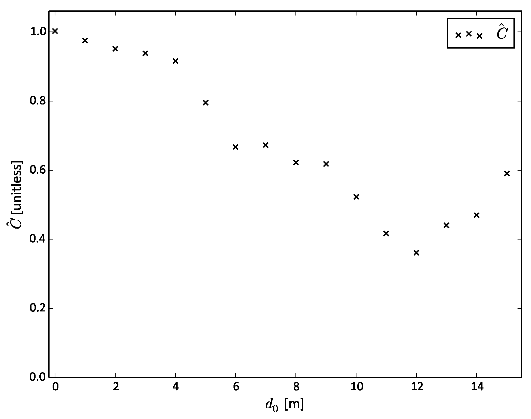
We applied Equation (1) to the experimental FCD described in Section 3.1. Similar to [30], the reference distance $d_0$ was retrieved from the car’s controller area network (CAN) bus, where a sensor recorded the rotation of the car’s drive axle. We set ${\sigma }_x={\sigma }_y=3\mathrm{m}$. This value was chosen according to our experience with the GPS device in the recording environment. The results of Equation (2) imply the following: if the measurement error in the data has a variance of ${\mathit{Var}}_{\mathit{gps}}$ and if it is not affected by autocorrelation, then $\widehat{C}$ is exactly zero. If $\widehat{C}$ is positive there must be autocorrelation in the data.

We found that $\overline{d^m}$ always exceeded the reference distance $d_0$ derived from the CAN bus, such that the average of $d^m-d_0$ equalled around $0.7\mathrm{m}$. Hence, the data confirm that the GPS overestimates distances and allow to calculate $\widehat{C}$. Figure 1 shows the value of $\widehat{C}$ for different reference distances $d_0$ in $1\mathrm{m}$ bins. $\widehat{C}$ is always positive. The measurement error in the experimental FCD is affected by positive autocorrelation. This means that consecutive position estimates have very similar error. The spread of this error is considerably less than suggested by ${\mathit{Var}}_{\mathit{gps}}$. The autocorrelation in Figure 1 decreases with increasing reference distance $d_0$. This indicates that the measurement error in the data is also spatially autocorrelated. Note that Equation (1) provides an estimate of the autocorrelation of GPS measurement error with respect to ${\mathit{Var}}_{\mathit{gps}}$. If we had chosen smaller values for ${\sigma }_x$ and ${\sigma }_y$, for example ${\sigma }_x={\sigma }_y=2\mathrm{m}$, the estimated autocorrelation in Figure 1 would also be smaller. However, $\widehat{C}$ would still be positive and it would still follow the same decreasing trend. This means that we could still conclude that there is temporal and spatial autocorrelation in the data.

Figure 1. The autocorrelation of GPS measurement error in the experimental FCD. The autocorrelation ($\widehat{C}$) decreases as the reference distance ($d_0$) increases. $d_0$ is the distance between recording two consecutive position estimates according to the car’s CAN bus.

Figure 1. The autocorrelation of GPS measurement error in the experimental FCD. The autocorrelation ($\widehat{C}$) decreases as the reference distance ($d_0$) increases. $d_0$ is the distance between recording two consecutive position estimates according to the car’s CAN bus.

The results in Figure 1 are in agreement with empirical findings from the published literature. GPS measurement error is affected by both spatial and temporal autocorrelation [21,22,23]. This autocorrelation can be interpreted as a quality measure for movement data [24]. Although there is measurement error in the FCD, this error is similar for consecutive position estimates. If movement parameters such as distance, direction or speed are calculated from these, the error tends to cancel out. Therefore, we claim that it is legitimate to treat the FCD sampled at $1\mathrm{Hz}$ as an approximation of the true movement of the floating car. On a first glance, this conclusion contradicts with results obtained by other authors. In [45], a Monte Carlo simulation is used to illustrate that measurement error in trajectories sampled at high frequencies does not allow to calculate realistic movement parameters. However, this simulation assumes that GPS measurement error scatters entirely randomly between each two consecutive position estimates. Figure 1 shows that this is not the case for our experimental FCD.

5. Assessing the Influence of Interpolation Error

Interpolation error is closely related to the temporal sampling rate at which movement is recorded: the smaller the time interval between two position estimates, the smaller the interpolation error. In this section we show the influence of interpolation error on movement parameters derived from FCD at different sampling frequencies. We defined four metrics for interpolation error and evaluated these with the experimental FCD described in Section 3.1.

5.1. Rediscretizing the Trajectories

As the true behaviour of a floating car cannot be described with discrete measurements, FCD recorded at different sampling frequencies have to be compared against one another. A similar approach is used in movement ecology to analyse the effects of the sampling rate on simulated random walks [39,40]. We define the experimental FCD recorded at $1\mathrm{Hz}$ to be the reference movement. We showed in Section 4 that the FCD were affected by autocorrelation. Hence, this approximation is legitimate. From the FCD at $1\mathrm{Hz}$ we calculated the reference path (${\mathbf{\Pi }}_{\mathbf{0}}$), the reference distance ($d_0$), the reference speed ($v_0$) and the reference direction (${\theta }_0$) according to Table 1. Then we rediscretized the FCD and re-calculated the movement parameters for larger sampling intervals.

The rediscretization of factor k describes how much the temporal sampling rate is reduced by. For example, a rediscretization of $k=3$ means that the sampling rate is decreased from $1\mathrm{Hz}$ to $1/3\mathrm{Hz}$ (see Figure 2). The use of a moving window during rediscretization ensures that only those elements of the reference and the rediscretized movement are compared that represent the same phases of movement. For a rediscretization of factor k each moving window first partitions the movement into a trajectory segment ${\mathit{\tau }}_{\mathbf{0}}=<({\mathit{P}}_{\mathit{i}},t_i),...,({\mathit{P}}_{\mathit{i}+\mathit{k}},t_{i+k})>$ consisting of $k+1$ spatio-temporal positions. ${\mathit{\tau }}_{\mathbf{0}}$ is then rediscretized to ${\mathit{\tau }}^{\mathit{m}}=<({\mathit{P}}_{\mathit{i}},t_i),({\mathit{P}}_{\mathit{i}+\mathit{k}},t_{i+k})>$ consisting of two spatio-temporal positions, one at the start position of ${\mathit{\tau }}_{\mathbf{0}}$ and the other at the end position. ${\mathit{\tau }}_{\mathbf{0}}$ and ${\mathit{\tau }}^{\mathit{m}}$ represent the same movement at different sampling intervals. They are therefore referred to as a pair of matching movement.

Figure 2. Rediscretizing the FCD. The reference movement at $1\mathrm{Hz}$ is rediscretized to a resolution of $1/3\mathrm{Hz}$, i.e., $k=3$. In a the moving window is at its initial location and encompasses the movement between $({\mathit{P}}_{\mathbf{1}},t_1)$ and $({\mathit{P}}_{\mathbf{4}},t_4)$. The solid red line represents the reference movement, the dashed red line its rediscretization. In b the moving window has shifted forward , so that the reference movement and its rediscretization are now compared between $({\mathit{P}}_{\mathbf{2}},t_2)$ and $({\mathit{P}}_{\mathbf{5}},t_5)$.

Figure 2. Rediscretizing the FCD. The reference movement at $1\mathrm{Hz}$ is rediscretized to a resolution of $1/3\mathrm{Hz}$, i.e., $k=3$. In a the moving window is at its initial location and encompasses the movement between $({\mathit{P}}_{\mathbf{1}},t_1)$ and $({\mathit{P}}_{\mathbf{4}},t_4)$. The solid red line represents the reference movement, the dashed red line its rediscretization. In b the moving window has shifted forward , so that the reference movement and its rediscretization are now compared between $({\mathit{P}}_{\mathbf{2}},t_2)$ and $({\mathit{P}}_{\mathbf{5}},t_5)$.

5.2. Metrics for Interpolation Error

Interpolation error causes the measured path ${\mathbf{\Pi }}^{\mathit{m}}$ to differ from the reference path ${\mathbf{\Pi }}_{\mathbf{0}}$. Henceforth, we refer to this as path uncertainty. Path uncertainty affects not only the geometry of the path (see Figure 3) but also the interpolated distance $d^m$. As $d^m$ follows a straight line between two positions it is always less than or equal to the reference distance $d_0$.

Figure 3. Path uncertainty and its effect on measured distance $d^m$. The measured distance $d^m$ (dashed line) is smaller than the reference distance $d_0$ (solid line). Interpolation error causes a systematic underestimation of distance.

Figure 3. Path uncertainty and its effect on measured distance $d^m$. The measured distance $d^m$ (dashed line) is smaller than the reference distance $d_0$ (solid line). Interpolation error causes a systematic underestimation of distance.

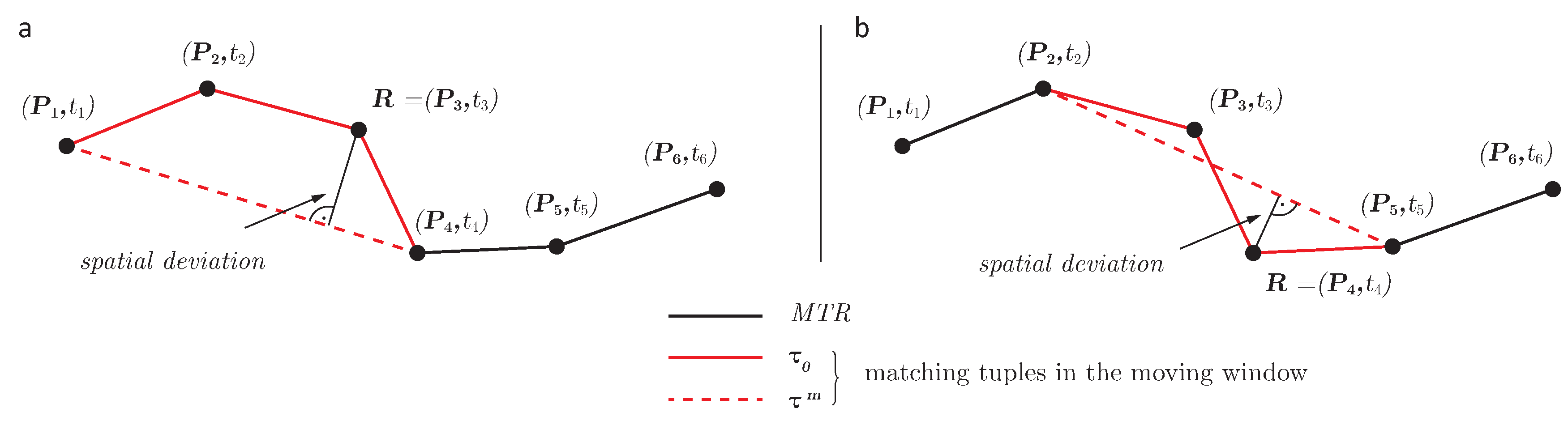
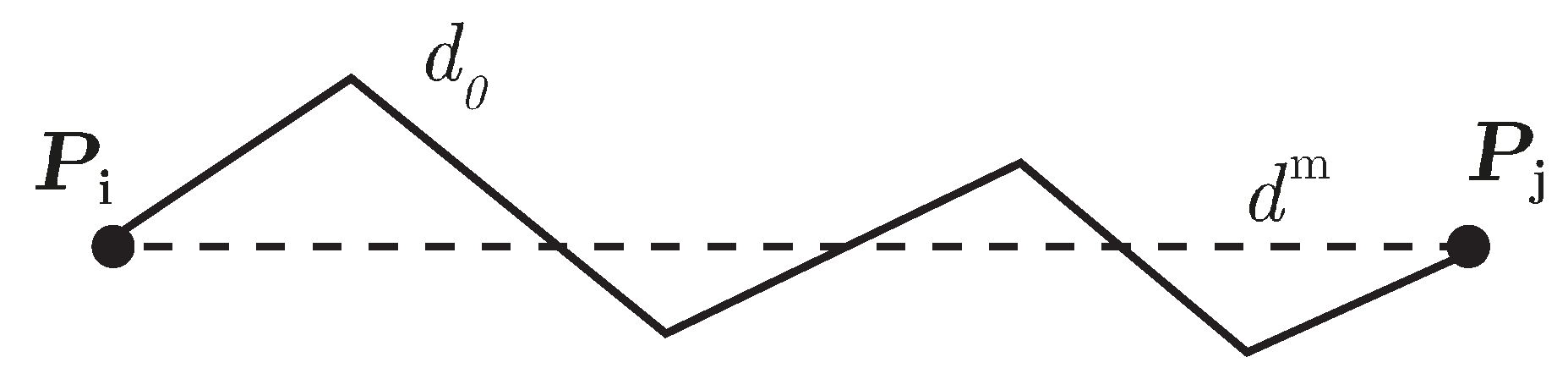
Path uncertainty is a measure of the path difference after rediscretization. For each pair of matching movement we calculated two parameters that allow us to describe the path uncertainty, these being the distance difference and the maximum spatial deviation.

Distance difference, on the one hand, is a metric of how much the length of the rediscretized distance differs from the reference distance:

$$\mathit{\text{Distance}}\mathit{\text{difference}}=d_0-d^m$$

(3)

Spatial deviation, on the other hand, is a metric of how much the spatial location of the rediscretized path differs from that of the reference path. The calculation of the spatial deviation is based on R, the point along ${\mathbf{\Pi }}_{\mathbf{0}}$ that is farthest from ${\mathbf{\Pi }}^{\mathit{m}}$. In Figure 2a, for example, R is at $({\mathit{P}}_{\mathbf{3}},t_3)$. The perpendicular (spatial) distance from R to ${\mathbf{\Pi }}^{\mathit{m}}$ is the spatial deviation. Thus,

$$\mathit{\text{Spatial}}\mathit{\text{deviation}}=D(\mathit{R},{\mathbf{\Pi }}^{\mathit{m}})$$

(4)

As each pair of matching movement has identical first and last positions and both are interpolated linearly, R is bound to be one of the positions along the reference path. Hence, it suffices to calculate the perpendicular distance from the $k-1$ measured positions between start and end point of ${\mathbf{\Pi }}_{\mathbf{0}}$ to ${\mathbf{\Pi }}^{\mathit{m}}$ and to then select the maximum of these.

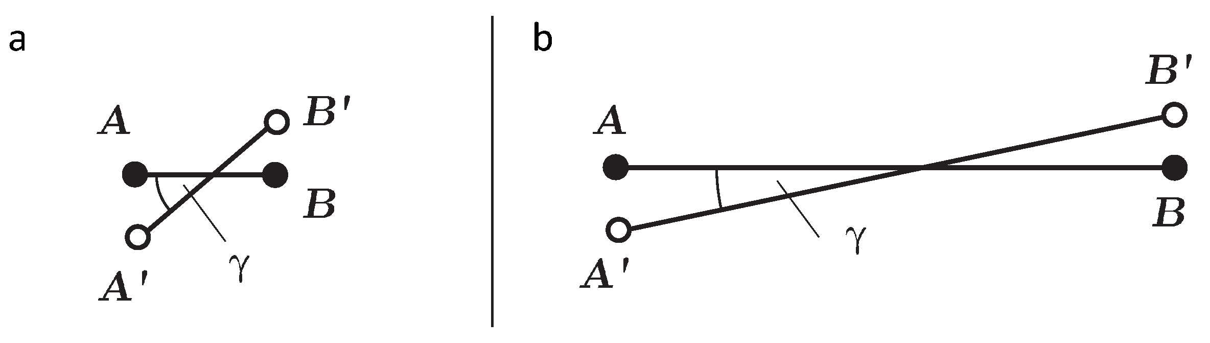
Interpolation error affects speed and direction in two ways: firstly, path uncertainty causes the measured speed and direction to differ from the reference speed and direction. Since $d^m\le d_0$, interpolation error tends to underestimate speed: the object can not have moved more slowly to reach the next known position than $v^m$, but it could have moved more rapidly and taken a longer path.

Secondly, the object’s spatio-temporal progression along the path is uncertain. The measured speed $v^m$ is an average value over the time period between two position estimates. An object moving at a variable speed and another moving at a uniform speed can have the same average speed but only the latter of the two will be captured appropriately by a GPS trajectory.

Henceforth we refer to the uncertainty concerning the spatial path and spatio-temporal progression of an object as dynamic uncertainty. This uncertainty has two aspects. It causes $v^m$ to differ from $v_0$, referred to as speed difference, and ${\theta }^m$ to differ from ${\theta }_0$, referred to as angular deviation.

The speed difference provides a means of assessing information concerning the speed along the reference movement that has been averaged out by interpolation. For a rediscretization of factor k, the measured speed $v^m$ was first calculated between the two positions along ${\mathit{\tau }}^{\mathit{m}}$. Since ${\mathit{\tau }}_{\mathbf{0}}$ consists of $k+1$ positions there are k reference speed measurements between these. Consequently, $v_0\left(i\right)$ is the reference speed between the $i^{\mathit{th}}$ and $i+1^{\mathit{th}}$ consecutive positions along ${\mathit{\tau }}^{\mathit{m}}$, where $i\in \{1,...,k\}$. Then, we retrieved the difference between each $v_0\left(i\right)$ and $v^m$. Hence, speed difference is defined as

$$\mathit{\text{Speed}}\mathit{\text{difference}}=|v_0\left(i\right)-v^m|$$

(5)

The angular deviation, on the other hand, describes the absolute difference between the direction of ${\mathit{\tau }}^{\mathit{m}}$ as compared to the direction of ${\mathit{\tau }}_{\mathbf{0}}$. As we did with the speed difference, we first calculated the direction ${\theta }^m$ between the two positions along ${\mathit{\tau }}^{\mathit{m}}$. Then, we calculated the direction ${\theta }_0\left(i\right)$ between the $i^{\mathit{th}}$ and the $i+1^{\mathit{th}}$ position along ${\mathit{\tau }}_{\mathbf{0}}$, where $i\in \{1,...,k\}$. Finally, we determined the absolute difference between each ${\theta }_0\left(i\right)$ and ${\theta }^m$. Hence, angular deviation is defined as

$$\mathit{\text{Angular}}\mathit{\text{deviation}}=|{\theta }_0\left(i\right)-{\theta }^m|$$

(6)

5.3. Evaluation of Interpolation Error in Real-World FCD

In this subsection we evaluate the effects of interpolation error on movement parameters derived from FCD at different sampling frequencies. We used the data set described in Section 3.1.

Starting from the FCD at $1\mathrm{Hz}$ we performed 19 independent rediscretization steps of factor $k\in \{2,...,20\}$. For each rediscretization step we searched the trajectory data for all possible pairs of matching movement. We then calculated movement parameters and evaluated the four metrics for interpolation error. In the following paragraph we present our findings and interpret them with respect to well-known results from RW theory.

Figure 4 shows the distance difference after rediscretization. The distance difference is always positive; compared to $d_0$, trajectories sampled at lower sampling frequencies cause an underestimation of distance. The median, inter-quartile ranges and whiskers increase in an almost quadratic fashion. With less frequent sampling some of the $d^m$ become very small, whereas others remain almost unchanged.

Figure 4. Distance difference after a rediscretization of factor k. In (a), the box-plot has whiskers at the $99\%$ quantile; in (b) it has no whiskers.

Figure 4. Distance difference after a rediscretization of factor k. In (a), the box-plot has whiskers at the $99\%$ quantile; in (b) it has no whiskers.

Similar results have also been previously explained and explored in velocity jump simulations of correlated random walks [39,40]. In a velocity jump process, an object moves with a fixed speed for a random time interval and then turns to a new direction, usually one drawn from a circular normal distribution; the iteration of these steps creates a correlated random walk. In [39,40] the authors rediscretized these random walks using decreasing sampling frequencies and recorded the change in speed after rediscretization. They found that the negative natural logarithm of mean observed speed increases in a linear manner with decreasing sampling rate. These findings can easily be related to distance: since the velocity jump process assumes true speed to be constant, any change in observed speed is caused by a change in the observed distance. These results therefore suggest a decay in the observed distance and an increase in its variability. Our results also indicate an increasing distance difference with decreasing sampling rate, as well as an increase in the variability of distance difference (see the interquartile range and the whiskers in Figure 4).

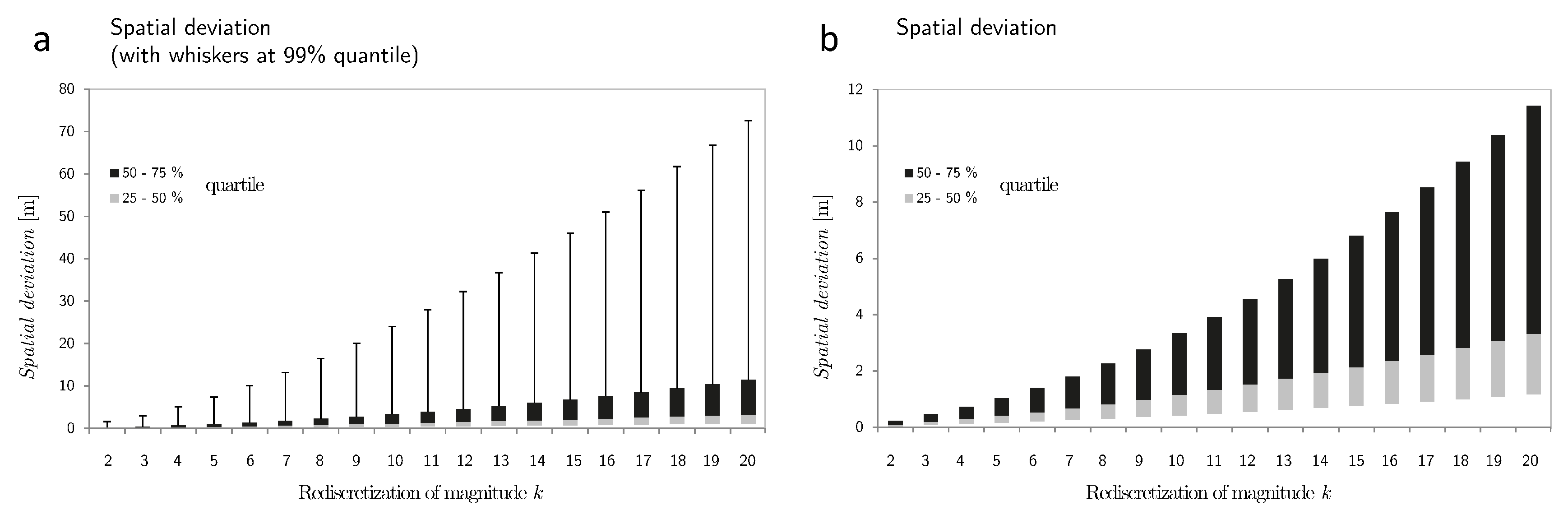
Figure 5 shows the spatial deviation after rediscretization. With decreasing sampling frequencies the spatial deviation increases quadratically. Again, this finding relates to random walk theory, where the mean squared displacement ($\mathit{\text{MSD}}$) is used to describe the mean spatial extent of a random motion. In a random walk, the $\mathit{\text{MSD}}$ increases as the sampling rate decreases [36,37].

Figure 5. Spatial deviation after a rediscretization of factor k. In (a), the box-plot has whiskers at the $99\%$ quantile; in (b) it has no whiskers.

Figure 5. Spatial deviation after a rediscretization of factor k. In (a), the box-plot has whiskers at the $99\%$ quantile; in (b) it has no whiskers.

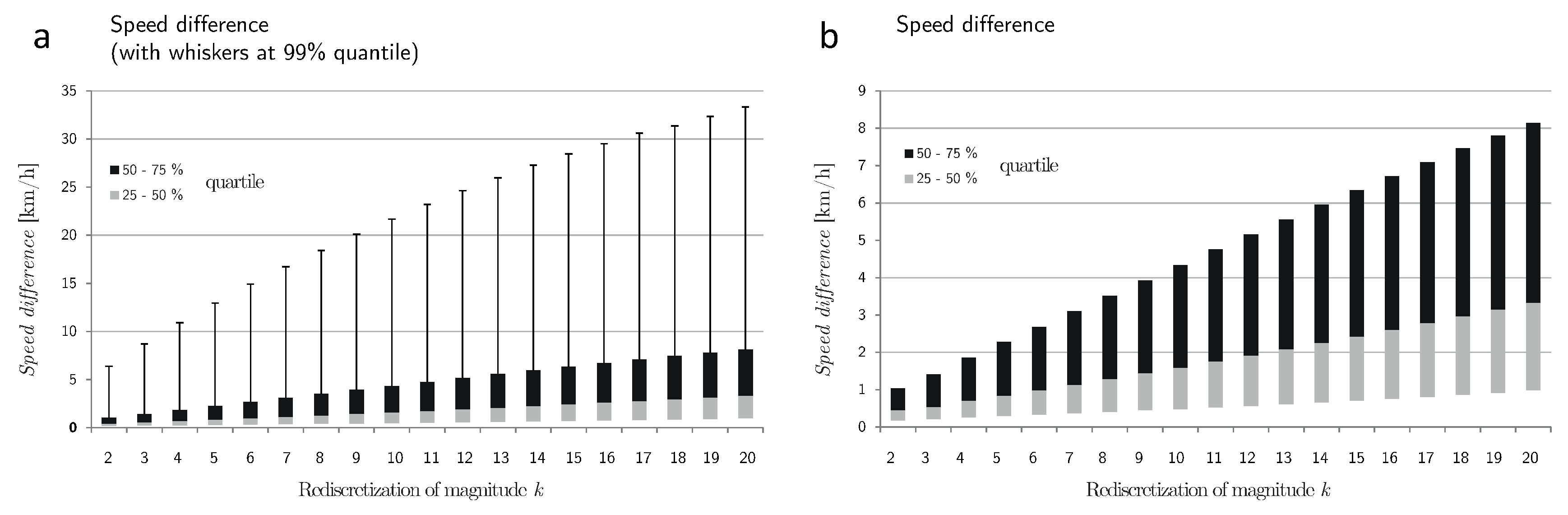
Figure 6 shows the speed difference after rediscretization. In contrast to path uncertainty, speed difference increases in an approximately logarithmic fashion. This means that the information loss caused by a decrease from high to medium sampling frequencies (e.g., from $k=2$ to $k=5$) is considerably greater than the loss caused by a decrease from medium to low sampling frequencies (e.g., from $k=10$ to $k=15$). This holds true for the median, the quartiles and the whiskers. Similarly, Figure 7 illustrates the speed difference between matching sequences along a real-world GPS trajectory for a redicretization of $k\in \{2,3,5,10\}$.

The findings in Figure 6 are in agreement with the results obtained in [39,40], where the change of observed speed in a simulation was found to be exponential. Nonetheless, there is a fundamental difference: the change in speed reported by these authors was due to a change of observed distance in a rediscretized velocity jump process of constant speed. This corresponds to the distance difference in Figure 5. In contrast, the speed difference in Figure 7 is due to a change in the observed distance and to an incorrect perception of the dynamics of movement. The observed speed difference is therefore much greater than the distance difference in Figure 4.

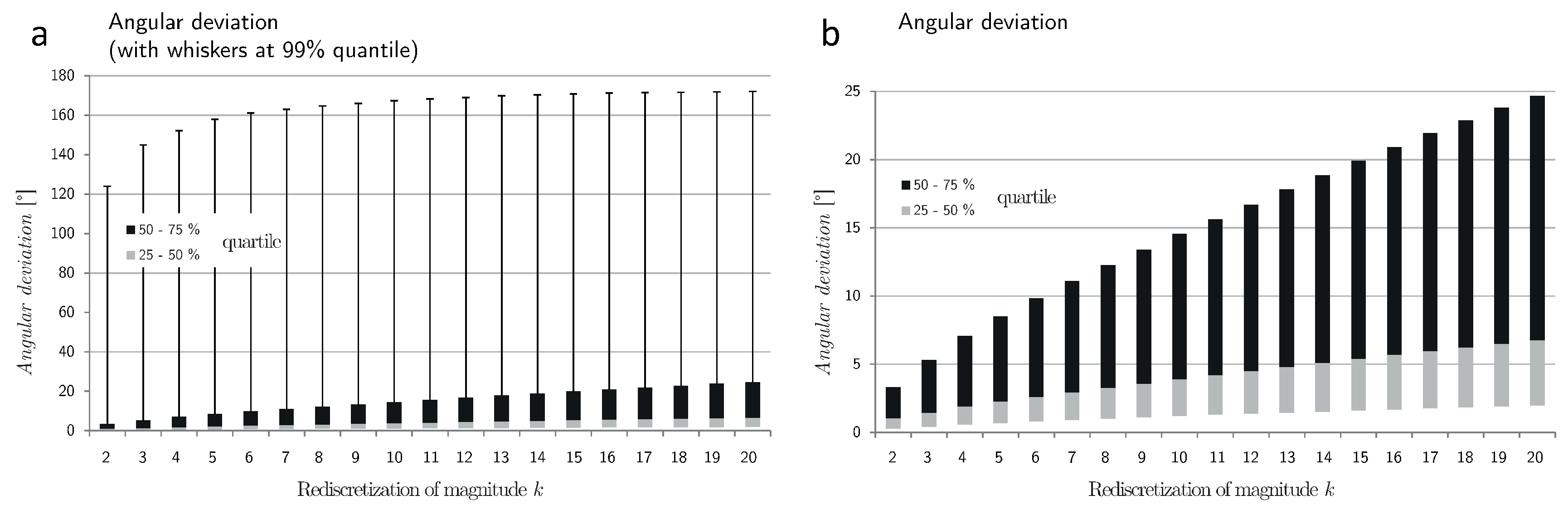
Figure 8 shows the angular deviation after rediscretization. As was the case with speed difference, angular deviation increases in an approximately logarithmic manner. Up to $k=20$ the median of the angular deviation remains well below ${10}^{\circ }$. However, for even a very moderate increase of the sampling rate to $k=2$ the upper quartile already shows considerable deviation of ${120}^{\circ }$. Again, the results in Figure 8 are in good agreement with results from simulations where angular deviation was found to change logarithmically with decreasing sampling rate [40].

Figure 6. Speed difference after a rediscretization of factor k. In (a), the box-plot has whiskers at the $99\%$ quantile; in (b) it has no whiskers.

Figure 6. Speed difference after a rediscretization of factor k. In (a), the box-plot has whiskers at the $99\%$ quantile; in (b) it has no whiskers.

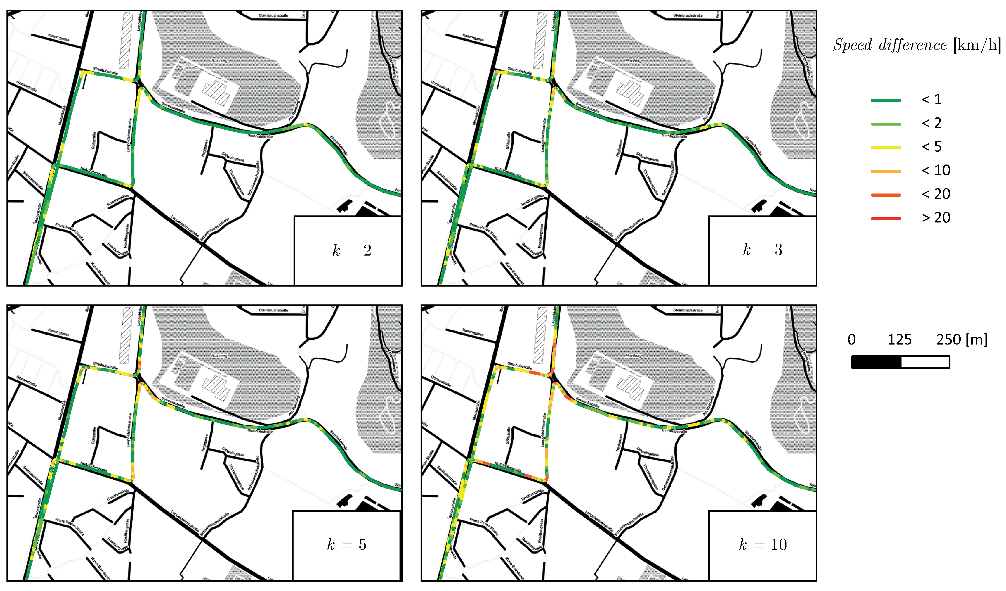
Figure 7. Speed difference for a rediscretization of factor k mapped to the FCD recorded at $1\mathrm{Hz}$. The green color indicates a low speed difference ($<1\mathrm{km}/\mathrm{h}$), the red color a high speed difference ($>20\mathrm{km}/\mathrm{h}$). A slightly lower sampling rate ($k=5$) already results in a severe loss of information; green and red phases alternate frequently. Especially near to road intersections where the car is decelerating or accelerating speed differs by up to $20\mathrm{km}/\mathrm{h}$ from the reference.

Figure 7. Speed difference for a rediscretization of factor k mapped to the FCD recorded at $1\mathrm{Hz}$. The green color indicates a low speed difference ($<1\mathrm{km}/\mathrm{h}$), the red color a high speed difference ($>20\mathrm{km}/\mathrm{h}$). A slightly lower sampling rate ($k=5$) already results in a severe loss of information; green and red phases alternate frequently. Especially near to road intersections where the car is decelerating or accelerating speed differs by up to $20\mathrm{km}/\mathrm{h}$ from the reference.

Figure 8. Angular deviation after a rediscretization of factor k. In (a), the box-plot has whiskers at the $99\%$ quantile; in (b) it has no whiskers.

Figure 8. Angular deviation after a rediscretization of factor k. In (a), the box-plot has whiskers at the $99\%$ quantile; in (b) it has no whiskers.

6. Temporal Sampling Recommendations for Recording FCD with a GPS

In this paper we discussed and evaluated the influence of error on movement parameters calculated from FCD recorded with a GPS. First, we showed that measurement error in the experimental FCD was highly autocorrelated. This built the basis for all consecutive analyses. Then we defined four metrics for assessing the influence of interpolation error and evaluated them in the experimental FCD. In this section we summarized our results and draw our conclusions, which we then used to give temporal sampling recommendations for recording FCD with a GPS. These recommendations aim at preserving the true characteristics of the movement parameters and minimizing the influence of errors, while at the same time avoiding the collection of redundant information. A synthesis of the sampling recommendations can be found in Table 2.

Table 2. Temporal sampling recommendations for recording FCD with a GPS. The rationale behind all values is explained in detail in the text.

Movement Parameter		Sampling Rate [Hz]
Spatial Path	Π	1/3–1/5
Distance	d	1/5–1/10
Speed	v	1–1/2
Direction	θ	1/3–1/5

Table 2. Temporal sampling recommendations for recording FCD with a GPS. The rationale behind all values is explained in detail in the text.

Movement Parameter		Sampling Rate [Hz]
Spatial Path	Π	1/3–1/5
Distance	d	1/5–1/10
Speed	v	1–1/2
Direction	θ	1/3–1/5

6.1. Path

Interpolation error causes a spatial deviation of ${\mathbf{\Pi }}^{\mathit{m}}$ from ${\mathbf{\Pi }}_{\mathbf{0}}$. In the experimental FCD, spatial deviation is still small after a moderate rediscretization (see Figure 5). We therefore propose a sampling rate between $1/3$ to $1/5\mathrm{Hz}$ for recording paths in order to avoid recording redundant information. For this sampling rate the median spatial deviation is still well below $1\mathrm{m}$.

6.2. (Cumulative) Distance

GPS measurement error causes a systematic overestimation of distances, whereas interpolation error causes a systematic underestimation of distances. An appropriate temporal sampling rate therefore has to find a balance between these two contradictory influences. From our empirical data we observed that, on average, this balance occurs at a sampling rate of about $1/8\mathrm{Hz}$. For this sampling rate the mean overestimation of distance caused by measurement error equals roughly $0.7$ meter (see Section 4), and so does the mean distance difference caused by interpolation error (see Figure 4). This observation is based on experimental data and should therefore only be treated as a rough approximation. Hence, we propose a sampling rate between $1/5$ and $1/10\mathrm{Hz}$ for recording distances by means of FCD. The upper limit of $1/5\mathrm{Hz}$ tends towards an overestimation of distance while the lower limit of $1/10\mathrm{Hz}$ tends towards an underestimation.

6.3. Speed

Due to the autocorrelation of measurement error high sampling frequencies tend to have positive effects on the calculation of distances and speed. The influence of measurement error tends to cancel out for speed that is derived from two position estimates that are close together in space and time. However, high sampling frequencies also result in a systematic overestimation of distance and, therefore, also of speed. In contrast to distance, speed is not cumulative and, therefore, these slight systematic errors are not cumulative.

For interpolation error, our experiments show that speed difference already increases significantly for a small rediscretization (see Figure 7) causing the interpolated speed $v^m$ to differ significantly from $v_0$. Since both measurement and interpolation errors suggest that very frequent sampling is required we propose a sampling rate of at least 1 to $1/2\mathrm{Hz}$ for recording speed and acceleration from FCD.

6.4. Direction

Due to spatio-temporal autocorrelation of measurement error high sampling frequencies also tend to have positive effects on the calculation of direction. However, if two uncertain positions are farther apart from each other the direction between these is generally less affected by error. This is visualized in Figure 9, where A and B are two positions in space and ${\mathit{A}}^{\mathbf{\prime }}$ and ${\mathit{B}}^{\mathbf{\prime }}$ are GPS position estimates affected by measurement error.

Figure 9. The influence of measurement error on the direction between two uncertain positions. The angle γ is the difference between the vectors $\mathit{A}\mathit{B}$ and ${\mathit{A}}^{\mathbf{\prime }}{\mathit{B}}^{\mathbf{\prime }}$. In (a), A and B are close together; in (b), they are farther apart. The relative position of ${\mathit{A}}^{\mathbf{\prime }}$ to A and ${\mathit{B}}^{\mathbf{\prime }}$ to B does not change. Still γ in (b) is smaller than in (a).

Figure 9. The influence of measurement error on the direction between two uncertain positions. The angle γ is the difference between the vectors $\mathit{A}\mathit{B}$ and ${\mathit{A}}^{\mathbf{\prime }}{\mathit{B}}^{\mathbf{\prime }}$. In (a), A and B are close together; in (b), they are farther apart. The relative position of ${\mathit{A}}^{\mathbf{\prime }}$ to A and ${\mathit{B}}^{\mathbf{\prime }}$ to B does not change. Still γ in (b) is smaller than in (a).

The effects of interpolation error on angular deviation are illustrated in Figure 8. For three quartiles the angular deviation is moderate up to around $1/5\mathrm{Hz}$ while for the remaining upper quartile the angular deviation is very high for all sampling frequencies. We propose a sampling rate of around $1/3$ to $1/5\mathrm{Hz}$ for recording directions and turning angles.

Table 2 summarizes our findings and presents temporal sampling recommendations for recording FCD with a GPS. The strategy aims to reduce the influence of measurement and interpolation errors when calculating movement parameters between two consecutive GPS position estimates. Similar approaches have previously been used in the published literature to address complementary aspects of movement data sampling. Filtering techniques were shown to reduce GPS error [30]. The effects of sampling rate on movement parameters were described in synthetic random walk data [39,40].

7. Dicussion

Our approach differs from those adopted by previous authors: firstly, we have concentrated on the temporal sampling rate as the only regulatory instrument for controlling the quality of information in trajectory data. Filtering, for example, is not addressed in our research as it has already received considerable attention from other authors [29,30]. Secondly, our movement parameters have been derived from real-world movement data rather than generated in a simulation. Real-world data are affected by measurement and interpolation error and these have sometimes contradicting influence on the calculation of movement parameters [15]. In this research we addressed both types of error, aiming to find a balanced strategy to reduce them. Naturally, the characteristics of the data influence our findings. The FCD were recorded in Salzburg, a city with many narrow and angled streets. The floating cars often change speed and turn frequently. Thus, interpolation error is expected to be higher than in a road network consisting of long straights where cars move uniformly.

It may sometimes not be possible to use the sampling frequencies recommended in this paper to record FCD. We therefore discuss ways of how to interpret useful results from sparsely sampled data. Firstly, some movement parameters are not affected by the sampling rate. The sinuosity index is a measure of how target-oriented movement is [36] and it is not affected by the sampling rate. Secondly, the FCD can be enhanced with additional geographical information. Rather than moving freely in space, floating cars are confined to a road network. Geometric and attributive information of the network can be useful for reconstructing the movement of the car. The distance along a road network might, for example, allow an accurate estimate to be made of a vehicle’s travelled distance where the data is sparsely sampled. Thirdly, probabilistic models such as the Brownian bridge movement model [34] can be used to describe the probable movement of an object rather than a crisp line as defined by linear interpolation. In a road network the probable movement is the set of all paths that allow a vehicle to reach the next measured position along the trajectory within the available time [27]. However, even for FCD that were recorded at sparser sampling frequencies our findings can be instructive. They reveal the error that was most likely introduced when collecting the FCD.

Euclidean Space or Network Space?

In this article all movement parameters were calculated in two-dimensional Euclidean space. However, floating cars move in a road network. For many practical applications it is necessary to first map-match the FCD to network space. In network space the current position of the floating car can be expressed as a combination of the link ID and the relative position on the link [46]. In this section we discuss the influence of the sampling rate on map-matching and movement parameters in network space. We focus on the following two aspects:

• How can our findings support map-matching from two-dimensional space to network space?
• Which movement parameters should rather be calculated from the trajectory in two-dimensional Euclidean space and which in network space?

(1) Since floating car data are affected by error, they cannot be simply projected to network space. Due to measurement error, position estimates are likely to lie off the roads. Moreover, due to interpolation error, it might not be possible to find a unique path between two correctly map-matched position estimates. Hence, a map-matching algorithm is needed to associate the GPS trajectory to the road network. There are four types of map-matching algorithms [47]. Geometric algorithms use geometric properties of the trajectory and the road network. Topological algorithms also consider the connectivity and topology of the road network. Probabilistic algorithms create an error region around each GPS position estimates in order to single out candidate links in the road network, where the car might have travelled. From these candidates the algorithm picks the most probable. Advanced map-matching algorithms use advanced statistical concepts to link the trajectory to the road network.

Most map-matching algorithms require reliable movement parameters to associates a trajectory to a road network. These movement parameters inevitably have to be calculated in two-dimensional Euclidean space. Simple geometric algorithms only consider the path and its shape [48,49]. Other, more sophisticated algorithms compare the direction of the trajectory to the direction of the links in the road network [50]. Yet other algorithms use information on the distance travelled [51] or the speed of the floating car [52]. Our findings can help to choose an appropriate map-matching algorithm for a given sampling rate. We showed that for trajectories sampled at $1\mathrm{Hz}$ the direction tends to be unstable and distances tend to be overestimated; for trajectories sampled at $1/5\mathrm{Hz}$ average speed fails to reflect the actual speed of the car; for trajectories sampled at $1/20\mathrm{Hz}$ the recorded path already differs considerably from the actual path. These examples show that FCD require different map-matching approaches depending on the sampling rate at which they were recorded.

For FCD recorded at very low sampling rates ($<1/20\mathrm{Hz}$) traditional map-matching algorithms are likely to provide poor results. Thus, special algorithms for low-frequency FCD have to be used [46,53]. These algorithms connect position estimates with candidate routes; the trajectory is matched to the most probable of these routes. However, also the accuracy of these algorithms decreases with the sampling rate [54]. At lower sampling rates there are many possible paths between two consecutive position estimates and map-matching is more likely to choose an incorrect link [28].

(2) Finally, we discuss, which data are more suitable for calculating movement parameters, the raw GPS trajectory data in two-dimensional space or the map-matched trajectory data in network space. In two-dimensional space, a trajectory will be longer than it really was if sampling is too frequent. It will be shorter, if sampling is too sparse. In order to avoid a systematic error in either direction, it is preferable to first map-match the FCD and to derive distances in network space. Similar arguments can be made for path and direction. The road network defines the path and the direction of a floating car. Therefore, it is more reasonable to deduce both from the map-matched trajectory. However, if average speed is derived from network space the projection from two-dimensional space might dislocate two positions, which makes speed occasionally faster or slower than it really was. As GPS trajectories are affected by strong spatio-temporal autocorrelation, speed calculations between two consecutive position estimates should be very accurate. Hence, it is preferable to calculate average speed in two-dimensional Euclidean space.