An Extended Semi-Supervised Regression Approach with Co-Training and Geographical Weighted Regression: A Case Study of Housing Prices in Beijing

Abstract

This paper proposes an extended semi-supervised regression approach to enhance the prediction accuracy of housing prices within the geographical information science field. The method, referred to as co-training geographical weighted regression (COGWR), aims to fully utilize the positive aspects of both the geographical weighted regression (GWR) method and the semi-supervised learning paradigm. Housing prices in Beijing are assessed to validate the feasibility of the proposed model. The COGWR model demonstrated a better goodness-of-fit than the GWR when housing price data were limited because a COGWR is able to effectively absorb no-price data with explanatory variables into its learning by considering spatial variations and nonstationarity that may introduce significant biases into housing prices. This result demonstrates that a semisupervised geographic weighted regression may be effectively used to predict housing prices.

1. Introduction

The housing market is defined as one where housing services are allocated by the mechanism of supply and demand and could be influenced by macro-economic variables, spatial differences, characteristics of the community structure and environmental amenities [1,2]. Changing housing prices have been of concern to both residents and governments in that they influence the socio-economic conditions and have a further impact on the national economic stability [2]. Therefore, the issue of predicting housing prices has recently been a focus of research in the geo-information field [3,4,5,6].

Housing prices are typically predicted via the establishment of a regression model that uses house price parameters (e.g., structural and neighborhood characteristics of the real estate) [7,8]. Many authors have focused on the hedonic model to predict housing prices, and different hedonic models are compared in real estate economics [9,10,11]. Although hedonic regression models are widely adopted, the presence of spatial dependence is detrimental to the efficiency and unbiasedness of the OLS model in traditional hedonic models. Spatial location is an important factor in housing prices [10]. Real estate prices tend to be spatially heterogeneous [12]. Therefore, spatial economics models have been proposed to address these issues. LeSage and Pace provide a broad review of these methods [13,14]. Goodman and Thibodeau introduce the concept of hierarchical linear modeling in which dwelling characteristics, neighborhood characteristics and submarkets interact to influence housing prices [15]. Brunsdon and Fotheringham propose a geographically-weighted regression as a local variation modeling technique to explore spatial nonstationarity [6,7].

Supposing that the number of house samples is limited, researchers have yet to determine how to enhance the goodness-of-fit of housing prices by using explanatory variables for houses where the price is unknown. Semi-supervised learning is an efficient approach that attempts to integrate no-price data to achieve a strong generalization by using multiple learners, and some studies have utilized semi-supervised regression models to address this issue [16,17,18,19,20]. However, when traditional semi-supervised regression methods are applied to spatial data, the processes are assumed to be constant over space, which is not accurate. For housing price data, the assumption of stability over space is generally unrealistic, as housing price parameters tend to vary over a study area [21].

In recognizing the above challenges, this research proposes an extended semi-supervised regression approach to fully utilize the advantages of both the geographical weighted regression and the semi-supervised learning methods to increase the goodness-of-fit with respect to housing price data.

The remainder of this paper is organized as follows. In Section 2, related studies are briefly reviewed. In Section 3, the experimental data and proposed approach are introduced. Section 4 describes the experimental results. Section 5 provides concluding remarks.

2. Literature Review

The term hedonic is used to describe “the weighting of the relative importance of various components among others in constructing an index of usefulness and desirability” [22]. The hedonic price model is based on the hedonic hypothesis that goods are valued for their utility-bearing attributes or characteristics [23]. If the prices of these attributes are known, or can be estimated, and the attribute composition of a particular differentiated good is also known, the hedonic methodology will provide a framework for value estimation [24]. The hedonic model regards houses as a composite commodity formed by structural attributes (age of house, number of bedrooms, presence of a garage, etc.), by locational attributes that vary between properties (good transport links, accessibility to shops and services, proximity to downtown, etc.) and by neighborhood attributes (population density, unemployment, measures of social stress, etc.). The price of a property is assumed to be a realization of the values of these attributes [25].

The conditional parametric model termed geographical weighted regression (GWR) is an explicitly local model and circumvents the problems discussed in the context of discrete modeling of heterogeneity and polynomial regression [6,7]. GWR implicitly assumes continuously-changing price functions and models. A strong advantage of GWR is its flexibility, and the price function needs no prior assumption concerning the price determination process and its spatial variation [26,27]. Lu, B. et al. investigates the GWR model by applying it with alternative, non-Euclidean distance (non-ED) metrics. A case study of a London house price dataset is coupled with hedonic independent variables, where GWR models are calibrated with Euclidean distance (ED), road network distance and travel time metrics. The results indicate that GWR calibrated with a non-Euclidean metric can not only improve the model fit, but also provide additional and useful insights into the nature of varying relationships within the house price dataset [4]. A geographically- and temporally-weighted autoregressive model (GTWAR) has been developed to account for both nonstationary and auto-correlated effects simultaneously and formulates a two-stage least squares framework to estimate this model [5].

However, the GWR model assumes that all explanatory variables vary over space, and the global effects are often neglected; the mixed geographically-weighted regression (MGWR) model has been proposed to explore spatially-stationary and non-stationary effects. It is shown by the MGWR empirical examples that significant spatial variation in some of the estimated parameters is present, while the global effects provide evidence for policy-based linkages and an economically-connected housing market [28]

Considerable interest has been devoted to the non-conventional methods in real estate property assessment. The most commonly-studied methods are neural network-based approaches. The appeal of neural network-based methods lies in that they do not depend on assumptions about the data [29]. Neural networks are more robust to model misspecification and especially to various peculiarities in how various explanatory variables are measured [30]. A fuzzy logic framework has also been proposed as an alternative to conventional property assessment approaches [29,31]. Kuşan, H. et al. introduce household-level data into hedonic models in order to measure the heterogeneity of implicit prices regarding household type, age, educational attainment and income [32].

In the field of semi-supervised learning, labeled identifies the training examples known in advance and unlabeled identifies the training examples that are unknown. In this paper, “labeled data” refers to the sample of known housing prices, and “unlabeled data” refers to the explanatory variables of houses for which prices are unknown. Brefeld et al. developed a co-regularized least squares regression (coRLSR) algorithm to handle larger sets of unlabeled examples based on the co-learning framework, and the experiments show a significant error reduction and large runtime improvement for the semi-parametric approximation [17]. Zhou and Li applied the co-training mechanism to a KNN regression. Two different KNN regression models have been utilized; each model labels unlabeled data for the other regressor, particularly where the labeling confidence is predicted based on the influence of labeling unlabeled samples on the labeled data [18,19].

3. Data and Methods

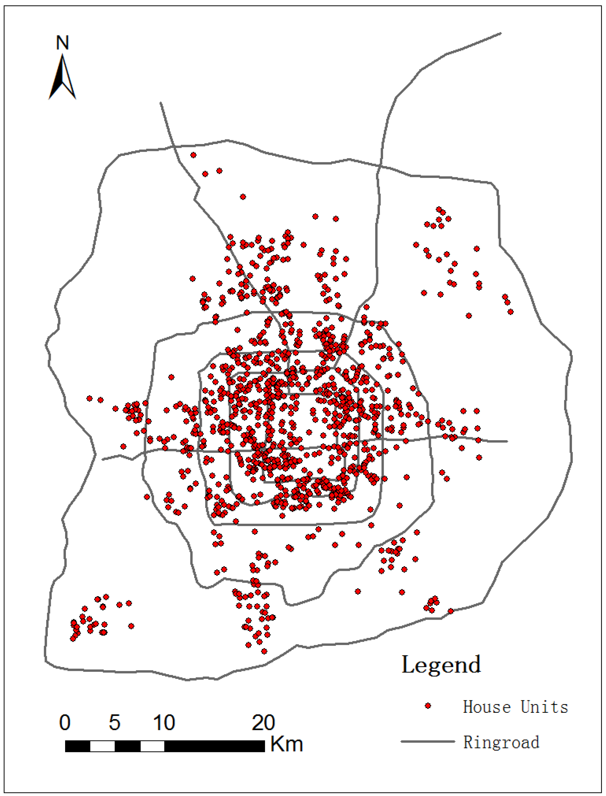
3.1. Data Used in the Experiments

A case study is carried out using housing price data observed in Beijing, China. Beijing is one of the most developed cities and is an economic center in China, with tertiary industries accounting for 71.3% of its GDP. This makes it the first post-industrial city in mainland China. Along with a reform process, both economic prosperity and rapid urbanization have boosted demand for housing in the city. The increased demand for housing was accompanied by increased supply as prices and rents increased [33].

An overview of the housing prices variables is shown in Table 1. A total of 1350 residential houses are included in the study, and their geolocations are shown in Figure 1. The study data are provided by the National Bureau of Statistics, and structural, neighborhood and temporal variables are extracted to explain the house prices in this study.

The dependent variable (lnp) is the logarithmically-transformed sales price of the house, with the price unit of RMB. The structural characteristics of each house are described by five covariates. Total floor area of the house, with the area unit of m², is logarithmically transformed as lnarea_total. The number of bath rooms is expressed as nbath. The management fee of the property, with the fee unit of RMB/m², is logarithmically transformed as lnpfee. The ratio of houses is logarithmically transformed as lnplotratio. Additionally, the green ratio is logarithmically transformed as lngratio. The neighborhood of each house is described by the urban street network of Beijing, which defines the city’s structural skeleton and directly affects the city’s transportation and economic performance. The temporal variable is the age of building at time of sale (age).

Table 1. Variables used to predict housing prices in Beijing, China.

Abbreviation	Description	Minimum	Mean	Maximum
lnp	Log sales transactions price of the house	12.468	14.897	17.990
Structural covariates
lnarea_total	Log of total floor area	2.303	4.317	6.385
nbath	Number of bath rooms	0	1	3
lnpfee	Log fee of property management	−1.513	0.470	6.534
lnplotratio	Log plot ratio of houses	−1.323	0.693	3.401
lngratio	Log green ratio	−4.605	3.401	4.443
Temporal covariates
age	Age of building at time of sale (1996–2015)	1	9	20
Neighborhood covariates
ringroad	Within the major road ring	2	4	6

Table 1. Variables used to predict housing prices in Beijing, China.

Abbreviation	Description	Minimum	Mean	Maximum
lnp	Log sales transactions price of the house	12.468	14.897	17.990
Structural covariates
lnarea_total	Log of total floor area	2.303	4.317	6.385
nbath	Number of bath rooms	0	1	3
lnpfee	Log fee of property management	−1.513	0.470	6.534
lnplotratio	Log plot ratio of houses	−1.323	0.693	3.401
lngratio	Log green ratio	−4.605	3.401	4.443
Temporal covariates
age	Age of building at time of sale (1996–2015)	1	9	20
Neighborhood covariates
ringroad	Within the major road ring	2	4	6

Figure 1. Map of the study area.

Figure 1. Map of the study area.

3.2. Methods

3.2.1. Geographically-Weighted Regression Model

GWR is a non-stationary technique that models the spatially-varying relationships between independent and dependent variables [3,4,5,34]. The GWR model can be expressed as:

$$y_i={\beta }_0\left(u_i,v_i\right)+{\displaystyle \sum }_{k=1}^p{\beta }_k\left(u_i,v_i\right)x_{ik}+{\epsilon }_i i=1,2,\cdots ,n$$

(1)

where the coordinate of point $i$ in space is expressed as $\left(u_i,v_i\right)$; ${\beta }_0\left(u_i,v_i\right)$ represents the intercept value; and ${\beta }_k\left(u_i,v_i\right)$ represents a set of values for the number $p$ of parameters at point $i$. The random error, which conforms to a normal distribution, is denoted as ${\epsilon }_i$, ${\epsilon }_i\sim N\left(0,{\sigma }^2\right)$. There is no correlation in random error between different points: $\text{Cov}\left({\epsilon }_i,{\epsilon }_j\right)=0\left(i\ne j\right)$. The regression parameter ${\widehat{\beta }}_i$ at point $i$ can be attained using the least squares model.

$${\widehat{\beta }}_i={\left(X^{\prime }{W}_{i}X\right)}^{-1}{X}^{\prime }{W}_{i}y$$

(2)

The fitted value $\widehat{y}$ is:

$$\widehat{y}=\left[\begin{array}{c}{\widehat{y}}_1\\ {\widehat{y}}_2\\ \cdots \\ {\widehat{y}}_n\end{array}\right]=\left[\begin{array}{c}{X}_1{\left(X^{\prime }{W}_{1}X\right)}^{-1}{X}^{\prime }{W}_1\\ X_2{\left(X^{\prime }{W}_{2}X\right)}^{-1}{X}^{\prime }{W}_2\\ \cdots \\ X_n{\left(X^{\prime }{W}_{n}X\right)}^{-1}{X}^{\prime }{W}_n\end{array}\right]y$$

(3)

where the weighting matrix $W_i$ is based on the distances between regression point i and the data points around it. Two types of weighting matrix are used, fixed and adaptive kernels. In a fixed kernel function, an optimum spatial kernel bandwidth is calculated and applied over the study area. The most commonly-used fixed weighting function is the Gaussian function:

$$W_{ij}=\text{exp}\left(-\frac{d_{ij}^2}{h^2}\right)$$

(4)

where $h$ is a nonnegative parameter known as bandwidth and produces a decay of influence with the distance between locations i and j.

The commonly-used adaptive weighting is the bi-square function, which represents different bandwidths at location i.

$$W_{ij}=\{\begin{array}{c}{\left[1-{\left(\frac{d_{ij}}{h}\right)}^2\right]}^2, \mathrm{if} d_{ij}<h\\ 0, \mathrm{otherwise}\end{array}$$

(5)

If the predicted value of $y_i$ from GWR is denoted by ${\widehat{y}}_i\left(h\right)$, the sum of the squared error can be written as:

$$\text{CV}\left(h\right)={\displaystyle \sum }_i{\left(y_i-{\widehat{y}}_{\ne i}\left(h\right)\right)}^2$$

(6)

The bandwidth is achieved automatically with an optimization technique by minimizing Equation (6) in terms of goodness-of-fit statistics.

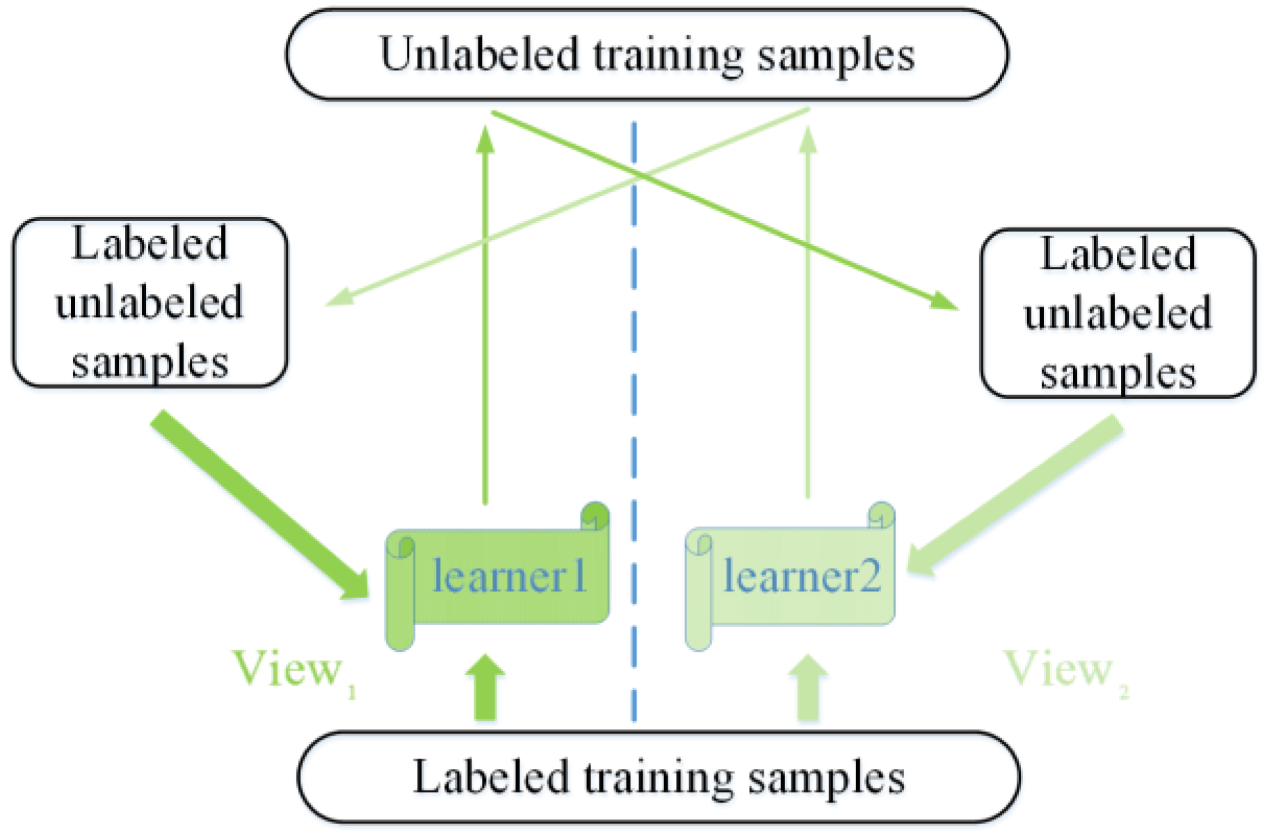
3.2.2. Co-Training Learning Paradigm

The co-training paradigm is one of the most prominent semi-supervised approaches. It was first proposed by Blum and Mitchell, trains two classifiers separately on two different views, e.g., two independent sets of attributes, and uses the prediction of each classifier on unlabeled examples to enhance the training set of the other [16]. As shown in Figure 2, the standard co-training algorithm requires that attributes be naturally partitioned into two sets, each of which is sufficient for learning and conditionally independent of the other given the class label [35].

Figure 2. Flowchart of the co-training learning paradigm.

Figure 2. Flowchart of the co-training learning paradigm.

Goldman and Zhou extended the co-training algorithm so that it would not require two views, but two different special learning algorithms [36]. Zhou and Li proposed to use three classifiers, called tri-training, to explicate unlabeled data. In their process, an unlabeled example is labeled and used to teach one classifier for whether the other two classifiers agree on its labeling [37]. Li and Zhou further extended this idea by integrating more classifiers into the training process [38].

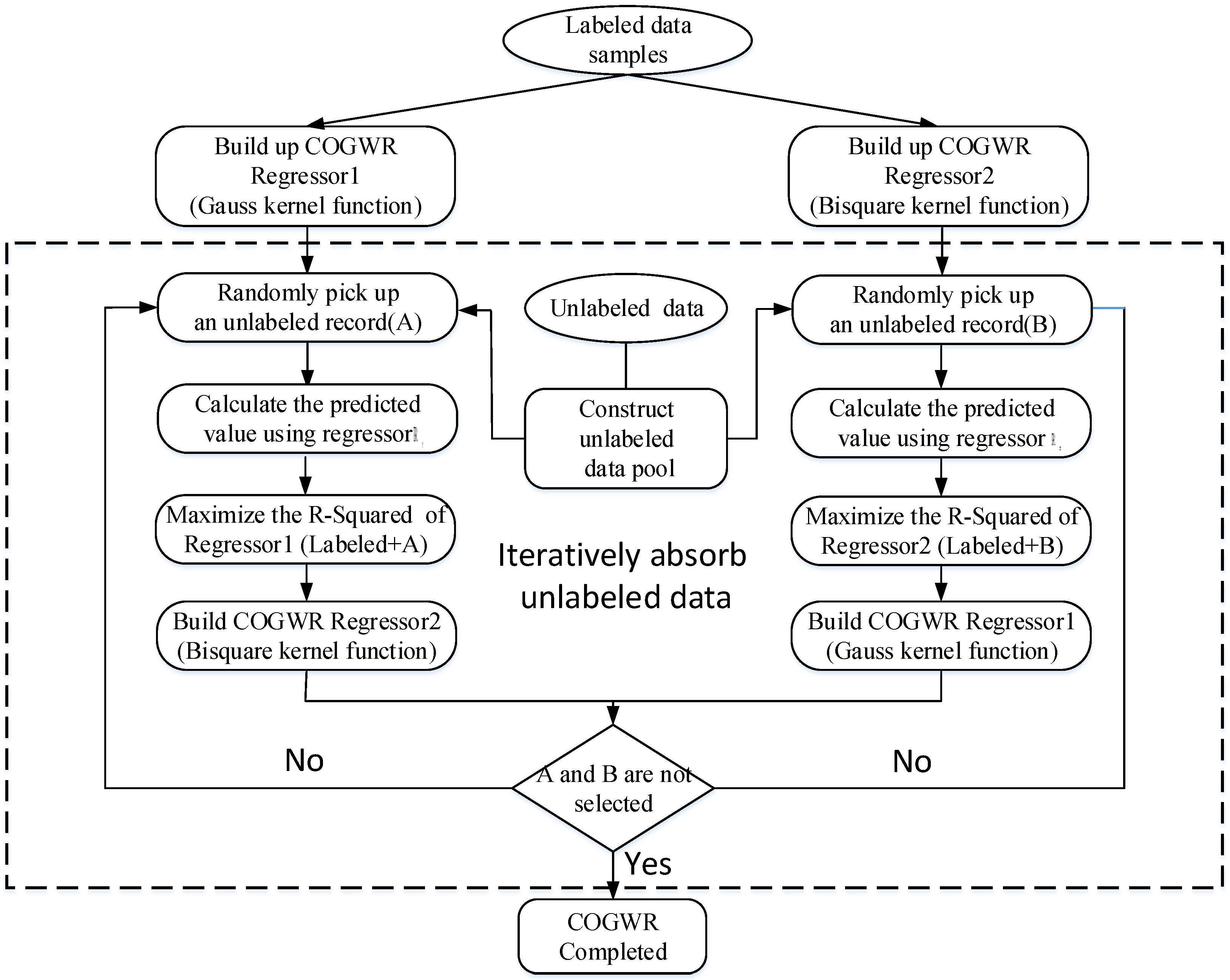
3.2.3. Co-Training Geographically-Weighted Regression Approach

Let $L=\left\{\left(x_1,y_1\right),\cdots ,\left(x_{\left|L\right|},y_{\left|L\right|}\right)\right\}$ denote the housing price sample set, where the i-th instance $x_i$ is described by d attributes, $y_i$ is the housing price value and $\left|L\right|$ is the number of real-value examples; let U denote the no real value dataset, where the instances are also described by d attributes, whose real values are unknown, and $\left|U\right|$ is the number of no real value examples. The procedure is described as follows:

1 Initialize: Build up the adaptive Gauss kernel co-training geographical weighted regression (COGWR) regressor $R_1$ and the adaptive bi-square kernel COGWR regressor $R_2$ with the labeled samples L. Randomly select a small number of unlabeled samples and construct an unlabeled data pool P.

2 Absorb unlabeled samples: In each round, select an unlabeled record r from the unlabeled data pool P.

(1)

Assign the predicted value $\widehat{y_r}$ of the no real value record using COGWR regressor $R_1$ and add the record to the COGWR regressor ${R_1}^{\prime }$. If the $R^2$ of ${R_1}^{\prime }$ decreases in relation to the original $R^2$ using Equation (2), this record will be absorbed by regressor ${R_2}^{\prime }$.

The goodness of r can be evaluated using the criterion shown in Equation (7).

$${\Delta }_r={\displaystyle \sum }_{X_i\in L}{\left(y_i-R_1\left(x_i\right)\right)}^2-{\displaystyle \sum }_{X_iϵL}{\left(y_i-{R_1}^{\prime }\left(x_i\right)\right)}^2$$

(7)

If the value of ${\Delta }_r$ is positive, then utilizing $\left(x_r,{\widehat{y}}_r\right)$ is beneficial.

(2)

Otherwise, assign the predicted value $\widehat{y_r}$ of the no real value record using the COGWR regressor $R_2$ and add the record to the COGWR regressor ${R_2}^{\prime }$. If the $R^2$ of ${R_2}^{\prime }$ decreases in relation to the original$R^2$, this record will be absorbed by the regressor.

The goodness of r can be evaluated using the criterion shown in Equation (8).

$${\Delta }_r={\displaystyle \sum }_{X_i\in L}{\left(y_i-R_2\left(x_i\right)\right)}^2-{\displaystyle \sum }_{X_iϵL}{\left(y_i-{R_2}^{\prime }\left(x_i\right)\right)}^2$$

(8)

If the value of ${\Delta }_r$ is positive, then utilizing $\left(x_r,{\widehat{y}}_r\right)$ is beneficial.

(3)

If the unlabeled record is absorbed by neither regressor $R_1$ nor regressor$R_2$, then end the iteration.

3 Predict: Calculate the average value of regressor $R_1$ and regressor $R_2$.

A flowchart of the COGWR approach is shown in Figure 3.

Figure 3. Flowchart of the co-training geographical weighted regression (COGWR) algorithm.

Figure 3. Flowchart of the co-training geographical weighted regression (COGWR) algorithm.

4. Experimental Results and Comparisons

In this section, the GWR model using Gaussian kernel functions to consider the spatial heterogeneity of housing price data was adopted to validate the reliability of housing price predictions in Beijing. Secondly, the housing price data were analyzed using the GWR and COGWR methods.

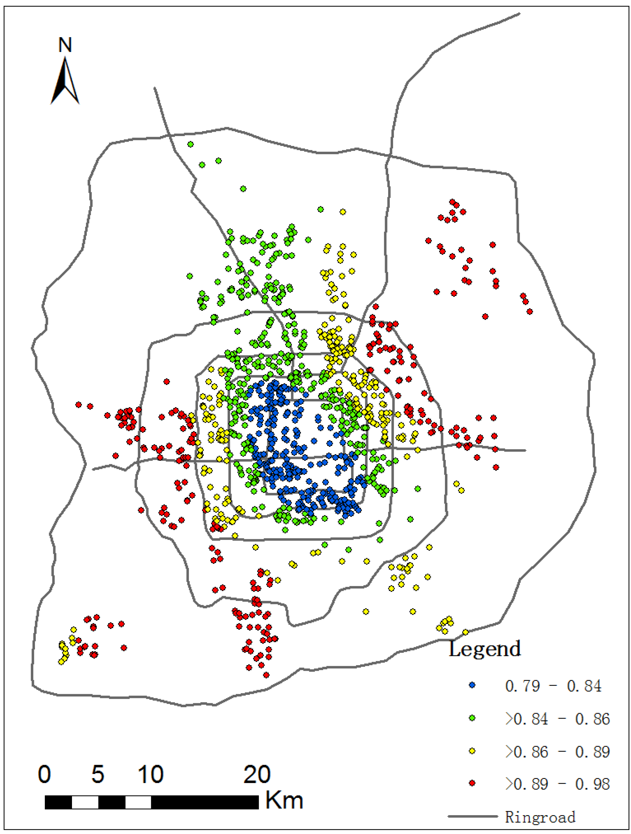
4.1. The Results of GWR Model

In linear regression models, strong collinearity between explanatory variables could increase the variance of the estimated regression coefficients and result in misleading conclusions about relationships in the phenomenon under study. In the local linear regression setting, this could lead to imprecise coefficient patterns with counter-intuitive signs in significant portions of the study area [39]. For example, Wheeler shows that collinearity can degrade coefficient precision in GWR and lead to counter-intuitive signs for some regression coefficients at some locations in the study area [40].

In this study, multicollinearity is diagnosed using the diagnostic tools of the variance inflation factor (VIF), condition index and variance-decomposition proportions. The VIF values are indicators for the severity of multicollinearity, and variables with VIF values greater than 10 should be eliminated. It is suggested by Belsley to use condition indexes greater than or equal to 30 and variance proportions greater than 0.50 for each variance component as an indication of collinearity in a regression model [41]. In this study, the VIF values of explanatory covariates are less than 10, and the condition index of all explanatory covariates and the intercept is less than 30.

It is known that an adaptive bandwidth has been proven to be highly suitable in practice compared to a predefined and fixed bandwidth [27,29]. In this experiment, the adaptive Gauss kernel function have been adopted. The GWR model is tested, and the results are shown in Table 2 [27,42,43]. The statistics indicate that housing prices in Beijing can be modeled using explanatory variables. Approximately 70.1% of the variation in housing prices could be explained by the model according to$R^2$. The signs for all of the parameters between the lower quartile (LQ) and upper quartile (UQ) are shown in Table 2. Descriptive statistics for the local parameter coefficients produced by GWR reveal much variance in the parameter values, suggesting the presence of spatial non-stationarity in the relationships between house prices and the explanatory variables. The floor area, number of baths and age of building at time of sale have positive parameter values, whereas the fee of property management, the plot ratio of houses, the green ratio and ringroad have both negative and positive parameter values.

Table 2. GWR model parameter estimate statistics. LQ, lower quartile; UQ, upper quartile.

Parameter	Min	LQ	Med	UQ	Max
constant	11.29	11.59	11.70	11.86	12.24
lnarea_total	0.79	0.84	0.86	0.89	0.98
nbath	0.02	0.08	0.10	0.13	0.17
lnpfee	−0.01	0.00	0.00	0.01	0.01
lnplotratio	−0.23	−0.19	−0.16	−0.13	−0.07
lngratio	−0.01	0.00	0.00	0.01	0.03
age	0.01	0.02	0.02	0.02	0.04
ringroad	−0.03	−0.01	0.00	0.01	0.02
Diagnostic information
R2		0.701
AdjustedR2		0.677
AIC		846.410

Table 2. GWR model parameter estimate statistics. LQ, lower quartile; UQ, upper quartile.

Parameter	Min	LQ	Med	UQ	Max
constant	11.29	11.59	11.70	11.86	12.24
lnarea_total	0.79	0.84	0.86	0.89	0.98
nbath	0.02	0.08	0.10	0.13	0.17
lnpfee	−0.01	0.00	0.00	0.01	0.01
lnplotratio	−0.23	−0.19	−0.16	−0.13	−0.07
lngratio	−0.01	0.00	0.00	0.01	0.03
age	0.01	0.02	0.02	0.02	0.04
ringroad	−0.03	−0.01	0.00	0.01	0.02
Diagnostic information
R2		0.701
AdjustedR2		0.677
AIC		846.410

For the test of non-stationarity, the F-test proposed by Leung et al. (2000) was conducted [42]. Table 3 lists the variances, F-statistic values of regression coefficients and their corresponding p-values. Those statistically-significant values at the 5% level are marked with an asterisk “*”. It can be found that only one variable exhibits nonsignificant spatial variations in GWR: the number of bath rooms (nbath). The remaining variables display significant spatial variations.

Table 3. The non-stationarity test results for the GWR models.

Parameter	Variance	F-statistic	p-Value
constant	7.221	37.620	<0.001 *
lnarea_total	0.029	2.417	<0.001 *
nbath	0.024	1.241	0.185
lnpfee	0.005	6.564	<0.001 *
lnplotratio	0.001	2.767	<0.001 *
lngratio	0.011	4.572	<0.001 *
age	0.000	3.956	<0.001 *
ringroad	0.624	149.913	<0.001 *

Note: * Denotes 5% statistical significance.

Table 3. The non-stationarity test results for the GWR models.

Parameter	Variance	F-statistic	p-Value
constant	7.221	37.620	<0.001 *
lnarea_total	0.029	2.417	<0.001 *
nbath	0.024	1.241	0.185
lnpfee	0.005	6.564	<0.001 *
lnplotratio	0.001	2.767	<0.001 *
lngratio	0.011	4.572	<0.001 *
age	0.000	3.956	<0.001 *
ringroad	0.624	149.913	<0.001 *

Note: * Denotes 5% statistical significance.

One important characteristic of the GWR-based technique is that the local parameter estimates that denote local relationships are mappable and thus allow for visual analysis. Taking the coefficients of logarithmically-transformed floor area as an example, we can group them into several intervals and color each interval to visualize the spatial variation patterns of this variable. As is shown in Figure 4, it could been seen that house prices are influenced by the floor area. In the central part of Beijing, a large amount of houses has been built with a small dwelling size. The reason is that central area of Beijing was planned in earlier times and no more land could be used to build houses. In recent years, with the fast development of the economy and the rapid progress of urbanization, a large-scale movement of urban expansion has emerged all over the country, and large-sized houses are built in the external part of Beijing.

Figure 4. Spatial variation of the logarithmically = transformed floor area coefficient.

Figure 4. Spatial variation of the logarithmically = transformed floor area coefficient.

4.2. Comparison of the COGWR with the GWR Model

In this paper, we have introduced an efficient semi-supervised regression approach to predict housing prices. A popular routine in evaluating semi-supervised algorithms is adopted [18,19]. In detail, the residential plots are randomly partitioned into labeled/unlabeled/test datasets according to certain ratios. About 25% of the data is kept as test examples, while the remaining 75% of the data is used as the set of training data. In the training set, labeled and unlabeled data are partitioned under different label rates including 10%, 20%, 30%, 40% and 50%. Fifty runs of the experiments are conducted; in each run, the RSS (Residual Sum of Squares), MSE (Mean Squared Error) and AIC values are recorded. In the experiments, the maximum number of iterations is set to 50, and the size of the pool used in the learning process is fixed to 50. Since the learning process may stop before the maximum number of iterations is reached, and in that case, the final RSS, MSE and AIC values are used in computing the average RSS, MSE and AIC values of the iterations.

It is necessary to investigate whether the COGWR model performs significantly better than the GWR models. The improvements of the RSS, MSE and AIC values between COGWR and GWR are shown in Table 4.

Table 4. Improvement between the COGWR and GWR models.

Comparison between Different Models		The Labeling Ratio of Housing Price Data
		10%	20%	30%	40%	50%
COGWR (Gauss kernel function) regressor/GWR Improvement	RSS	3.242	3.375	3.551	−0.144	−0.314
	MSE	0.010	0.010	0.011	0.000	−0.001
	AIC	23.716	36.479	41.921	−2.892	−4.812
COGWR (bi-square kernel function) regressor/GWR Improvement	RSS	2.216	2.801	2.909	0.101	−1.633
	MSE	0.007	0.008	0.009	0.000	−0.005
	AIC	18.645	21.328	22.899	2.204	−16.641

Table 4. Improvement between the COGWR and GWR models.

Comparison between Different Models		The Labeling Ratio of Housing Price Data
		10%	20%	30%	40%	50%
COGWR (Gauss kernel function) regressor/GWR Improvement	RSS	3.242	3.375	3.551	−0.144	−0.314
	MSE	0.010	0.010	0.011	0.000	−0.001
	AIC	23.716	36.479	41.921	−2.892	−4.812
COGWR (bi-square kernel function) regressor/GWR Improvement	RSS	2.216	2.801	2.909	0.101	−1.633
	MSE	0.007	0.008	0.009	0.000	−0.005
	AIC	18.645	21.328	22.899	2.204	−16.641

First, we compared RSS and MSE between COGWR and GWR. All COGWR regressors (Gauss and bi-square kernel functions) achieve better performance than the GWR regressors at the label rates of 10%, 20% and 30%. For instance, compared to the GWR regressors, the improvement in RSS achieved by the COGWR regressors was (3.242, 2.216), (3.375, 2.801) and (3.551, 2.909), respectively. However, for label rates of 40% and 50%, no significant improvement was observed when compared to the GWR regressor. For example, the improvement of RSS calculated using the COGWR regressor was (−0.144, 0.101) and (−0.314, −1.633), respectively.

Second, we compared AIC values between the COGWR and GWR models and determined whether the COGWR model is significantly more reliable than the GWR models. According to Fotheringham and Bo Wu [5,44], a “serious” difference between the two models is generally regarded as one in which the difference in AIC values between the models is greater than three. When the labeled rate is 10%, 20% or 30%, significant improvements are achieved by using the COGWR when compared to the GWR. For instance, when the label rate is 10%, 20% and 30%, the difference between the COGWR and GWR models was (23.716, 18.645), (36.479, 21.328) and (41.921, 22.899), respectively. However, no significant improvement is achieved by using the COGWR when the labeled rate is 40% or 50%. When the labeled rate is 40% and 50%, the difference between the COGWR and GWR is (−2.892, 2.204) and (−4.812, −16.641), respectively.

With the increasing of the label rate, the improvement of goodness-of-fit endowed by exploiting unlabeled house price data seems to be decreasing. This is not strange, since it can be perceived from the performance of labeling that the initial GWR regressors become robust when more labeled house price data are available and, therefore, are more difficult to enhance.

5. Conclusions

Traditional semi-supervised regression methods could not be directly applied to spatial data, since the assumption of stability over space is generally unrealistic. This paper introduced novel co-training GWR approaches, which fully utilize the advantages of both the geographical regression and the semi-supervised learners to increase the goodness-of-fit with respect to unlabeled house structural, locational and neighborhood characteristics and geographical data.

The COGWR model, which fully utilizes the positive aspects of both the geographical weighted regression (GWR) method and semi-supervised learning paradigm, was implemented, and the results reveal that when the amount of labeled data is small, the COGWR method significantly improves the performance of the GWR method. By absorbing unlabeled data, this method converts sparse data areas into dense data areas. Therefore, the robustness of the regressors is enhanced. This suggests that incorporating no-price data into a GWR model could yield meaningful results. When the label rate of housing price data increases, the gains from absorbing unlabeled data decrease because the regressors trained on the labeled training examples become stronger and are thus more difficult to improve.

This study is a beneficial attempt in the research of geo-information and real estate economics. It offers a reference to both the decision-making and the theoretical research. The spatial diversity of the regression coefficients is of utmost importance for locally-acting decision-makers [12]. When the amount of house price data is limited, the COGWR approach is a useful tool for real estate practitioners to fully exploit no-price data with explanatory variables.

Some limitations still remain in our study, and further work is required. In this paper, not all explanatory variables vary over space, and the mixed geographically-weighted regression (MGWR) approach should be investigated to prevent the limitations of fixed effects by exploring spatially-stationary and non-stationary effects in the future [12]. Spatiotemporal heterogeneity prevails in real estate data, and a temporal semi-supervised GWR must still be pursued.

References

1. Kim, K.; Park, J. Segmentation of the housing market and its determinants: Seoul and its neighbouring new towns in Korea. J. Aust. Geogr. 2005, 36, 221–232. [Google Scholar] [CrossRef]
2. Selim, S. Determinants of house prices in Turkey: A hedonic regression model. J. Doğuş Üniv. Dergisi. 2011, 9, 65–76. [Google Scholar]
3. Harris, R.; Dong, G.; Zhang, W. Using contextualized geographically weighted regression to model the spatial heterogeneity of land prices in Beijing, China. Trans. GIS 2013, 17, 901–919. [Google Scholar] [CrossRef]
4. Lu, B.; Charlton, M.; Harris, P.; Fotheringham, A.S. Geographically weighted regression with a non-euclidean distance metric: A case study using hedonic house price data. Int. J. Geogr. Inf. Sci. 2014, 28, 660–681. [Google Scholar] [CrossRef]
5. Wu, B.; Li, R.; Huang, B. A geographically and temporally weighted autoregressive model with application to housing prices. Int. J. Geogr. Inf. Sci. 2014, 28, 1186–1204. [Google Scholar] [CrossRef]
6. Brunsdon, C.; Fotheringham, A.S.; Charlton, M. Some notes on parametric significance tests for geographically weighted regression. J. Reg. Sci. 1999, 39, 497–524. [Google Scholar] [CrossRef]
7. Brunsdon, C.; Fotheringham, A.S.; Charlton, M.E. Geographically weighted regression: A method for exploring spatial nonstationarity. Geogr. Anal. 1996, 28, 281–298. [Google Scholar] [CrossRef]
8. Huang, Y.; Leung, Y. Analysing regional industrialisation in Jiangsu province using geographically weighted regression. J. Geogr. Syst. 2002, 4, 233–249. [Google Scholar] [CrossRef]
9. Bourassa, S.; Cantoni, E.; Hoesli, M. Predicting house prices with spatial dependence: A comparison of alternative methods. J. Real. Estate Ers 2010, 32, 139–159. [Google Scholar]
10. Dubin, R.A. Spatial autocorrelation: A primer. J. Hous. Econ. 1998, 7, 304–327. [Google Scholar] [CrossRef]
11. Redfearn, C.L. How informative are average effects? Hedonic regression and amenity capitalization in complex urban housing markets. Reg. Sci. Urban Econ. 2009, 39, 297–306. [Google Scholar]
12. Helbich, M.; Brunauer, W.; Caz, E.; Nijkamp, P. Spatial heterogeneity in hedonic house price models—The case of Austria. Urban Stud. 2014, 51, 390–411. [Google Scholar] [CrossRef]
13. LeSage, J.P. An introduction to spatial econometrics. Rev. Econ. Ind. 2008, 123, 19–44. [Google Scholar] [CrossRef]
14. Pace, R.K.; Gilley, O.W. Generalizing the OLS and grid estimators. R. Estate Econ. 1998, 26, 331–347. [Google Scholar] [CrossRef]
15. Goodman, A.C.; Thibodeau, T.G. Housing market segmentation and hedonic prediction accuracy. J. Hous. Econ. 2003, 12, 181–201. [Google Scholar] [CrossRef]
16. Blum, A.; Mitchell, T. Combining labeled and unlabeled data with co-training. In Proceedings of the 11th Annual Conference on Computational Learning Theory (ACM), Madison, WI, USA, 24–26 July 1998.
17. Brefeld, U.; Gärtner, T.; Scheffer, T.; Wrobel, S. (Eds.) Efficient co-regularised least squares regression. In Proceedings of the 23rd International Conference on Machine Learning (ACM), Pittsburgh, PA, USA, 25–29 June 2006.
18. Zhou, Z.H.; Li, M. Semi-supervised regression with co-training. In Proceedings of 2005 International Joint Conferences on Artificial Intelligence, Edinburgh, Scotland, 30 July–5 August 2005.
19. Zhou, Z.H.; Li, M. Semisupervised regression with cotraining-style algorithms. IEEE Trans. Knowl. Data Eng. 2007, 19, 1479–1493. [Google Scholar] [CrossRef]
20. Tan, K.; Li, E.; Du, Q.; Du, P. An efficient semi-supervised classification approach for hyperspectral imagery. ISPRS J. Photogram. Remote Sens. 2014, 97, 36–45. [Google Scholar] [CrossRef]
21. Huang, B.; Wu, B.; Barry, M. Geographically and temporally weighted regression for modeling spatio-temporal variation in house prices. Int. J. Geogr. Inf. Sci. 2010, 24, 383–401. [Google Scholar] [CrossRef]
22. Goodman, A.C. Andrew Court and the invention of hedonic price analysis. J. Urban Econ. 1998, 44, 291–298. [Google Scholar] [CrossRef]
23. Yu, D.; Wei, Y.D.; Wu, C. Modeling spatial dimensions of housing prices in Milwaukee, WI. Environ. Plan. B 2007, 34, 1085–1102. [Google Scholar] [CrossRef]
24. Ustaoğlu, E. Hedonic Price Analysis of Office Rents: A Case Study of the Office Market in Ankara. Master Thesis, Middle East Technical University, Ankara, Turkey, 2003. [Google Scholar]
25. Rosen, S. Hedonic prices and implicit markets: Product differentiation in pure competition. J. Polit. Econ. 1974, 82, 34–55. [Google Scholar] [CrossRef]
26. Farber, S.; Yeates, M. A comparison of localized regression models in a hedonic house price context. Can. J. Reg. Sci. 2006, 29, 405–420. [Google Scholar]
27. McMillen, D.P.; Redfearn, C.L. Estimation and hypothesis testing for nonparametric hedonic house price functions. J. Reg. Sci. 2010, 50, 712–733. [Google Scholar] [CrossRef]
28. Helbich, M.; Brunauer, W.; Hagenauer, J.; Leitner, M. Data-driven regionalization of housing markets. Ann. Assoc. Am. Geogr. 2013, 103, 871–889. [Google Scholar] [CrossRef]
29. Guan, J.; Zurada, J. An adaptive neuro-fuzzy inference system based approach to real estate property assessment. J. Real Estate Res. 2008, 30, 395–421. [Google Scholar]
30. Peterson, S.; Flanagan, A. Neural network hedonic pricing models in mass real estate appraisal. J. Real Estate Res. 2009, 31, 147–164. [Google Scholar]
31. Kuşan, H.; Aytekin, O.; Özdemir, İ. The use of fuzzy logic in predicting house selling price. Expert Syst. Appl. 2010, 37, 1808–1813. [Google Scholar] [CrossRef]
32. Kestens, Y.; Thériault, M.; Des Rosiers, F. Heterogeneity in hedonic modelling of house prices: Looking at buyers’ household profiles. J. Geogr. Syst. 2006, 8, 61–96. [Google Scholar] [CrossRef]
33. Zheng, S.; Kahn, M.E. Land and residential property markets in a booming economy: New evidence from Beijing. J. Urban Econ. 2008, 63, 743–757. [Google Scholar] [CrossRef]
34. Zhou, Z.; Li, M. Semi-supervised learning by disagreement. Knowl. Inf. Syst. 2010, 24, 415–439. [Google Scholar] [CrossRef]
35. Páez, A.; Long, F.; Farber, S. Moving window approaches for hedonic price estimation: An empirical comparison of modelling techniques. Urban Stud. 2008, 45, 1565–1581. [Google Scholar] [CrossRef]
36. Goldman, S.; Zhou, Y. Enhancing supervised learning with unlabeled data. In Proceedings of the Seventeenth International Conference on Machine Learning, Stanford, CA, USA, 21–23 June 1990.
37. Zhou, Z.; Li, M. Tri-training: Exploiting unlabeled data using three classifiers. IEEE Trans. Knowl. Data Eng. 2005, 17, 1529–1541. [Google Scholar] [CrossRef]
38. Li, M.; Zhou, Z. Improve computer-aided diagnosis with machine learning techniques using undiagnosed samples. IEEE Trans. Syst. Man Cybern. A 2007, 37, 1088–1098. [Google Scholar] [CrossRef]
39. Wheeler, D.C. Diagnostic tools and a remedial method for collinearity in geographically weighted regression. Environ. Plan. A 2007, 39, 2464. [Google Scholar] [CrossRef]
40. Wheeler, D.; Tiefelsdorf, M. Multicollinearity and correlation among local regression coefficients in geographically weighted regression. J. Geogr. Syst. 2005, 7, 161–187. [Google Scholar] [CrossRef]
41. David, B. Conditioning Diagnostics, Collinearity and Weak Data in Regression; John Wiley & Sons: Hobokon, NJ, USA, 1991. [Google Scholar]
42. Leung, Y.; Mei, C.; Zhang, W. Statistical tests for spatial nonstationarity based on the geographically weighted regression model. Environ. Plan. A 2000, 32, 9–32. [Google Scholar] [CrossRef]
43. Zhao, N.; Yang, Y.; Zhou, X. Application of geographically weighted regression in estimating the effect of climate and site conditions on vegetation distribution in Haihe catchment, China. Plant Ecol. 2010, 209, 349–359. [Google Scholar] [CrossRef]
44. Fotheringham, A.S.; Brunsdon, C.; Charlton, M. Geographically Weighted Regression: The Analysis of Spatially Varying Relationship; Wiley: Chichester, UK, 2003. [Google Scholar]