
A Two-Step Clustering Approach to Extract Locations from Individual GPS Trajectory Data


Abstract
:1. Introduction
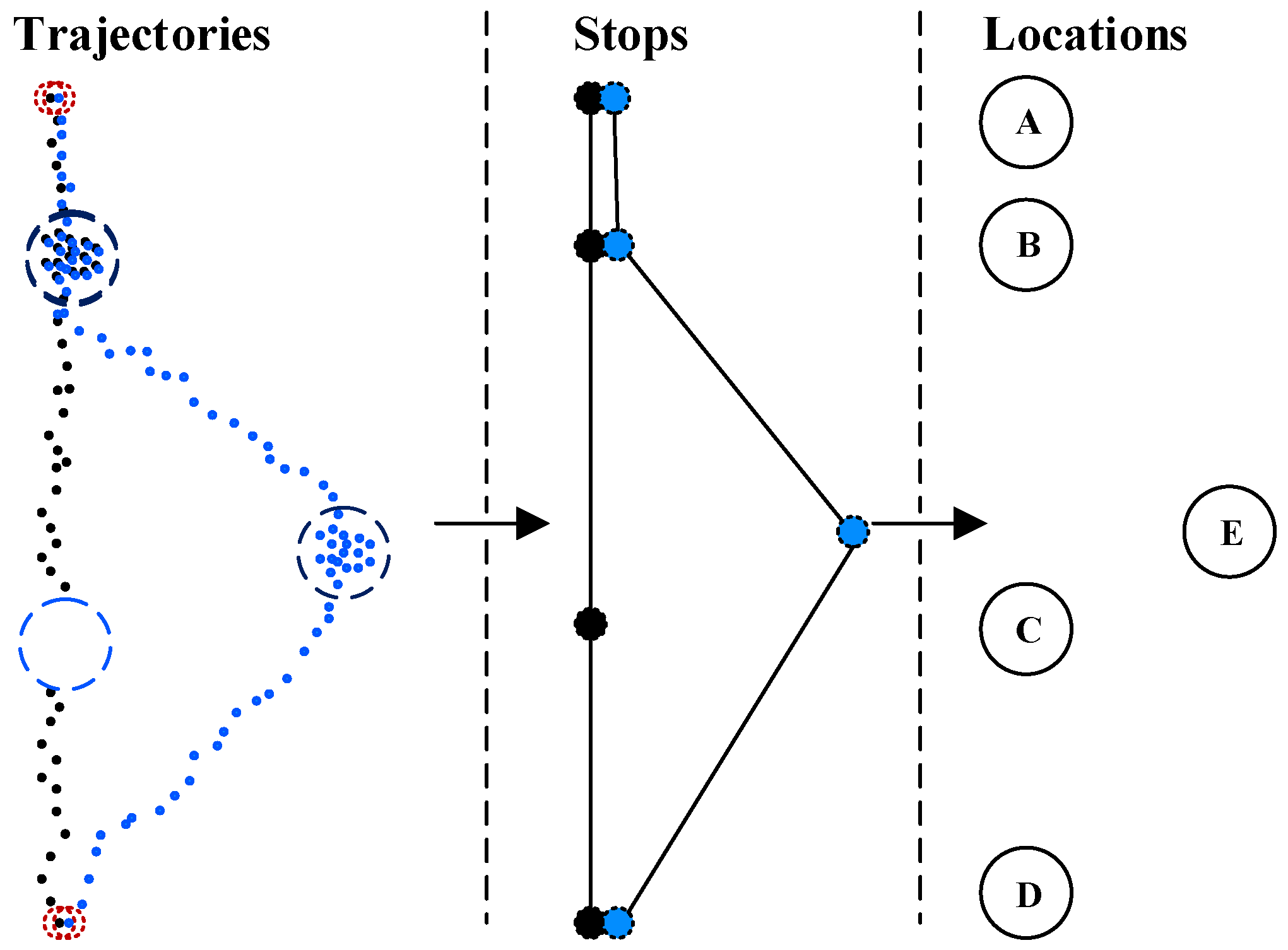
2. Location Extraction
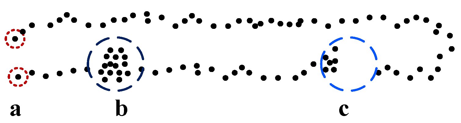
2.1. Extracting Stop Points
| Algorithm 1. Stop Point Extraction (TDBC) | ||
| Input: Trajectory T, time threshold δt, distance threshold δd | ||
| Output: a set of stop points SP | ||
| 1: | Cluster=; Previous C=; | |
| 2: | if the first or last point is type I then SP.add(the point); | // type I |
| 3: | for each point Pi in T do | |
| 4: | if distance(Cluster, Pi) < δd then put Pi in Cluster; continue; | |
| 5: | if distance(Cluster, Pi) > δd and duration(Cluster) > δt then | |
| 6: | SP.add(Cluster); continue; | // type II |
| 7: | if distance(Cluster, Pi) > δd and duration(Cluster) < δt then | |
| 8: | check(Cluster, Previous C); continue; | |
| 9: | if distance(Pi-1, Pi) < δd and duration(Pi-1, Pi) > δt then | |
| 10: | SP.add({Pi-1, Pi}); continue; | // type III |
| 11: | if distance(Pi-1, Pi) > δd and duration(Pi-1, Pi) > δt then ignore(); | |
| 12: | return SP; | |
| Function check(Cluster, Previous Cluster){ | ||
| if (time interval(Cluster, Previous) < δt and distance(Cluster, Previous) < δd) then | ||
| Previous = merge(Cluster, Previous); | ||
| if Previous is one of type II then SP.add(Previous); | ||
| else Previous = Cluster;} | ||
| Function SP.add(Cluster){ | ||
| if (distance(Cluster, Previous stop point in SP) < δd) then | ||
| Previous = merge(Cluster, Previous); | ||
| else put Cluster in SP; Previous = Cluster;} | ||
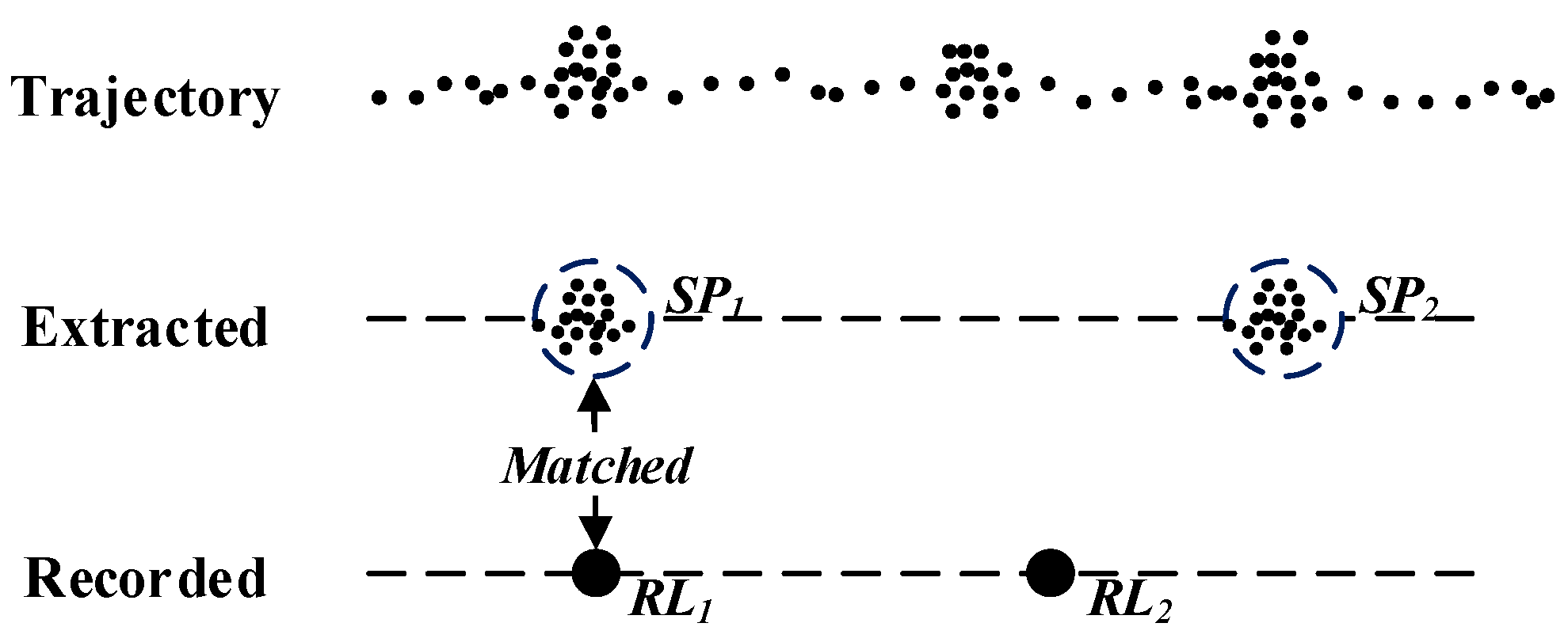
2.2. Extracting Locations
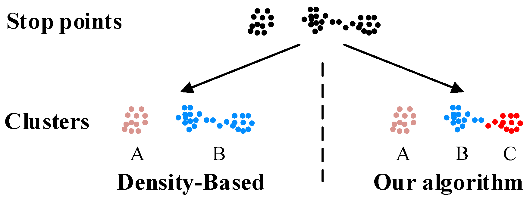
2.2.1. Clustering by Fast Search and Find of Density Peak
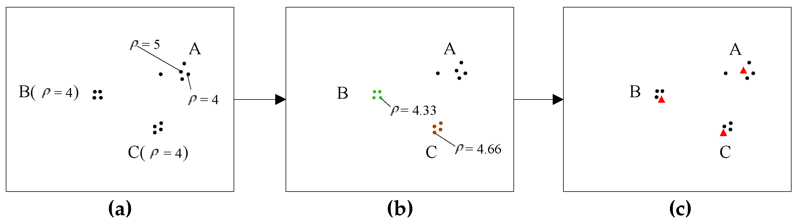
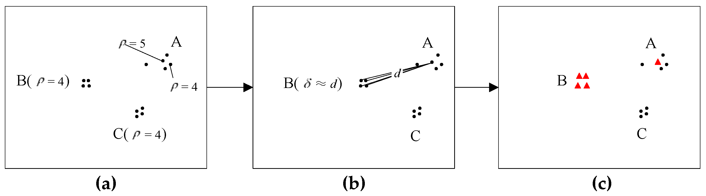
2.2.2. Problem Interpretation and Algorithm Improvement
- (1)
- a = max().
- (2)
- Take out the points with the same density a, and process each point by the following steps 3 and 4.
- (3)
- For point SPi with the density a, check the density of each point in neighbor Ni. If there is a point in Ni which the density is higher than a, ignore the point SPi, otherwise put it into the set S( = a).
- (4)
- For each point with the density a in neighbor Ni, repeat Steps 3 and 4 until all the points with the density a have been processed and form the set S( = a) = {SPi, …, SPj, …, SPk}.
- (5)
- For each point in the set S, check the neighbor relationship with each other. If two points are neighborhood, put them into a subset SBj. Then, form the set S = {SB1, …, SBm}, SBj = {SPl, …, SPk}, which contains m subsets. For each subset, the points are adjacent to each other and have the same density a.
- (6)
- For each subset SBi, pick a point randomly and make its density equal to ρi = a + i/(m+1).
- (7)
- a = a − 1, repeat Steps 2 to 7. If a = 1, the algorithm is terminated.
3. Experimental Section
3.1. Data Acquisition
3.2. Preprocessing
| Algorithm 2. Pre-processing | |
| Input: Trajectory T, speed threshold δv, altitude threshold δalt, satellites threshold δsatellites, HDOP threshold δhdop | |
| Output: T without outliers | |
| 1: | previous point = P0; |
| 2: | for each point Pi in T do |
| 3: | vi = distance(previous point, Pi) / duration(previous point, Pi); |
| 4: | if vi > δv or Pi.alt > δalt or Pi.satellites < δsatellites or Pi.HDOP > δhdop then |
| 5: | remove Pi from T; |
| 6: | else previous point = Pi; |
| 7: | return T; |
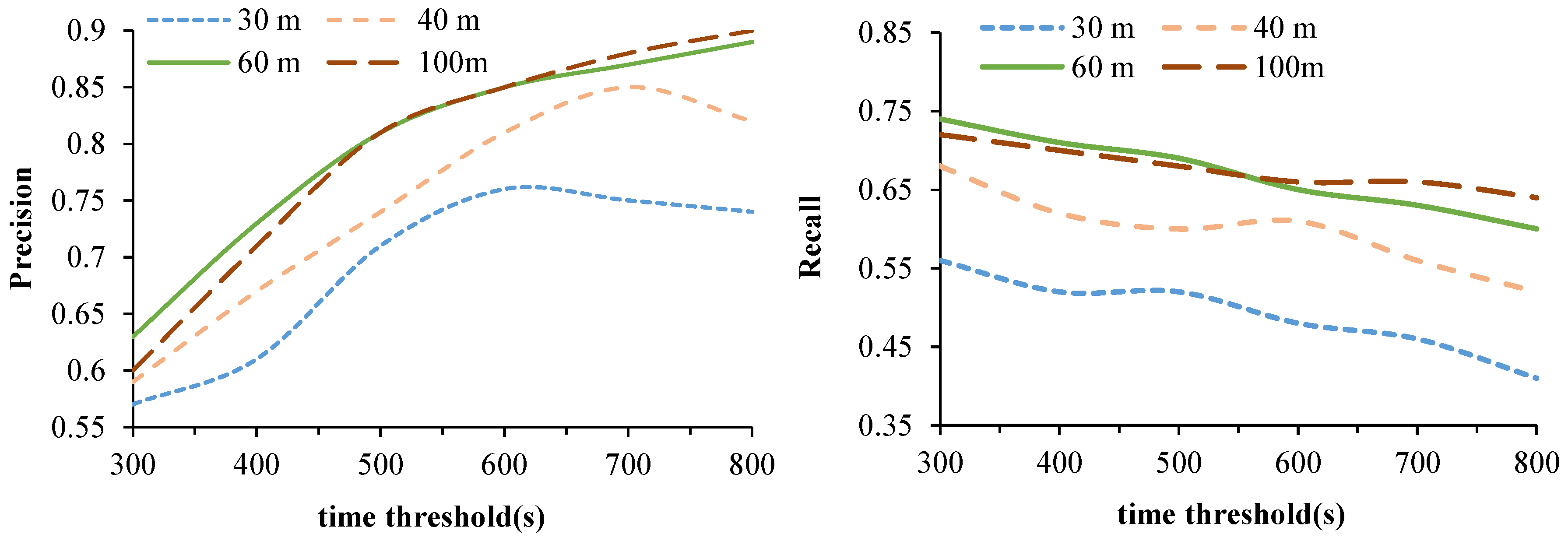
3.3. Parameters
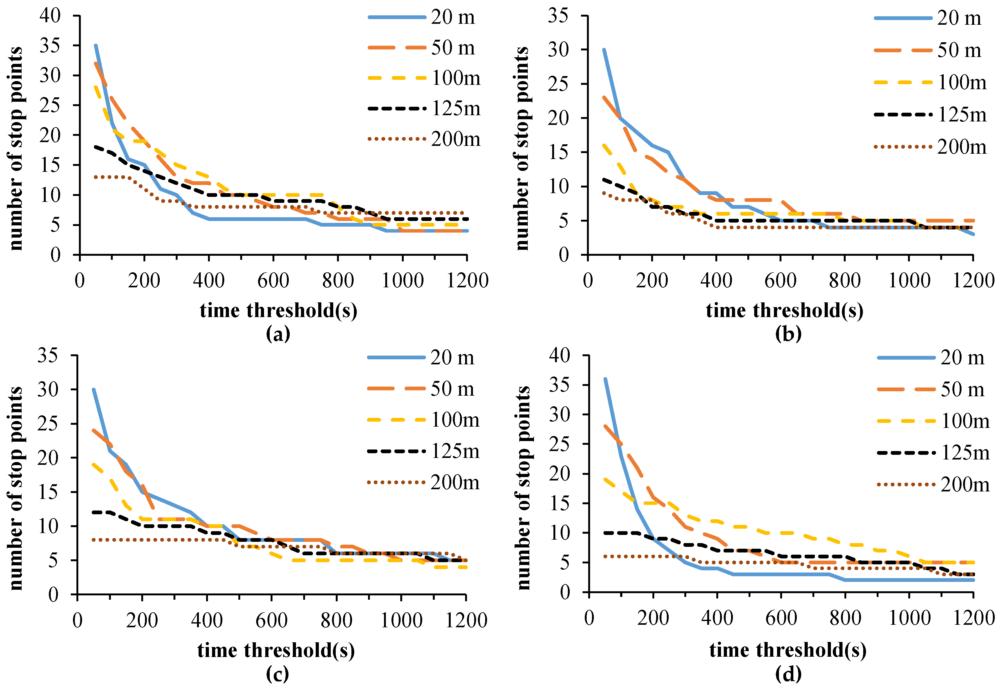
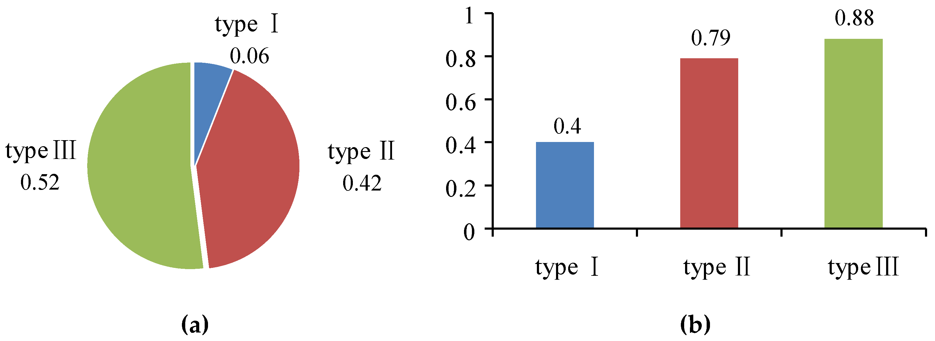
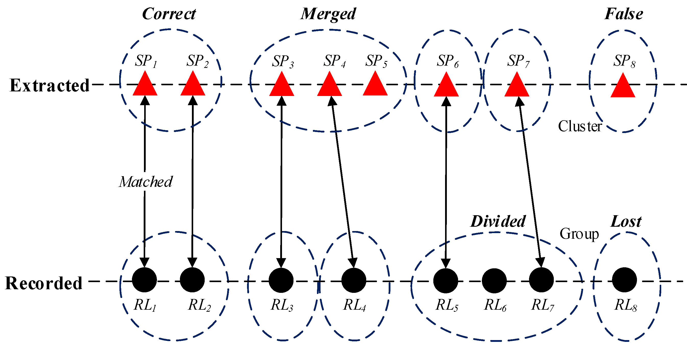
3.4. Stop Point Extraction Experiment
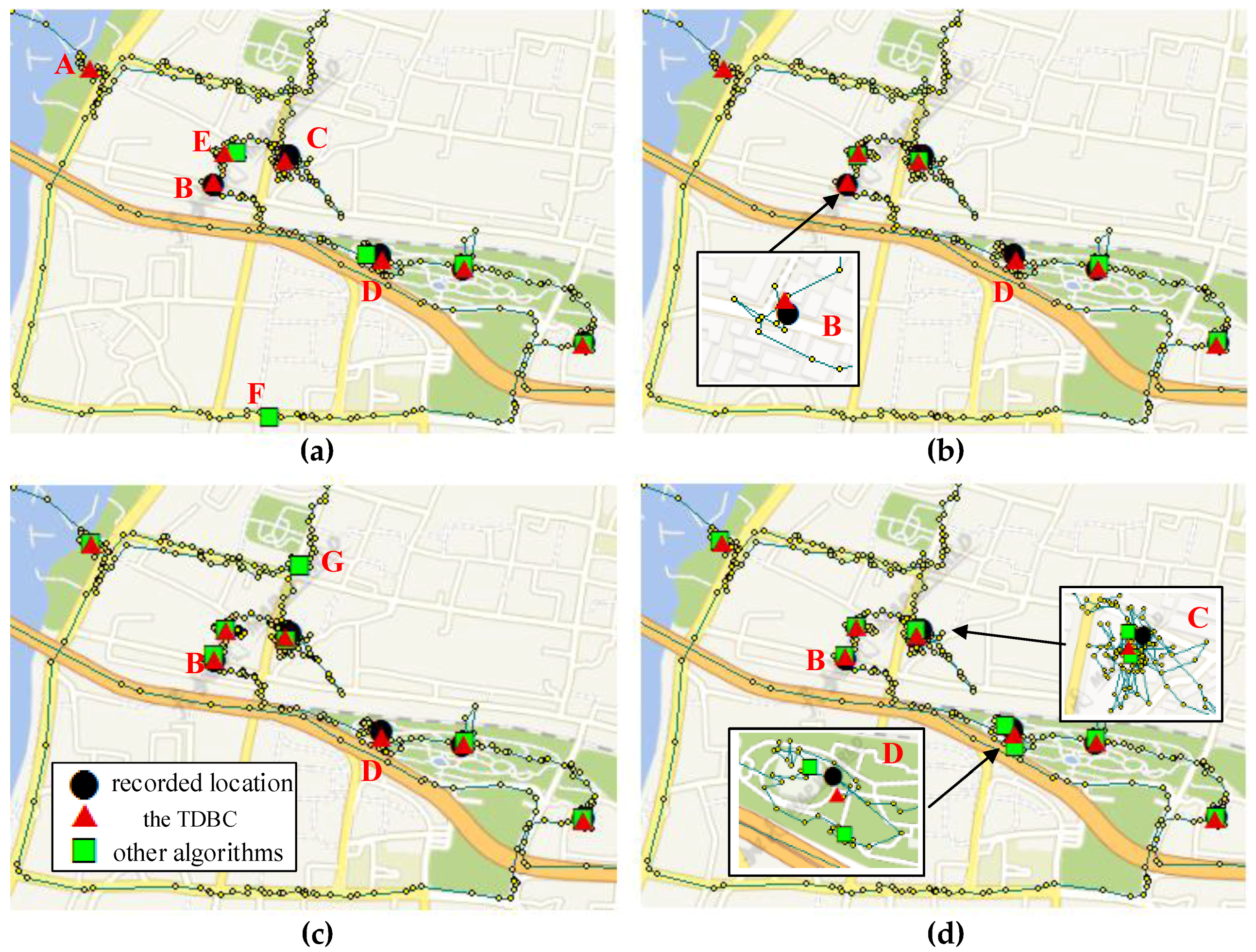
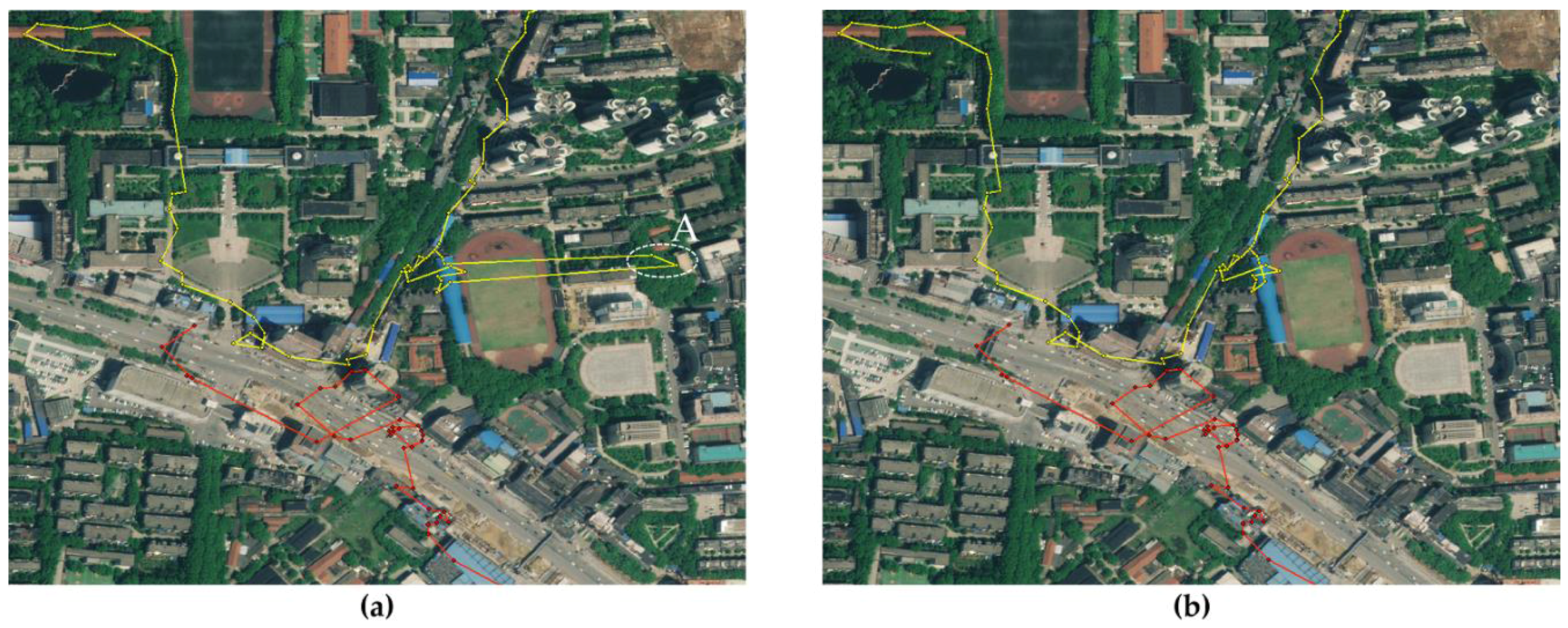
3.5. Location Extracting Experiment
4. Conclusions and Future Work
Acknowledgments
Author Contributions
Conflicts of Interest
References
- González, M.C.; Hidalgo, C.A.; Barabási, A.L. Understanding individual human mobility patterns. Nature 2008, 453, 779–782. [Google Scholar] [CrossRef] [PubMed]
- Harrison, S.; Dourish, P. Re-place-ing space: The roles of place and space in collaborative systems. In Proceedings of the 1996 ACM Conference on Computer Supported Cooperative Work, Boston, MA, USA, 16–20 November 1996.
- Lv, M.; Chen, L.; Xu, Z.; Li, Y.; Chen, G. The discovery of personally semantic places based on trajectory data mining. Neurocomputing 2016, 173, 1142–1153. [Google Scholar] [CrossRef]
- Yu, Y.; Kim, J.; Shin, K.; Jo, G.S. Recommendation system using location-based ontology on wireless internet: An example of collective intelligence by using ‘mashup’applications. Expert Syst. Appl. 2009, 36, 11675–11681. [Google Scholar] [CrossRef]
- Stopher, P.R.; Jiang, Q.; FitzGerald, C. Processing GPS data from travel surveys. In Proceedings of the Second International Colloqium on the Behavioural Foundations of Integrated Land-Use and Transportation Models: Frameworks, Models and Applications, Toronto, ON, Canada, 12–15 June 2005.
- Chen, L.; Lv, M.; Chen, G. A system for destination and future route prediction based on trajectory mining. Pervasive Mob. Comput. 2010, 6, 657–676. [Google Scholar] [CrossRef]
- Zhang, J.; Zhu, M.; Papadias, D.; Tao, Y.; Lee, D.L. Location-based spatial queries. In Proceedings of the 2003 ACM SIGMOD International Conference on Management of Data, San Diego, CA, USA, 10–12 June 2003.
- Kim, D.H.; Hightower, J.; Govindan, R.; Estrin, D. Discovering semantically meaningful places from pervasive rf-beacons. In Proceedings of the 11th international conference on Ubiquitous Computing, Orlando, FL, USA, 30 September–3 October 2009.
- Hightower, J.; Consolvo, S.; LaMarca, A.; Smith, I.; Hughes, J. Learning and recognizing the places we go. In Proceedings of the Ubicomp 2005: Ubiquitous Computing, Tokyo, Japan, 11–14 September 2005.
- Paek, J.; Kim, J.; Govindan, R. Energy-efficient rate-adaptive GPS-based positioning for smartphones. In Proceedings of the 8th International Conference on Mobile Systems, Applications, and Services, San Francisco, CA, USA, 15–18 June 2010.
- Schuessler, N.; Axhausen, K. Processing raw data from global positioning systems without additional information. Transp. Res. Rec. J. Transp. Res. Board 2009. [Google Scholar] [CrossRef]
- Ashbrook, D.; Starner, T. Learning significant locations and predicting user movement with GPS. In Proceedings of the Sixth International Symposium, Vienna, Austria, 21–23 April 2002.
- Zhou, C.; Frankowski, D.; Ludford, P.; Shekhar, S.; Terveen, L. Discovering personally meaningful places: An interactive clustering approach. ACM Trans. Inf. Syst. (TOIS) 2007. [Google Scholar] [CrossRef]
- Ester, M.; Kriegel, H.-P.; Sander, J.; Xu, X. A density-based algorithm for discovering clusters in large spatial databases with noise. In Proceedings of the 2nd International Conference on Knowledge Discovery and Data Mining, Portland, OR, USA, 2–4 August 1996.
- Ashbrook, D.; Starner, T. Using GPS to learn significant locations and predict movement across multiple users. Pers. Ubiquitous Comput. 2003, 7, 275–286. [Google Scholar] [CrossRef]
- Du, J.; Aultman-Hall, L. Increasing the accuracy of trip rate information from passive multi-day GPS travel datasets: Automatic trip end identification issues. Transp. Res. Part A Policy Pract. 2007, 41, 220–232. [Google Scholar] [CrossRef]
- Kang, J.H.; Welbourne, W.; Stewart, B.; Borriello, G. Extracting places from traces of locations. In Proceedings of the 2nd ACM International Workshop on Wireless Mobile Applications and Services on WLAN Hotspots, Philadelphia, PA, USA, 1 October 2004.
- Alvares, L.O.; Bogorny, V.; Kuijpers, B.; de Macedo, J.A.F.; Moelans, B.; Vaisman, A. A model for enriching trajectories with semantic geographical information. In Proceedings of the 15th annual ACM International Symposium on Advances in Geographic Information Systems, Seattle, WA, USA, 7–9 November 2007.
- Palma, A.T.; Bogorny, V.; Kuijpers, B.; Alvares, L.O. A clustering-based approach for discovering interesting places in trajectories. In Proceedings of the 2008 ACM Symposium on Applied Computing, Ceará, Brazil, 16–20 March 2008.
- Yuan, H.; Qian, Y.; Yang, R. Research on GPS-trajectory-based personalization poi and path mining. Syst. Eng. Theory Pract. 2015, 35, 1276–1282. [Google Scholar]
- Zaïane, O.R.; Foss, A.; Lee, C.H.; Wang, W. On data clustering analysis: Scalability, constraints, and validation. In Proceedings of the Pacific-Asia Conference on Knowledge Discovery and Data Mining, Taipei, Taiwan, 6–8 May 2002.
- Rodriguez, A.; Laio, A. Clustering by fast search and find of density peaks. Science 2014, 344, 1492–1496. [Google Scholar] [CrossRef] [PubMed]


| Raw Data | Filtered Data | Dataset 1 | Dataset 2 | Dataset 3 | |
|---|---|---|---|---|---|
| Volunteers | 23 | 23 | 11 | 4 | 1 |
| Days | 26 | 22 | 20 | 1 | 1 |
| GPS points | 441,715 | 383,660 | 205,612 | 3726 | 1043 |
| Recorded Locations | 2863 | 2657 | 1541 | 31 | 9 |
| TDBC | K-Medoids | DJ-Cluster | CB-SMoT | Time-Based | |
|---|---|---|---|---|---|
| Parameters | d = 60 m t = 500 s | K = 6 | eps = 60 m minPoint = 30 | area = 0.3 time = 300 s | d = 60 m t = 500 s |
| Time Complexity | O(n) | O(t(n-k)2) | O(tnlogn) | O(n2) | O(n) |
| Elapsed Time (s) | 0.9 | 198.52 | 194.47 | 81.9 | 0.97 |
| Precision | 0.81 | 0.45 | 0.84 | 0.58 | 0.54 |
| Recall | 0.68 | 0.60 | 0.58 | 0.66 | 0.61 |
| TDBC | K-Medoids | DJ-Cluster | CB-SMoT | Time-Based | |
|---|---|---|---|---|---|
| Parameters | d =60 m t = 500 s | K = 9 | eps = 60 m minPoint = 30 | area = 0.3 time = 300 s | d = 60 m t = 500 s |
| Recorded | 9 | 9 | 9 | 9 | 9 |
| Extracted | 10 | 9 | 6 | 11 | 12 |
| Matched | 7 | 4 | 5 | 6 | 6 |
| Precision | 0.7 | 0.44 | 0.83 | 0.55 | 0.5 |
| Recall | 0.78 | 0.44 | 0.56 | 0.66 | 0.66 |
| Our Algorithm | Density-Based | |
|---|---|---|
| Parameters | d = 60 m | eps = 60 m |
| Elapsed Time (s) | 0.351 | 1.912 |
| FR | 0.084 | 0.084 |
| MR | 0.056 | 0.167 |
| LR | 0.163 | 0.186 |
| DR | 0.116 | 0.07 |
| P | 0.722 | 0.694 |
| R | 0.605 | 0.618 |
| F | 0.658 | 0.654 |
© 2016 by the authors; licensee MDPI, Basel, Switzerland. This article is an open access article distributed under the terms and conditions of the Creative Commons Attribution (CC-BY) license (http://creativecommons.org/licenses/by/4.0/).
Share and Cite
Fu, Z.; Tian, Z.; Xu, Y.; Qiao, C. A Two-Step Clustering Approach to Extract Locations from Individual GPS Trajectory Data. ISPRS Int. J. Geo-Inf. 2016, 5, 166. https://0-doi-org.brum.beds.ac.uk/10.3390/ijgi5100166
Fu Z, Tian Z, Xu Y, Qiao C. A Two-Step Clustering Approach to Extract Locations from Individual GPS Trajectory Data. ISPRS International Journal of Geo-Information. 2016; 5(10):166. https://0-doi-org.brum.beds.ac.uk/10.3390/ijgi5100166
Chicago/Turabian StyleFu, Zhongliang, Zongshun Tian, Yanqing Xu, and Changjian Qiao. 2016. "A Two-Step Clustering Approach to Extract Locations from Individual GPS Trajectory Data" ISPRS International Journal of Geo-Information 5, no. 10: 166. https://0-doi-org.brum.beds.ac.uk/10.3390/ijgi5100166