Field Motion Estimation with a Geosensor Network ^†

Abstract

Physical environmental processes, such as the evolution of precipitation or the diffusion of chemical clouds in the atmosphere, can be approximated by numerical models based on the underlying physics, e.g., for the purpose of prediction. As the modeling process is often very complex and resource demanding, such models are sometimes replaced by those that use historic and current data for calibration. For atmospheric (e.g., precipitation) or oceanographic (e.g., sea surface temperature) fields, the data-driven methods often concern the horizontal displacement driven by transport processes (called advection). These methods rely on flow fields estimated from images of the phenomenon by computer vision techniques, such as optical flow (OF). In this work, an algorithm is proposed for estimating the motion of spatio-temporal fields with the nodes of a geosensor network (GSN) deployed in situ when images are not available. The approach adapts a well-known raster-based OF algorithm to the specifics of GSNs, especially to the spatial irregularity of data. In this paper, the previously introduced approach has been further developed by introducing an error model that derives probabilistic error measures based on spatial node configuration. Further, a more generic motion model is provided, as well as comprehensive simulations that illustrate the performance of the algorithm in different conditions (fields, motion behaviors, node densities and deployments) for the two error measures of motion direction and motion speed. Finally, the algorithm is applied to data sampled from weather radar images, and the algorithm performance is compared to that of a state-of-the-art OF algorithm applied to the weather radar images directly, as often done in nowcasting.

1. Introduction

The physical processes in the atmosphere or in the ocean, such as the evolution of precipitation, the water flow, the diffusion of chemical clouds in the atmosphere, etc., can be modeled by differential equations, for example, for the purpose of prediction. These models are usually called physical models. However, the modeling process is often very complex due to the influence of numerous factors that can often only be approximated, such as thermodynamic effects, solar radiation or the effects of terrain. Further, for computer processing, it is necessary to solve the usually complex differential equations numerically, for example, by using numerical weather prediction models, which requires the use of high-performance computational resources. Therefore, in certain applications, the physical models are replaced by data-driven methods that use historic or current data for calibration without the need to model the underlying physics [1]. An example of such data-driven or empirical models is the artificial neural network-based model for rainfall-runoff prediction in hydrology [2].

For atmospheric or oceanographic fields, the data-driven methods often concern the horizontal displacement of the features or fields (called advection). These methods often rely on motion fields estimated from the current and recent past data by computer vision techniques, such as optical flow (OF), and, when prediction is the goal, on the subsequent extrapolation in time using the motion information. Figure 1 displays a time series of weather radar images separated by 20 min (left to right) and motion vectors estimated using an image-based OF algorithm (the OpenCV implementation of the algorithm provided by [3]).

Sometimes, especially for short time scales, the data-driven, motion-based methods not only reduce computational demands, but also outperform the numerical models. In [4], it could be shown that the radar-based nowcasting of precipitation outperforms numerical prediction models for time scales below 6 h. There are numerous approaches that employ estimated motion vectors, not only for prediction as done in [5]. For example, in [6], it is shown that including motion information estimated from weather radar in the interpolation of rain gauge measurements improves the interpolation quality. Another example is the estimation of motion fields from remote sensing, e.g., from oceanographic satellite images. In [7], an approach to derive the surface ocean circulation from infra-red sea surface temperature measurements collected remotely by a satellite is introduced. The derived motion field is then further processed in order to derive representations of the fields without the need for physical models (an example mentioned is the derivation of the stationary points of the flow field, such as the center point of a hurricane). All of these approaches are similar in that motion vector fields are estimated from images of environmental phenomena. However, images are not always available, but only point measurements collected by in situ sensors. Examples include rain gauge measurements of precipitation, estimates of precipitation provided by cars ([8] or [9]) or sea surface temperature measurements collected by weather buoys.

In this work, it is investigated how the motion of spatio-temporal dynamic fields can be estimated by in situ sensors that are irregularly distributed in space. The sensors are assumed to be attached to computing and communication facilities and are therefore considered as the communicating nodes of a geosensor network (GSN). A well-known optical flow algorithm is used as a basis and adjusted to the specifics of GSNs and spatio-temporal fields, such as the irregularity of samples, the strong constraints on communication and computation and the assumed motion constancy over sampling periods. This way, the pixels in images translate to field samples collected by a node, and the pixel neighborhood translates to the node neighborhood in the GSN. The main differences of the approach compared to optical flow calculated from arbitrary images can be summarized as follows:

• A priori knowledge of motion properties: For the motion of environmental phenomena, a priori knowledge of the field motion properties can be assumed. For example, wind speed statistics exist or information on the advection of rainclouds. This domain knowledge can be used to specify the required parameters of the proposed algorithm.
• Temporal continuity and spatial uniformity of motion: In arbitrary images, moving objects, such as cars, can occur that change their direction, stop or accelerate rather quickly, e.g., within a couple of frames. Therefore, temporal continuity usually only holds for very short time periods [10]. For atmospheric or oceanographic fields, it is likely that the motion is rather consistent over long sampling periods, and therefore, integration of motion information over time gains importance. In addition, motion in images often exhibits sharp motion discontinuities, e.g., at boundaries of the moving objects such as cars with opposing motion that pass by each other. For atmospheric or oceanographic fields, sharp motion discontinuities can be considered unlikely: they might only arise at boundaries of the field, e.g., at the boundaries of rain clouds. However, then, they do not exist in reality (i.e., the atmosphere surrounding the rain cloud also moves), but affect the motion estimation algorithm that is based on field measurements. For example, while the atmosphere still moves when there is no rain, the motion can only be estimated when there is some rain, which is not uniform (the uniformity of the field values is commonly known as the “blank wall” problem in the optical flow literature).
• Controlled node deployment, sampling rate and irregular data: In image-based optical flow, the pixels determine the sampling locations, and the motion speed and direction are influenced by numerous factors, such as spatial resolution and the orientation of the image, sampling rate, the spatial distance of the camera to the moving object, as well as the speed and direction of the moving object. When motion is to be estimated with a GSN deployed within (i.e., in situ) and sensing the field, the node deployment and sampling rate can be controlled to a certain extent, for example, the node spacing relative to the assumed field motion. However, while image-based optical flow approaches usually rely on regular grids (i.e., images), a grid-like deployment of the nodes might not be possible.
• Decentralized estimation: Image-based OF usually relies on a single computer that estimates the motion field from the images. With a GSN, the decentralized estimation of motion by each node is possible and potentially desirable for several reasons, which are described in the next section.

2. Contributions of This Work and Differences from Previous Work

The proposed algorithm is based on a gradient-based OF method, but accounts for the mentioned differences from image-based OF. Similar to motion estimation in images, the estimation could be performed by a central node collecting all of the data. Here, a decentralized algorithm is the goal where no central node for data collection and processing exists, but every node holds a current motion estimate and communicates locally with neighbors. Although a centralized solution integrating all data always outperforms decentralized solutions in terms of accuracy, the latter has certain benefits (scalability, latency, energy constraints, privacy, sensor/actuator networks, information overload [11]). In principle, all of the benefits apply to our work. The most important ones are considered to be scalability, making the process independent of the number of nodes and allowing the addition and removal of nodes on-the-fly. Further, communication latency can be reduced by decentralization, especially if the information is used in a sensor/actuator setting close to the spatial location of where it is generated. An example of this is the precipitation field motion estimation by VANETs, where the information on the motion of strong rainfall is important for the cars in the area, for example, to initiate warning messages on approaching strong rainfall.

This decentralized case is similar to the image-based OF method presented in [12] in that information is integrated over the neighborhood of a node (resp. pixel in [12]). Therefore, the assumption of local translational motion within the node neighborhood applies (possible extensions to this assumption are known and, e.g., described in [10]). The spatial irregularity of data is accounted for by a probabilistic error model. In order to account for motion coherence over sampling periods, the motion estimation is then formulated as a recursive regression in the form of a Kalman filter [13]. The algorithm has been introduced previously in [14] and is now developed further along the following lines:

• Previous work included a rather ad hoc error model for the individual observations. Here, a more sophisticated, probabilistic error model is introduced, and extensive evaluations illustrate the usefulness of the model.
• A more generic formalization of the optical flow algorithm is provided, which accounts for possible changes in motion over time.
• The algorithm is evaluated along the error measures of differences in motion speed and motion direction between true and estimated motion. The angular difference is a common error measure for optical flow approaches [15]. Motion speed is considered to be the other most important property of motion.
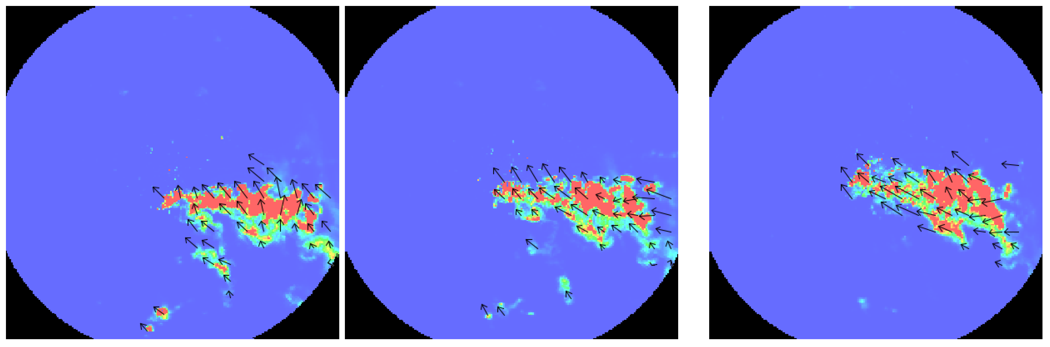
• More comprehensive simulations illustrate the performance of the algorithm in different conditions. Further, the algorithm is applied to simulated GSN sampling data from weather radar images collected during a precipitation event, and the motion estimation performance of the GSN is compared to that of a state-of-the-art image-based optical flow algorithm applied to the weather radar directly, which is a common approach from nowcasting [5]. In this way, the most complete information from the radar images can be compared to the sparse information from the nodes.

The paper is organized as follows: In Section 3, the necessary background knowledge on gradient-based optical flow methods is provided, as well as a compilation of related work. Section 4 provides a description of the methodology for motion estimation with a GSN. In Section 5, the algorithm is evaluated using simulated fields, as well as fields estimated from weather radar. Section 6 provides a concluding discussion on the results and potential limitations of the algorithm, summarizes the main findings and provides an outlook for future extensions.

3. Background and Related Work

3.1. Related Work

There exists a significant amount of work on the estimation of the properties of dynamic spatio-temporal fields with GSN. Problems include the estimation of field boundaries [16], the identification of a critical point, such as peaks and pits [17], or even spatial interpolation in the network [18]. The book of Duckham [11] provides a thorough overview of this topic, as well as a description of the advantages of decentralized computation in the network, which also apply to the work presented in this paper. Another research line related to our work is the tracking (following) of advected spatio-temporal features by mobile nodes [19,20]. While in these works, mobile nodes are assumed that can either move by themselves or move with the field (e.g., buoys moved by ocean currents), our work assumes a network of stationary nodes (or cars whose movement is predetermined by the road network) and aims to estimate the motion from the time series of sensor measurements collected by the nodes. Further, there is a significant amount of work on object tracking with GSNs, i.e., generating information on the trajectory of a mobile object without necessarily following it, such as [21]. However, to the best of our knowledge, the problem of estimating field- (not object-) motion with a GSN has not been tackled so far.

3.2. Network and Field Model

A GSN is modeled as a graph $G=(V,E)$ where V is the set of nodes distributed on the plane and E is the set of communication links between nodes. The allowed bidirectional communication links are solely determined by a maximum Euclidean communication distance r (unit distance) in the plane, and hence, G is a unit disk graph (UDG, [11]). A node $n_i\in V$ knows its position $s_i=(x_i,y_i)$ on the plane, e.g., by using the Global Positioning System (GPS). Further, the nodes are able to sense a real-valued scalar spatio-temporal field $Z\left(u\right):{\mathbb{R}}^2\times \mathbb{R}\to \mathbb{R}$ where $u={[x,y,t]}^T$ is a location in the space-time cube (and ${\left[\right]}^T$ indicates the matrix transposition). A particular sensor measurement of node $n_i$ at time step t is denoted with $z\left(u_{i,t}\right)$ where $u_{i,t}={[x_i,y_i,t]}^T$. Partial derivatives of the field along spatial axes X and Y and temporal axis T at a particular spatio-temporal location u are written as $Z_X^{\prime }\left(u\right)$, $Z_Y^{\prime }\left(u\right)$ and $Z_T^{\prime }\left(u\right)$. Their estimates provided by a node $n_i$ at time t are denoted with ${\widehat{z}}_X^{\prime }\left(u_{i,t}\right)$, ${\widehat{z}}_Y^{\prime }\left(u_{i,t}\right)$ and ${\widehat{z}}_T^{\prime }\left(u_{i,t}\right)$. The column vector of estimated partial derivatives is then written as ${\widehat{z}}^{\prime }\left(u_{i,t}\right)={[{\widehat{z}}_X^{\prime }\left(u_{i,t}\right),{\widehat{z}}_Y^{\prime }\left(u_{i,t}\right),{\widehat{z}}_T^{\prime }\left(u_{i,t}\right)]}^T$.

3.3. Optical Flow: Basics

Optical flow methods, such as [12] or [22], are usually employed for estimating pixel displacement (motion) in between two images. The assumption underlying most optical flow approaches is that the intensity (pixel/field values) remains constant in between the sampling periods and a change in values for a particular location solely comes from field motion. Formally, this means that there exists a vector in the space-time cube $h={[\Delta x,\Delta y,\Delta t]}^T$ such that Equation (1) holds.

$$Z\left(u\right)=Z(u+h)$$

(1)

Optical flow methods can be classified into two categories: those that use partial derivatives in space and time for estimation and those that use matching of image parts (also known as block matching) [10]. Applying the block matching methodologies for irregular data would require interpolation of the irregular data to regular grids, which would introduce additional assumptions about the field structure. Instead, a gradient-based approach is chosen where the partial derivatives are estimated from irregular data using least-squares adjustment. Those gradient-based methods are based on the assumption that a first-order Taylor series expansion of the values is adequate, as displayed in Equation (2).

$$Z(u+h)\cong Z\left(u\right)+Z_X^{\prime }\left(u\right)\Delta x+Z_Y^{\prime }\left(u\right)\Delta y+Z_T^{\prime }\left(u\right)\Delta t$$

(2)

where $Z_X^{\prime }$, $Z_Y^{\prime }$ and $Z_T^{\prime }$ are the partial derivatives in the space-time cube. Equation (2) is called the linearity assumption of optical flow, as higher order terms are ignored. Combining (1) and (2) and dividing by $\Delta t$ then results in the gradient constraint (GC) Equation (3).

$$Z_X^{\prime }\left(u\right)\Delta x/\Delta t+Z_Y^{\prime }\left(u\right)\Delta y/\Delta t+Z_T^{\prime }\left(u\right)\cong 0$$

(3)

Instantiating Equation (3) requires estimates of the partial derivatives. Usually, they are estimated with numerical differentiation using neighboring (in space and time) pixel values. Estimating optical flow $v_X=\Delta x/\Delta t$ and $v_Y=\Delta y/\Delta t$ then requires at least two gradient constraints to be integrated. The linearity assumption of Equation (2) implies that the length of the displacement h has an influence on motion estimation accuracy: the shorter the displacement, the more valid the expansion of Equation (2) and, thus, the more accurate are the motion estimates. There is also an interplay between the degree of linearity of the field and the motion estimation accuracy: for a linear field, Equation (2) holds exactly (≅ can be replaced by =).

4. Methodology

The proposed decentralized algorithm for motion estimation consists of two parts:

• Gradient constraint estimation: Estimates of a gradient constraint at a node $n_i$ at time t, ${\widehat{z}}_X^{\prime }\left(u_{i,t}\right)$, ${\widehat{z}}_Y^{\prime }\left(u_{i,t}\right)$ and ${\widehat{z}}_T^{\prime }\left(u_{i,t}\right)$, are calculated from sensor measurements of neighboring nodes. The error of a GC is derived from the spatial configuration of the node neighborhood. Details are given in Section 4.1.
• Motion estimation: A set of estimates of gradient constraints is integrated at each time step t by each node $n_i$ over its direct 1-hop neighborhood to solve for the motion components. Further details are provided in Section 4.2.

In Appendix A, the algorithm protocol is provided. More details on the involved equations, e.g., the normal equations for solving a least squares problem, are provided in the previous publication on the topic [14].

4.1. Gradient Constraint Estimation

The methodology for gradient-based, decentralized motion estimation with a stationary GSN is described in detail in [14]. In short, the irregular sampling of the data requires the indirect estimation of $Z_X^{\prime }\left(u\right)$, $Z_Y^{\prime }\left(u\right)$ and $Z_T^{\prime }\left(u\right)$ by numerical estimates of directional derivatives calculated from sensor samples that are irregularly distributed in space and time (Equation (4)).

$${\widehat{z}}_{d_{ij,tr}}^{\prime }\left(u_{i,t}\right)=\frac{z\left(u_{j,r}\right)-z\left(u_{i,t}\right)}{|d_{ij,rt}|}$$

(4)

where $d_{ij,tr}$ is the spatio-temporal distance vector between the spatio-temporal node locations $u_{i,t}$ and $u_{j,r}$ (the locations of node i at time t and node j at time r), and $z\left(u_{i,t}\right)$ and $z\left(u_{j,r}\right)$ are field samples at these locations, collected by the nodes. The functional relationship between the estimate of such a directional derivative and the partial derivatives along the space-time cube coordinate axes is displayed in Equation (5) (for easing the readability, the spatio-temporal location index $u_{i,t}$ is omitted in the following equation).

$${\widehat{z}}_d^{\prime }={\widehat{z}}_X^{\prime }{\widehat{u}}_{X,d}+{\widehat{z}}_Y^{\prime }{\widehat{u}}_{Y,d}+{\widehat{z}}_T^{\prime }{\widehat{u}}_{T,d}$$

(5)

where ${\widehat{u}}_{X,d}$, ${\widehat{u}}_{Y,d}$ and ${\widehat{u}}_{T,d}$ are the unit vector components in the particular spatio-temporal direction d, ${\widehat{z}}_d^{\prime }$ is a particular estimate of a directional derivative calculated with Equation (4) and ${\widehat{z}}_X^{\prime }$, ${\widehat{z}}_Y^{\prime }$ and ${\widehat{z}}_T^{\prime }$ are estimates of the partial derivatives required for optical flow. A set of such linear equations available at a specific spatio-temporal node position $u_{i,t}$ then forms a linear system of the form of Equation (6).

$$A\left(u_{i,t}\right){\widehat{z}}^{\prime }\left(u_{i,t}\right)=\widehat{b}\left(u_{i,t}\right)$$

(6)

where $A\left(u_{i,t}\right)$ is the matrix containing the unit vectors as rows, ${\widehat{z}}^{\prime }\left(u_{i,t}\right)={[{\widehat{z}}_X^{\prime }\left(u_{i,t}\right),{\widehat{z}}_Y^{\prime }\left(u_{i,t}\right),{\widehat{z}}_T^{\prime }\left(u_{i,t}\right)]}^T$ is the column vector of partial derivatives to be estimated, i.e., ${\widehat{z}}^{\prime }\left(u_{i,t}\right)$ is an estimate of the gradient constraint of Equation (3). $\widehat{b}\left(u_{i,t}\right)$ is the column vector of estimates of directional derivatives. The system then allows solving for ${\widehat{z}}^{\prime }\left(u_{i,t}\right)$, e.g., by ordinary least squares adjustment (OLS) or weighted least squares adjustment (WLS) with a certain weight matrix W for the observations (more details on the approach, e.g., the normal equations for solving the least squares problem, are provided in [14]).

4.1.1. Stationarity of Nodes

As the distance vector $d_{ij,tr}$ is a vector in space and time, the calculation of the length $|d_{ij,tr}|$ requires the a priori specification of a spatio-temporal anisotropy factor, such as a decision on the unit of measures. If this knowledge is available a priori, the nodes are allowed to move and sample the field asynchronously, i.e., at different time steps. In this work, it is assumed that the anisotropy factor is not known, and the assumptions of node stationarity and time synchronicity are essential (see [14] for a more thorough elaboration on this topic). In this case, space can be treated as separated from time: the linear system only includes spatial derivatives, while the temporal change can be estimated by each node individually from the difference of the current and previous field sample measured by that node: ${\widehat{z}}_T^{\prime }\left(u_{i,t}\right)=z\left(u_{i,t}\right)-z\left(u_{i,t-1}\right)$. With this fixed spatial configuration, the matrix $A\left(u_{i,t}\right)$ in the linear system of Equation (6) is time-independent and constant for each node $n_i$ (it is denoted with $A_i$ in the following) and the normal equations for solving the system can be pre-computed at the initialization phase of the algorithm (Appendix A). It is clear that this assumption does not hold for non-stationary, moving nodes, e.g., cars. Nonetheless, in Section 5, the algorithm is applied in a non-stationary setting with simulated cars, with only slight modifications detailed in Appendix A.

4.1.2. Error in Derivative Calculation

As, due to node stationarity, the change along the time axis can be directly estimated by each node by backward differencing, no error for the estimated temporal derivative ${\widehat{z}}_T^{\prime }\left(u_{i,t}\right)$ is assumed. For estimating the error (and therefore, the weights in the WLS adjustment) associated with the estimate of a particular directional derivative in space, the heuristic displayed in Equation (7) is used:

$${ϵ}_{ij}=\frac{d_{ij}}{r}$$

(7)

where r is the maximum possible communication range in between the nodes and $d_{ij}$ is spatial distance between the two nodes $n_i$ and $n_j$. The weight matrix $W_i$ in the WLS adjustment then contains the inverse of ${ϵ}_{ij}$ as the weight on the diagonal and zeros elsewhere, as no dependency between the observations is assumed. Due to stationarity of nodes, $W_i$ is constant for each node and can be precomputed. From the definition of directional derivatives provided in [14], it is clear that the closer two measurements are, the better the numerical differentiation of Equation (4) approximates the true directional derivative. This particular weight accounts for this by down-weighting measurements with increasing spatial distance from the estimating node. Dividing distance by communication range ensures that the down-weighting is significant and independent of the unit of measure of spatial distance. The usefulness of this weighting compared to a uniform weighting is shown in the evaluation provided in Section 5.4.3. The error associated with the derived partial derivatives can then be estimated from individual directional derivative errors using the law of propagation of error (see, e.g., [23,24] or any geodetic textbook):

$$C_{G{C}_i}={\left(A_i^T{W}_i{A}_i\right)}^{-1}$$

(8)

where $C_{G{C}_i}$ is the $2\times 2$ so-called cofactor matrix of the $2\times 1$ vector of estimated spatial partial derivatives ${\widehat{z}}^{\prime }\left(u_{i,t}\right)={[{\widehat{z}}_X^{\prime }\left(u_{i,t}\right),{\widehat{z}}_Y^{\prime }\left(u_{i,t}\right)]}^T$. Since the nodes are assumed to be stationary, matrix $A_i$ and weight matrix $W_i$ are constant and hence $C_{G{C}_i}$ is constant for a particular node $n_i$ and can be pre-computed as well (Appendix A). Since field properties have been ignored in Equation (8), $C_{G{C}_i}$ is not a proper covariance matrix, and the diagonal entries of $C_{G{C}_i}$ are not absolute, but only relative representations of the errors of the estimated partial derivatives ${\widehat{z}}_X^{\prime }\left(u_{i,t}\right)$ and ${\widehat{z}}_Y^{\prime }\left(u_{i,t}\right)$ estimated by that node ([24]). Therefore, in order to derive a valid covariance matrix for each ${\widehat{z}}^{\prime }\left(u_{i,t}\right)$ provided by node $n_i$, the entries of $C_{G{C}_i}$ have to be transformed to the proper level of error for the specific field under consideration and for the specific time step t. A common approach in least squares adjustment is to derive a so-called variance-factor from the least squares adjustment and to multiply it with $C_{G{C}_i}$ to derive the empirical covariance matrix for the estimated partial derivatives ${\widehat{z}}^{\prime }\left(u_{i,t}\right)$ at node $n_i$ at time t:

$${\Sigma }_{{\widehat{z}}^{\prime }}\left(u_{i,t}\right)={\widehat{\sigma }}^2\left(u_{i,t}\right)C_{G{C}_i}$$

(9)

The required variance factor ${\widehat{\sigma }}^2\left(u_{i,t}\right)$ can be calculated with:

$${\widehat{\sigma }}^2\left(u_{i,t}\right)=\frac{v{\left(u_{i,t}\right)}^T{W}_{i}v\left(u_{i,t}\right)}{f}$$

(10)

where $v\left(u_{i,t}\right)$ is the column vector of deviations of the least squares adjustment for node $n_i$ at time t (i.e., it contains the result of ${\widehat{z}}_X^{\prime }{\widehat{u}}_{X,d}+{\widehat{z}}_Y^{\prime }{\widehat{u}}_{Y,d}-{\widehat{z}}_d^{\prime }$ as row entries for each directional derivative/neighboring node at time t). $f=m-p$ is the degrees-of-freedom with m being the number of neighbors of a node and p the number of parameters ($p=2$ for the stationary case). Calculating the variance factor is a common approach in least squares adjustment, e.g., for GPS positioning [23], in order to quantify the error of the derived parameters/coefficients; in this case, the error of the least squares result ${\widehat{z}}^{\prime }\left(u_{i,t}\right)$. However, calculating a stable ${\widehat{\sigma }}^2\left(u_{i,t}\right)$ at each time step t usually requires sufficient degrees-of-freedom in the order of p to $2p$ [24]. Thus, for a sufficiently large f, a node is required to have 4 to 6 (resp. 6 to 9) neighbors. Therefore, an a priori variance factor is used in the following, equal to all nodes and denoted with ${\widehat{\sigma }}^2$, which is, however, derived from observed values for ${\widehat{\sigma }}^2\left(u_{i,t}\right)$. A particular advantage of using a pre-calculated variance factor is that in a stationary setting, the variance factor ${\widehat{\sigma }}^2\left(u_{i,t}\right)$ for a node $n_i$ is constant and therefore, the covariance matrix of the partial derivative calculated by the node ${\Sigma }_{{\widehat{z}}^{\prime }}\left(u_{i,t}\right)$ is constant as well (written as ${\Sigma }_{{\widehat{z}}^{\prime },i}$ in the following) and can be pre-computed (see Appendix A or [14] for more details).

4.1.3. Gradient Constraint Error Estimation

The motion estimation methodology described in Section 4.2 requires an estimate of the error associated with a particular estimate of a GC, ${\widehat{z}}^{\prime }\left(u_{i,t}\right)$, in the form of a scalar error variance. In order to derive such a measure for a GC, the probabilistic approach of [25] is used, who derives a probability distribution for the motion components from the gradient constraint. The gradient constraint of Equation (3) is an idealization for several reasons [25]: the true spatial and temporal derivatives are not available, but their estimates are. Further, the gradient constraint is a constraint on the (optical) flow and not on the true motion of the field. For example, when using gradient constraints for estimating the motion of a precipitation field, the motion can be determined only at locations where there is some precipitation. In those regions where there is no rainfall, the motion estimate will be zero, as the spatial and temporal derivatives are zero, although there might still be motion in the atmosphere. Since the optical flow gradient constraints are usually integrated in space, a spatial neighborhood that includes rainfall and no rainfall will exhibits different “optical motions” and, therefore, provides an averaged motion estimate (see also Section 1.2 of [25], where this is called the “blank-wall” problem). Therefore, [26] introduced a probabilistic model for the gradient constraint (further details can be found in the doctoral thesis [25]) including three possible sources of error, each characterized by Gaussian random noise variables. Here, the model of [25]) is used, but it is assumed that the estimation of the partial derivatives in space is the dominant source of error and that there is no error in the estimated temporal derivative. Further, the error relating to the difference in between the “optical flow” and the true motion is considered by neglecting GCs in the estimation process, when at least one of the following conditions applies:

• Zero-field values: When the field values used for derivative calculation are zero and, hence, all derivatives are zero, the GC is not estimated at all. Usually, measurements of spatio-temporal fields are zero-inflated, meaning that the majority of samples are zero. In such a case, no motion can be estimated, and node energy can be saved.
• Node neighborhood extending field boundary: When only one of the sensor samples for estimating the GC is zero, the GC is not estimated at all, as the node neighborhood extends over the field boundaries. While the GC could still be estimated using the remaining sensor samples, this is not done, as the least squares matrices for estimating the partial derivatives are pre-computed (see [14] for the details).
• Non-zero, but equal field values: When the field is completely flat, corresponding to the “blank wall” problem described previously, the GC is not estimated at all. This case can be recognized, when all of the neighboring sensor samples of a timestep t are larger than zero, but equal. Then, the derivatives are zero, and the GC does not contribute to the motion estimation.

For deriving a gradient constraint error measure when none of the above cases applies, the approach of [25] is used: it is assumed that the true spatial derivatives are related to the estimated spatial derivatives via some random noise variables $n_{z_X}$ and $n_{z_Y}$ (again, the spatio-temporal location parameter $u_{i,t}$ is skipped for easing readability).

$$\begin{array}{cc}\hfill {\widehat{z}}_X^{\prime }& =Z_X^{\prime }+n_{z_X^{\prime }}\hfill \\ \hfill {\widehat{z}}_Y^{\prime }& =Z_Y^{\prime }+n_{z_Y^{\prime }}\hfill \end{array}$$

where ${\widehat{z}}_X^{\prime }$ and ${\widehat{z}}_Y^{\prime }$ are the estimated partial derivatives in X and Y direction, $Z_X^{\prime }$ and $Z_Y^{\prime }$ are the true derivatives and $n_{z_X^{\prime }}$ and $n_{z_Y^{\prime }}$ are the noise variables. Since no error for the estimate of the temporal derivative is assumed, a GC (Equation (3)) can be reformulated as follows:

$$\begin{array}{cc}\hfill 0& =Z_X^{\prime }{v}_X+Z_Y^{\prime }{v}_Y+Z_T\hfill \\ & =({\widehat{z}}_X^{\prime }-n_{z_X^{\prime }})v_X+({\widehat{z}}_Y^{\prime }-n_{z_Y^{\prime }})v_Y+{\widehat{z}}_T^{\prime }\hfill \\ & ={\widehat{z}}_X^{\prime }{v}_X-n_{z_X^{\prime }}{v}_X+{\widehat{z}}_Y^{\prime }{v}_Y-n_{z_Y^{\prime }}{v}_Y+{\widehat{z}}_T^{\prime }\hfill \end{array}$$

From this, the probabilistic relationship between the estimates of the partial derivatives and the true motion that is to be estimated can be derived [25]:

$$\Rightarrow {\widehat{z}}_X^{\prime }{v}_X+{\widehat{z}}_Y^{\prime }{v}_Y+{\widehat{z}}_T^{\prime }=n_{z_X^{\prime }}{v}_X+n_{z_Y^{\prime }}{v}_Y$$

(11)

Under the assumption of zero-mean independent Gaussian noises, the right-hand term of Equation (11) is a zero-mean random variable with variance:

$${\sigma }_{GC}^2={\sigma }_{z_X^{\prime }}^2{v}_X^2+{\sigma }_{z_Y^{\prime }}^2{v}_Y^2$$

(12)

where ${\sigma }_{z_X^{\prime }}^2$ and ${\sigma }_{z_Y^{\prime }}^2$ are the variances of $n_{z_X^{\prime }}$ and $n_{z_Y^{\prime }}$, resp., and $v_X$ and $v_Y$ are the field motions. The statistical independence of $n_{z_X^{\prime }}$ and $n_{z_Y^{\prime }}$ cannot be expected to hold in reality, but as no information on the dependence (i.e., covariance) can be made, this is a necessary simplification. The relationship of Equation (12) makes sense, as a gradient constraint can be understood as a regression equation without intercept, the coefficients $v_X$ and $v_Y$, the independent variables $-Z_X^{\prime }$ and $-Z_Y^{\prime }$ and the dependent variable $Z_T^{\prime }$ (this is also the Kalman filter formalization described in the next section). The tuples $({\widehat{z}}_X^{\prime },{\widehat{z}}_Y^{\prime },{\widehat{z}}_T^{\prime })$ are used for calibrating the coefficients. Then, it is clear that the smaller the regression coefficients $v_X$ and $v_Y$, the smaller the influence of ${\sigma }_{z_X^{\prime }}^2$ and ${\sigma }_{z_Y^{\prime }}^2$, disappearing completely for a flat regression plane, i.e., $v_X=v_Y=0$. The terms ${\sigma }_{z_X^{\prime }}^2$ and ${\sigma }_{z_Y^{\prime }}^2$ in Equation (12) can be derived from the covariance matrix of the vector of partial derivatives (the diagonal entries of ${\Sigma }_{{\widehat{Z}}^{\prime }}$ of Equation (9)). The terms $v_X$ and $v_Y$ are unknown and have to be predefined and are therefore a parameter of the algorithm. In this case, the assumed error of a gradient constraint provided by a node $n_i$ is constant and solely determined by spatial configuration. Therefore, it can be precomputed at the initialization phase of the algorithm (Appendix A) and is denoted with ${\sigma }_{G{C}_i}^2$ in the following. In case of negative $n_{z_X^{\prime }}$ and $n_{z_Y^{\prime }}$, the estimated spatial derivatives are underestimates of the true spatial derivatives. Then, the motion estimates will overestimate the true motion speed. This can be explained by means of a simple example: with a fixed temporal absolute derivative and low absolute spatial derivatives, the field must move a larger distance in space in order to render the GC equation valid, i.e., the absolute values of $v_X$ and $v_Y$ must be larger. Conversely, larger absolute spatial derivatives result in smaller speed.

4.2. Temporal Coherence: Kalman Filter for Motion Estimation

The problem of estimating motion from a set of GCs can be considered as a multivariate, intercept-free linear regression model with the motion components in both directions as the model parameters/coefficients, the spatial partial derivatives as the regressors (i.e., independent variables) and the partial derivative in time as the response (i.e., dependent) variable (Equation (13)):

$$Z_T^{\prime }=-Z_X^{\prime }{v}_X-Z_Y^{\prime }{v}_Y$$

(13)

However, the model differs from classical multivariate regression problems in that the response variable is assumed to be error-free, while the regressors are subject to error (see Section 4.1.3). Therefore, estimation methods accounting for these errors in the data would be required (i.e., errors-in-variables regression models, such as total least squares). However, we leave the investigation of such estimation methods to future work and use standard ordinary least squares (OLS) for solving the model. For calibration with GCs collected over space and time, a decision is required on which GCs are integrated to estimate motion at a particular node $n_i$ and time step t. Here, it is assumed that within the one-hop node neighborhood, the motion is uniform. Therefore, a node integrates the GCs provided by its direct neighbors. For integrating GCs in time, a recursive least-squares estimation method is used in the form of a Kalman filter [13] (see also [27] for an application of Kalman filtering to regression problems). The Kalman filter has several advantages over least-squares methods for time series data, as it does not require the storage of large amounts of past data, reduces the computational costs when updating the regression coefficients and comes in a predict-and-update formalization that fits well to the problem. The Kalman filter requires an initial decision on the state variables. The most simple form for the problem at hand is a Kalman state with only the two motion components, which has been used in [14]. In this case, motion is considered constant, and motion change is solely modeled by setting the prediction error variance Q larger than zero. Including motion change variables (i.e., first derivatives of motion with respect to time) into the Kalman state is slightly more realistic by assuming motion change constancy. The Kalman state $v_i\left(k\right)$ including motion derivatives at a node i and time step k is:

$$v_i\left(k\right)=\left[\begin{array}{c}{v}_X\\ v_Y\\ {\dot{v}}_X\\ {\dot{v}}_Y\end{array}\right]$$

(14)

where $v_X$ and $v_Y$ are the motion vector components in the directions X and Y, resp. ${\dot{v}}_X$ and ${\dot{v}}_Y$ are the motion derivatives, i.e., acceleration. The prediction matrix F is:

$$F=\left[\begin{array}{cccc}1& 0& \Delta t& 0\\ 0& 1& 0& \Delta t\\ 0& 0& 1& 0\\ 0& 0& 0& 1\end{array}\right]$$

(15)

where $\Delta t=k-(k-1)$, i.e., the difference in between filter steps. In order to use the Kalman measurement equation for updating the motion state with a new gradient constraint instance, the gradient constraint of Equation (3) is recast into the linear regression form of Equation (13) (see [27] or [28] for the theory on Kalman filtering for linear regression problems with time series data). Then, the temporal derivative $Z_{i,T}^{\prime }\left(k\right)$ is considered a linear function of the motion components and the partial derivatives in space. The Kalman filter measurement matrix is time and node dependent and contains the current partial derivatives (Equation (16)).

$$H_i\left(k\right)=\left[\begin{array}{cccc}-Z_{i,X}^{\prime }\left(k\right)& -Z_{i,Y}^{\prime }\left(k\right)& 0& 0\end{array}\right]$$

(16)

This way, the motion state of a single node $n_i$ is updated with new GCs. Since the measurement $Z_{i,T}^{\prime }\left(k\right)$ is scalar, the measurement error variance R is scalar, and therefore, solving the Kalman update equations does not require matrix inversion [27], which is advantageous for the amount of processing required. The specification of an a priori state is required, which can only be set to the zero vector. The a priori uncertainty, the initial P, should contain large values on the diagonal, indicating the low confidence in the initial state. The uncertainty associated with prediction Q depends on the temporal sampling rate, i.e., the time difference between Kalman filter steps, as well as the assumed motion and motion change constancy of the spatio-temporal field. Therefore, domain knowledge could be employed for setting the required variances. For example, when sampling an atmospheric field, such as precipitation at a sampling rate of 1 min, the difference in motion in between adjacent 1-min time steps can be expected to be in a very low km/h range. The scalar measurement noise variance R is a direct function of GC accuracy. Further, it depends on the spatial distance between the node estimating the motion and the node estimating the GC. The assumption is: the closer the two nodes are, the more similar is the motion. In addition, as described in work on image-based optical flow, such as [12], the GC accuracy depends on field properties at the site where it is constructed. However, in this work, the main source of error is considered to be the partial derivative error, and therefore, the measurement noise variance R is calculated using Equation (12) with a pre-computed variance factor. The presented Kalman filter model is considered generic enough for capturing the field motion behaviors that occur, and it encompasses the constant motion model of [14] by setting the initial motion change variables and the initial motion change error variance to zero.

5. Empirical Evaluation

In this section, the algorithm performance is evaluated empirically for a simulated field (Section 5.4) and a precipitation field derived from weather radar (Section 5.5).

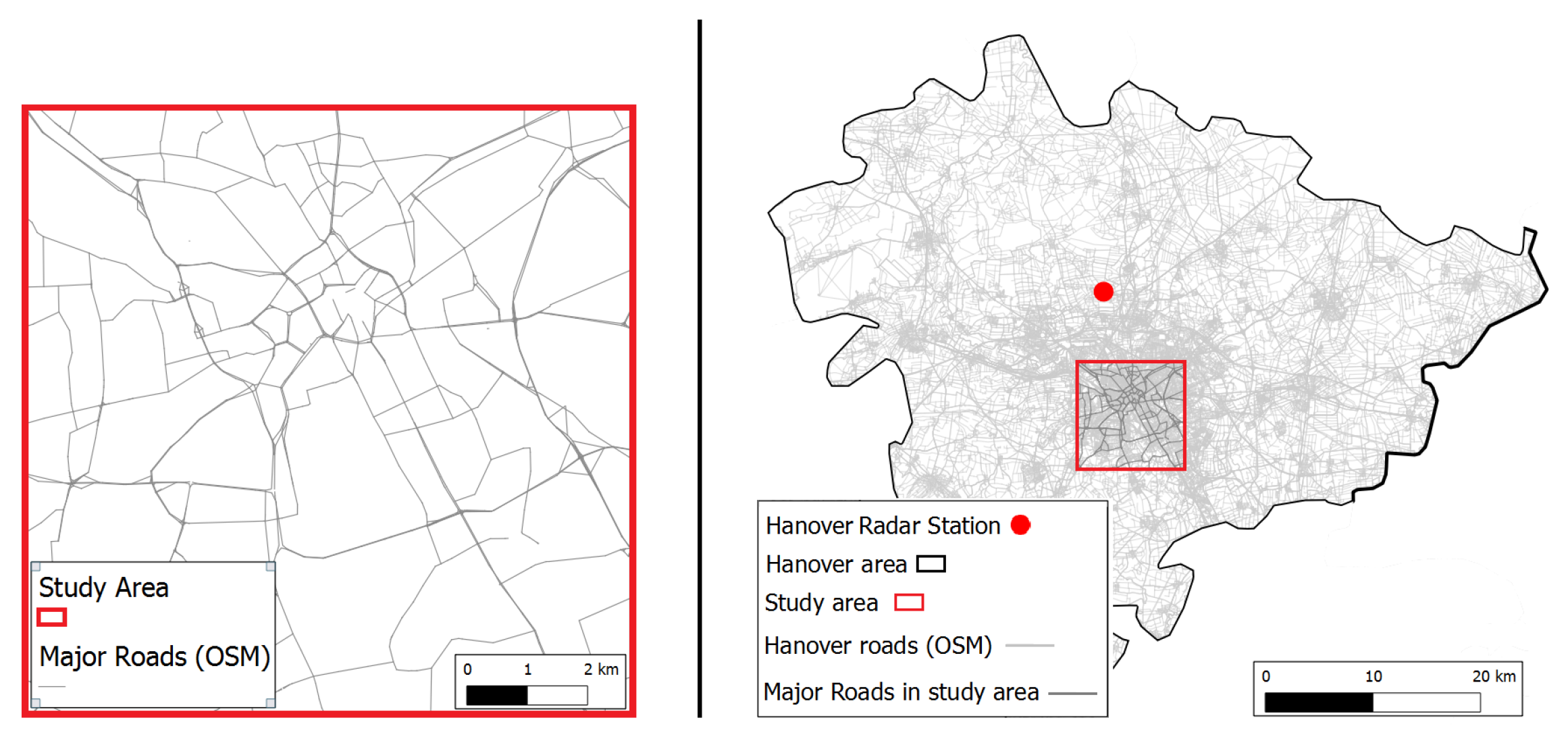
5.1. Study Area, Sensor Network and Deployment Strategy

A 10 km × 10 km area in the center of Hanover city is chosen as the study area for evaluating the proposed motion estimation algorithm (Figure 2).

This particular study area has been chosen due to the availability of weather radar data. The weather radar covers a much larger area, but current GSN technology usually restricts communication distances to ranges of tens to hundreds of meters, in order to reduce energy demand. Therefore, in order to account for the low communication ranges, a small urban sub-area of the radar-covered area is chosen. When cars are used as GSN, it can be expected that the accuracy decreases for areas with lower road density, e.g., rural areas.

A GSN with a UDG communication model is simulated, and different deployment strategies are tested (Figure 3). First, nodes are distributed in the study area in a completely random way (Figure 3a), usually resulting in a disconnected graph where only a subset of nodes is able to estimate motion. Second, a regular grid-based deployment is tested (Figure 3b). Then, as two more realistic cases, a diffusion-based deployment is simulated based on a source node in the center of the study area, for example a base station or node collecting the results (termed sink [11]), where the density is controlled by two parameters, the maximum and minimum distance to neighboring nodes (Figure 3c). In addition, cars are generated on a road network derived from Open Street Map (OSM). The cars move according to a random walk model on the road network with a certain speed, which varies throughout the experiments.

Throughout the experiments, two different node densities and communication ranges are simulated: (1) a low-density, large-distance communication deployment with $n=25$ nodes and a communication range of $r=2000$ m; and (2) a high-density, short-distance communication deployment with $n=400$ and $r=500$ m.

5.2. Error Measures

Following [15], the error of the motion estimation algorithms is quantified using the angular difference between true motion V and estimated motion $\widehat{V}$:

$${ϵ}_{angle}\equiv arccos\left(\frac{\widehat{V}\left(u_{i,t}\right)}{‖\widehat{V}\left(u_{i,t}\right)‖}·\frac{V\left(u_{i,t}\right)}{‖V\left(u_{i,t}\right)‖}\right)\in [0,180]$$

(17)

where ‖‖ is the vector norm, · is the dot-product, $V\left(u_{i,t}\right)={(v_X,v_Y)}^T$ is the true motion at the spatio-temporal node location $u_{i,t}$ and $\widehat{V}\left(u_{i,t}\right)={({\widehat{v}}_X,{\widehat{v}}_Y)}^T$ is the estimated motion, i.e., the Kalman filter state of node i at time t (excluding the acceleration variables). In addition, the difference in motion speed (called “speed offset” in the following) is calculated:

$${ϵ}_{speed}\equiv ‖\widehat{V}\left(u_{i,t}\right)‖-‖V\left(u_{i,t}\right)‖$$

(18)

In the case of a simulated field, the true field motion is known, as it is a parameter of the simulation. For weather radar fields, the motion estimated by the algorithm of [3] is used as true motion, which is estimated from the weather radar images.

5.3. Setting the Filter Parameters

The Kalman filter requires two parameters: the prediction noise and the measurement noise. As in any Kalman filtering problem, if the measurement noise is large compared to the prediction noise, the filter will only slowly follow the measurements and “trust” the predictions more. Here, the individual measurements (gradient constraints) are considered to be rather inaccurate. Therefore, the Kalman measurement noise is significantly larger than the prediction noise, especially as multiple filter updates per time step occur and the motion is assumed to be rather constant over sampling periods. Therefore, and since only constant motion is simulated in the following evaluations, the prediction noise Q is set to the zero matrix in the following evaluations, i.e. $Q=0_{4,4}$. If not indicated otherwise, the scalar measurement noise of the Kalman filter is calculated with Equation (12). The required variance factor is estimated by pre-running the filter and observing the value calculated by Equation (10) for each node. The average variance factor is then used in the simulations. The motion speed parameter required in Equation (12) is set to the maximum possible motion, a parameter that is assumed to be derived from domain knowledge, e.g., knowledge on the maximum possible speed of wind or ocean currents. The initial state of the filter is set to the zero vector; the initial state covariance P is set to large values indicating the uncertainty in the initial state.

5.4. Results: Simulated Field

Simulating realistic atmospheric or oceanographic fields is a complex task. Therefore, the approach taken here is to simulate a rather simplistic spatio-temporal moving field in order to illustrate the basic properties of the proposed algorithm, such as the behavior under different motion speeds. The simulated field is a Gaussian mixture model simulated on a square eight times the size of the original study area (Equation (19)).

$$Z(x,y)=\sum _{i=1}^{n_G}{e}^{-\frac{{(x-{\mu }_{i,x})}^2+{(y-{\mu }_{i,y})}^2}{2{\sigma }_i^2}}$$

(19)

where $n_G$ is the number of Gaussians, ${\mu }_{i,x}$ is the x-coordinate, ${\mu }_{i,y}$ is the y-coordinate of the center of Gaussian i, which are drawn randomly from the coordinate space of the study area. ${\sigma }_i^2$ is the variance, which is drawn randomly from the interval $[0,{\sigma }_{max}^2]$ for each Gaussian. In reality, the fields can be expected to exhibit large parts of zero field values, e.g., periods of no rainfall in between rain clouds. In order to reflect this in the simulations, a minimum possible field value is assumed, and the field is set to zero, if the simulated values fall below this threshold. Due to the linearity assumption of optical flow of Equation (2) and the methodology for derivative estimation, the motion estimation works well when the field is approximately linear at the sites where the gradient constraints are constructed, and the reachable accuracy depends largely on the degree of field linearity. Therefore, two different fields are simulated that differ in their degree of linearity: the more linear one is simulated using a low number of Gaussians with a large maximum variance ${\sigma }_{max}^2$. A more diverse, non-homogenous field is simulated using a high number of Gaussians with a small maximum variance ${\sigma }_{max}^2$. Examples of the resulting fields are displayed in Figure 4a,b.

Different motion behaviors of the field can be simulated by moving the center coordinates of the Gaussians (${\mu }_{i,x}$ and ${\mu }_{i,y}$) through the study area. In order to be able to simulate an unlimited number of time steps, a Gaussian that leaves the area to the west re-appears to the right, etc. The motion behaviors can be distinguished along the properties of motion behavior in time (coherence) and motion behavior in space (uniformity). As the approach assumes local translational motion within the node neighborhood, the motion estimation accuracy certainly depends on the degree of spatial uniformity of motion. Here, it is assumed that the motion is rather homogeneous throughout the node neighborhood, for example rain field motion within a neighborhood of 2000 m, and no evaluation concerning spatial non-uniformity is provided. The motion estimation accuracy certainly also depends on the temporal coherence of motion. Again, although the models allow for changing motion, it is assumed that the motion is rather constant over the period of interest. For investigating the performance of the algorithm, 100 time steps of a constantly- and uniformly-moving field are simulated, and the errors are aggregated for each time step. The visualization displayed in Figure 4 shows a single snapshot of the simulations.

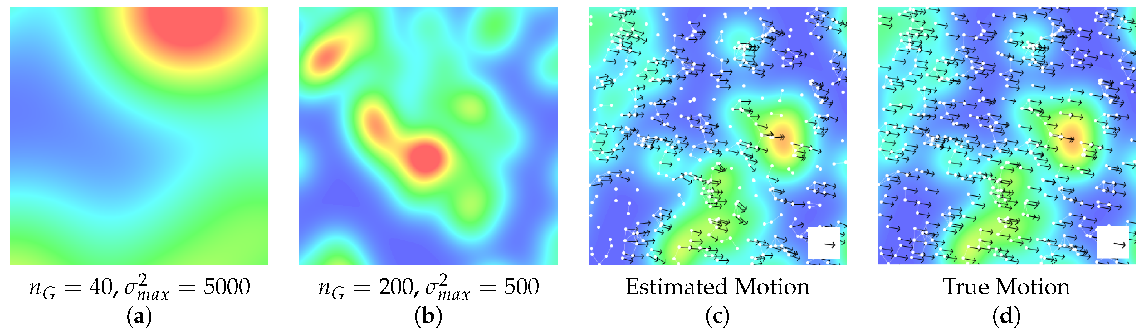
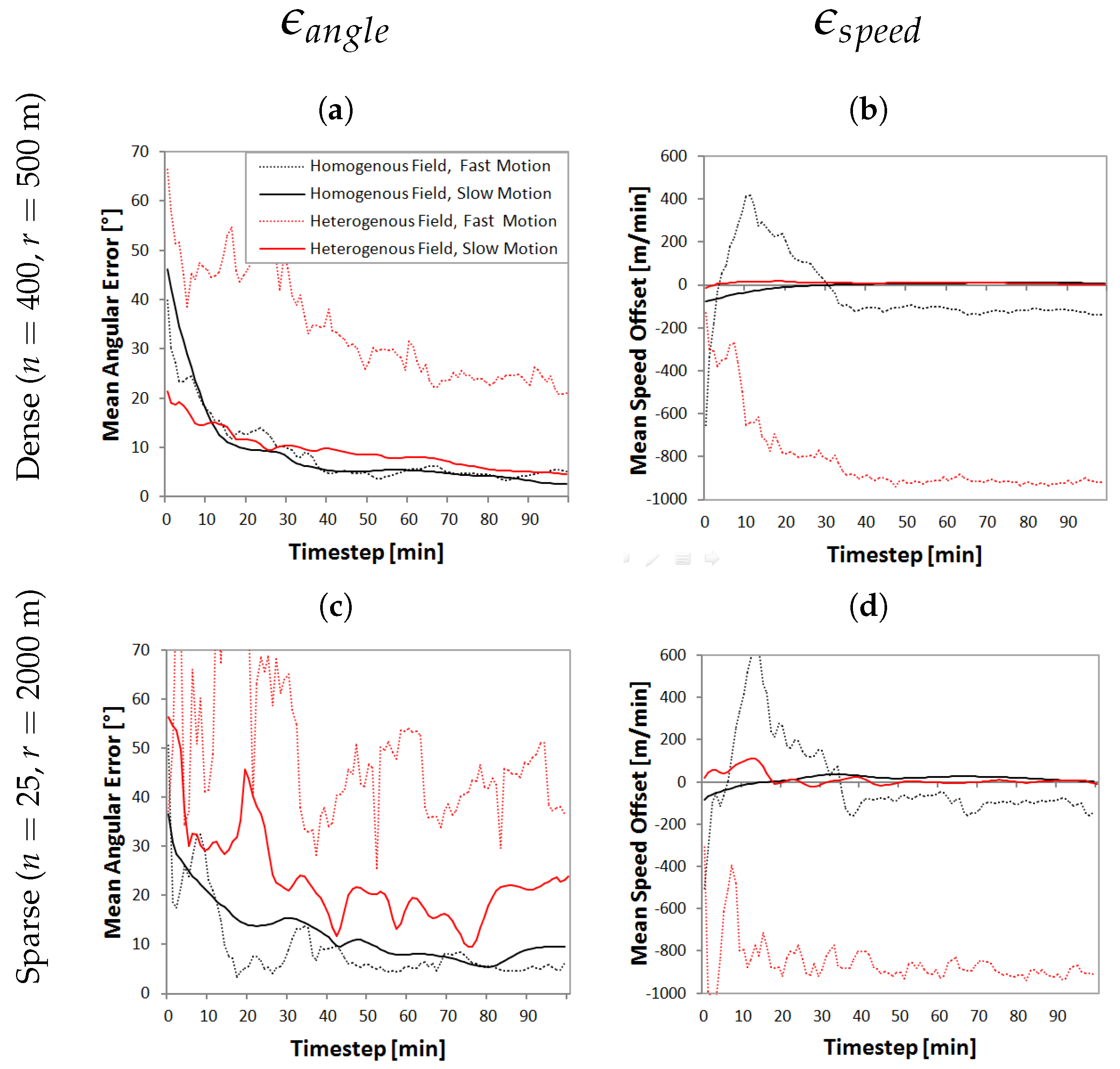
5.4.1. Influence of Field Linearity, Field Speed and Node Density

In the first experiment, the influence of the field, the motion speed and the node density is investigated. In Figure 5, the motion estimation error is displayed as a function of time for two different spatio-temporal fields and the two different motion speeds: fast motion ($v_x=-1000$ m/min and $v_y=1000$ m/min) and slow motion ($v_x=-100$ m/min and $v_y=100$ m/min), as well as the two node network densities in a random node deployment and different UDG communication ranges r.

Over time, the motion estimation error for angle and speed decreases. The more homogeneous (and therefore, linear) the field, the lower the angular error. Further, the motion speed is important: the larger the speed, the less valid the linearity assumption of Equation (2). Both influences, field linearity and motion speed, are strongly related: the more homogeneous and linear the field, the less influential is the motion speed on the estimation accuracy. With a strong non-linearity in field values and large motion, the errors concerning angle and speed get large. The underestimation of speed for large motions is due to the increased invalidity of the Taylor expansion of Equation (2) for large motion vectors. Then, the estimated spatial derivatives seem to overestimate the change in field values for the length of the displacement (see also the last paragraph of Section 4.1.3 for a more detailed elaboration on this topic). Further, the more sparse the deployment, the larger the errors. Therefore, a dense deployment with nodes sampling the field at a high sampling rate is advantageous for motion estimation.

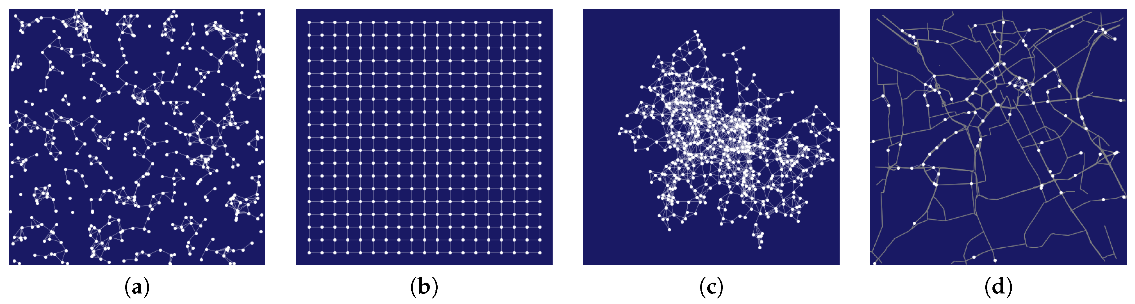
5.4.2. Influence of Deployment Strategy

For evaluating the influence of node deployment on motion estimation results, a homogeneous field is simulated moving slowly over the study area and a dense node deployment. The performance of different deployment strategies introduced previously is tested (Figure 6).

The results show that the approach is rather agnostic of the deployment of stationary nodes. Although, as expected, a grid-based deployment is slightly advantageous, the difference is not considered significant, at least for high numbers of nodes. Motion estimation with a VANET results in significantly larger errors, potentially due to the increased invalidity of the estimate of the temporal derivative. Surprisingly, stationary cars provide large errors, as well, although they are similar to a random deployment of stationary nodes. This can be explained by the spatial configuration and the sampling on the road network: due to the communication range of $r=500$ m, cars usually communicate only when driving on the same road. Therefore, the samples for derivative estimation are often aligned linearly along the road, which is disadvantageous for motion estimation. This is a problem that is very likely to occur in reality, as well.

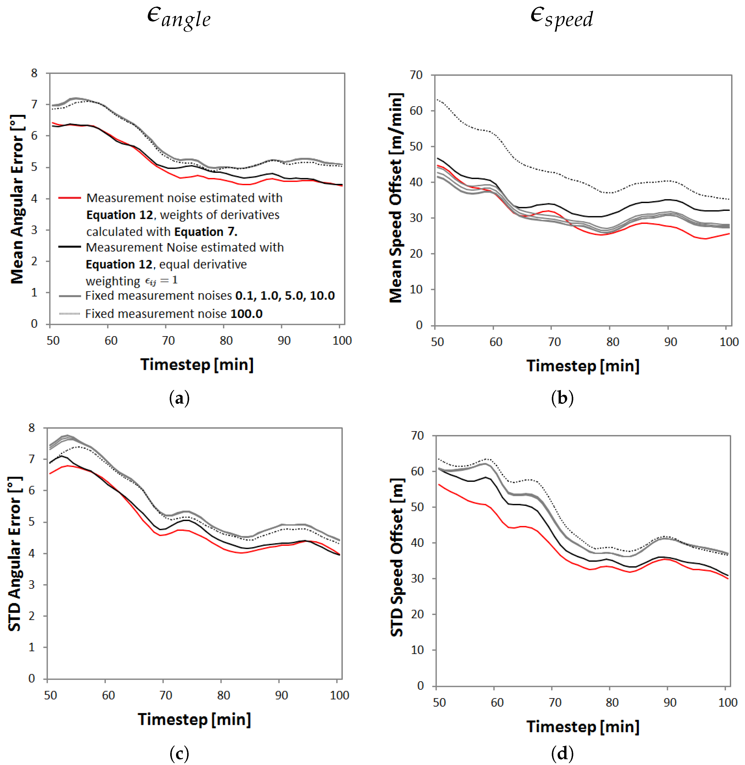
5.4.3. Influence of Kalman Measurement Noise

For investigating the Kalman measurement noise parameter, a GSN of $n=25$ nodes with a UDG communication distance of $r=2000$ m is simulated. The nodes are distributed according to a diffusion-based deployment with a minimum allowed node distance of 1000 m and a maximum node distance equal to the UDG communication range $r=2000$ m. The field motion behavior is randomly chosen from the small interval $v_X\in [-500m/t,500m/t]$ and $v_Y\in [-500m/t,500m/t]$. Different fixed Kalman measurement noises are tested, with an equal weighting of the directional derivatives (i.e., ${ϵ}_{ij}=1$ in Equation (7) for all pairs of nodes). Further, the Kalman measurement noise estimated with the methodology described in Section 4.1.3 is tested. In order to quantify the terms of Equation (12), maximum possible field motions $v_X=1000$ and $v_Y=1000$ are assumed. As described previously, the required variance factor is estimated by pre-running the simulations and calculating an average variance factor using Equation (10). The results presented in Figure 7 are averages of ten runs of simulations with a different spatio-temporal field, different motion and different network each time.

The derivation of gradient constraint errors from spatial configuration seems to be beneficial for motion estimation. Further, the provided formula for deriving the gradient constraint error (Equation (12)) gives a straight-forward way of calculating the required Kalman measurement noise parameter. Without it, the specification of the measurement noise has to rely on rather arbitrary considerations. It can be seen that the estimation accuracy is rather agnostic of a fixed Kalman measurement noise, except for very large noises. The weighting of the directional derivatives seems to provide a slight advantage over a uniform weighting. The speed is overestimated on average because of a general underestimation of the derivatives (see also Section 4.1.3 for a more detailed elaboration on this topic).

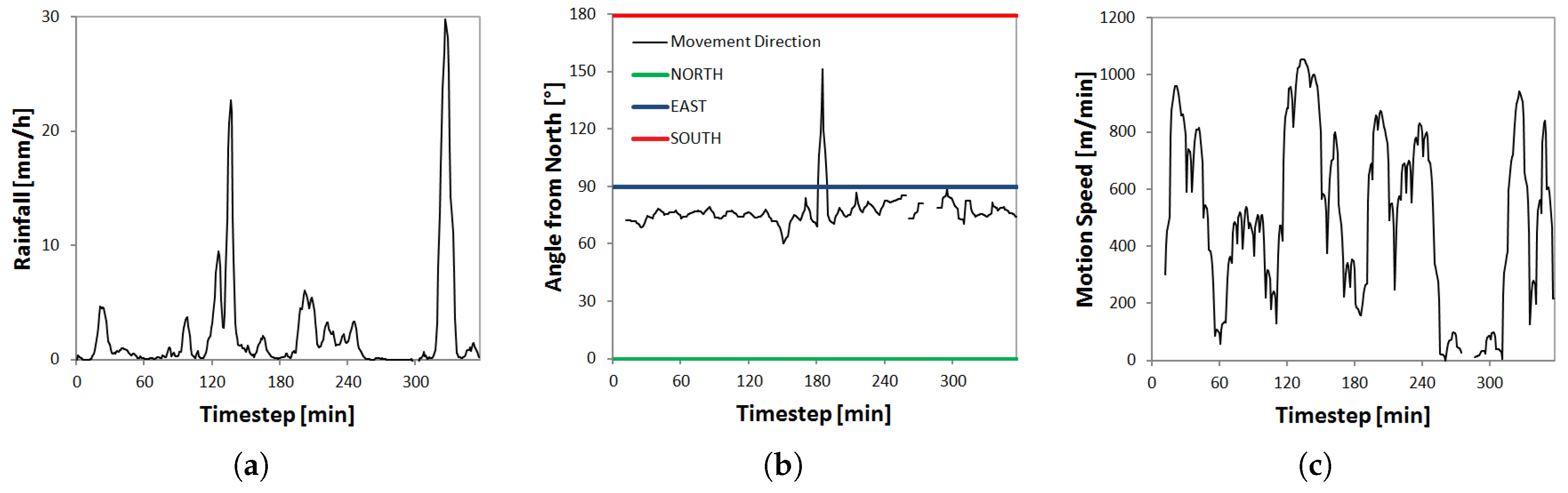
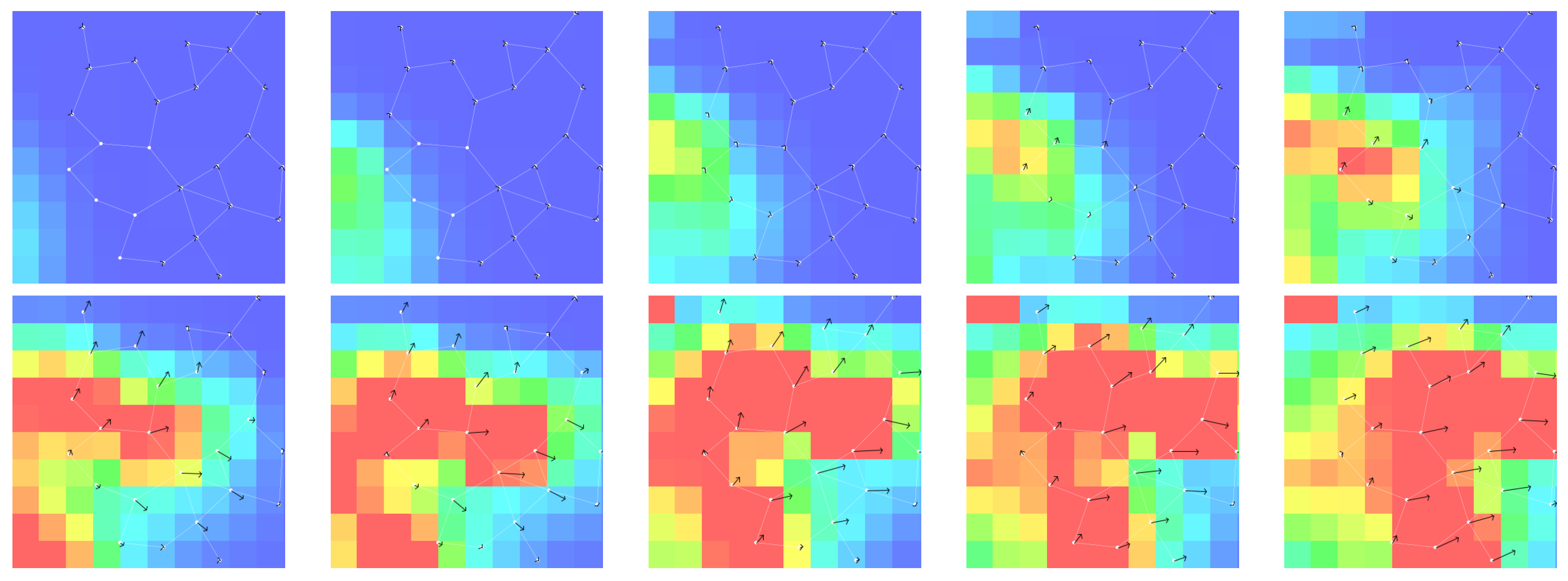
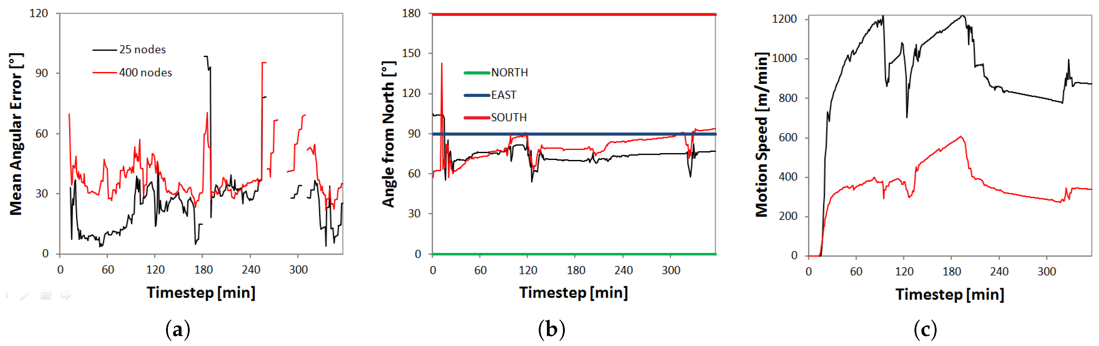
5.5. Results: Radar Field

In a second experiment, the algorithm is evaluated on a precipitation field derived from the Hanover weather radar. Six hours of a period of rather strong rainfall (19 July 2012, 4 a.m. to 10 a.m.) is chosen. The raw radar data (i.e., reflectivities) were preprocessed by using the methodology described in [29], resulting in precipitation values in the unit mm/h on a regular grid with a resolution of 1 ${\mathrm{km}}^2\times$ 1 ${\mathrm{km}}^2$ ($10\times 10$ pixels in the study area) at a sampling rate of 5 min. The radar data are upsampled to 1 min snapshots by using an optical flow algorithm (OpenCV implementation of the algorithm provided by [3]). Further, the resulting grids are smoothed by a $3\times 3$ arithmetic mean filter. As ground truth motion, the flow field derived from the image-based optical flow algorithm is used, which is executed on the whole radar image. An average motion vector per time step is then derived by averaging the vectors over all 10 × 10 pixels of the study area at each 1-min time step. A characterization of the event and the derived motion information is displayed in Figure 8.

Figure 8a shows that a number of rain clouds passes the study area within the six hours, with two very strong rainfall periods. The field moves with a rather constant motion from west to (slightly north) east (a sudden change of direction in the middle of the period occurs, which is potentially due to radar clutter). The motion speed is at around 1000 m per minute, but decreases for periods of low rainfall, which is an artifact of the optical flow algorithm. In Figure 9, time series of 1-min radar snapshots and motion vectors estimated with the proposed algorithm are displayed.

Before the first cloud reaches the study area, no motion estimation is possible. Over time, the motion vectors of the nodes approach the cloud motion direction of east-north-east. For evaluating the performance of the algorithm, the two network densities are simulated in the diffusion-based deployment. The Kalman filter measurement noise is calculated using the proposed methodology. The Kalman prediction noise Q is set to small values slightly larger than zero, in order to allow the filter to adjust to newly-incoming data and not to converge to a stable solution that does not change even if the motion changes.

Figure 10a shows the time series of mean angular error (image-based OF vs. proposed approach) for the two different network densities. Surprisingly, the sparse deployment provides better results. The main reason for this is most likely the radar field: the maximum node spacing of 500 m is half the size of the radar pixel, introducing an error not present in reality. The sparse deployment shows good results; the angular error is below 30 in most cases. The average motion direction displayed in Figure 8b corresponds well with the results of the image-based optical flow algorithm of Figure 8b. The motion speed for the sparse network in Figure 8c can be considered more accurate than the assumed “ground truth” motion speed of Figure 8c. This setting can be considered similar to the heterogeneous field with the fast motion simulation setting of Figure 5. With the dense deployment of nodes and the small communication range, there is a strong underestimation of motion speed for both the simulated and radar field. Therefore, either increasing the sampling rate for the dense network or decreasing the node spacing is recommended.

6. Discussion and Conclusions

The present paper introduced an algorithm for the estimation of the motion of spatio-temporal moving fields by the nodes of a GSN. A well-known optical flow algorithm was used as the basis and has been adjusted to the specifics of GSN, e.g., the irregular distribution of nodes and the strong resource constraints (an analysis of the computational and communicational complexity of the algorithm is provided in [14]). The proposed algorithm has been formalized in a decentralized fashion, and node pseudo-code has been provided in the form of a decentralized algorithm protocol (Appendix A). Due to its two-part nature (Section 4), it can also be adjusted such that all information is routed to a central node responsible for the motion estimation. The performance of the algorithm has been evaluated using simulated fields, as well as precipitation fields derived from weather radar. For the two error measures of motion angle and motion speed, the extensive simulations have shown that the decentralized field motion estimation by the irregularly-distributed nodes of a GSN is indeed possible. Certainly, the algorithm performance is limited when: (a) the field does not exhibit sufficient intensity structure or intensity changes (i.e., the “blank wall” problem described previously); (b) exhibits too much intensity change or too fast motion to be approximated linearly over the length of the displacement by Equation (2); (c) changes its structure rapidly in between consecutive sampling periods, i.e., deviates too much from the basic intensity conservation constraint of OF of Equation (1); or (d) the sensor measurements are corrupted by too much noise.

The main findings of the evaluations of the algorithm can be summarized as follows:

• Field properties and deployment density: The simulations have shown that the degree of field linearity in conjunction with the motion speed is an important factor and that the reachable accuracy decreases with increasing non-linearity and motion speed (Figure 5). This is a fact that is known from work on image-based optical flow, but has direct implications in a GSN setting where the deployment and sampling rate of the nodes can be controlled to a certain extent. Since small motion in space is advantageous due to the Taylor expansion of Equation (2), it is important that the field is sampled at a high sampling rate. In addition, it is also important that the nodes are deployed rather densely and close to each other (which is also beneficial concerning power consumption) since the accuracy of estimating partial derivatives decreases with increasing node distance.
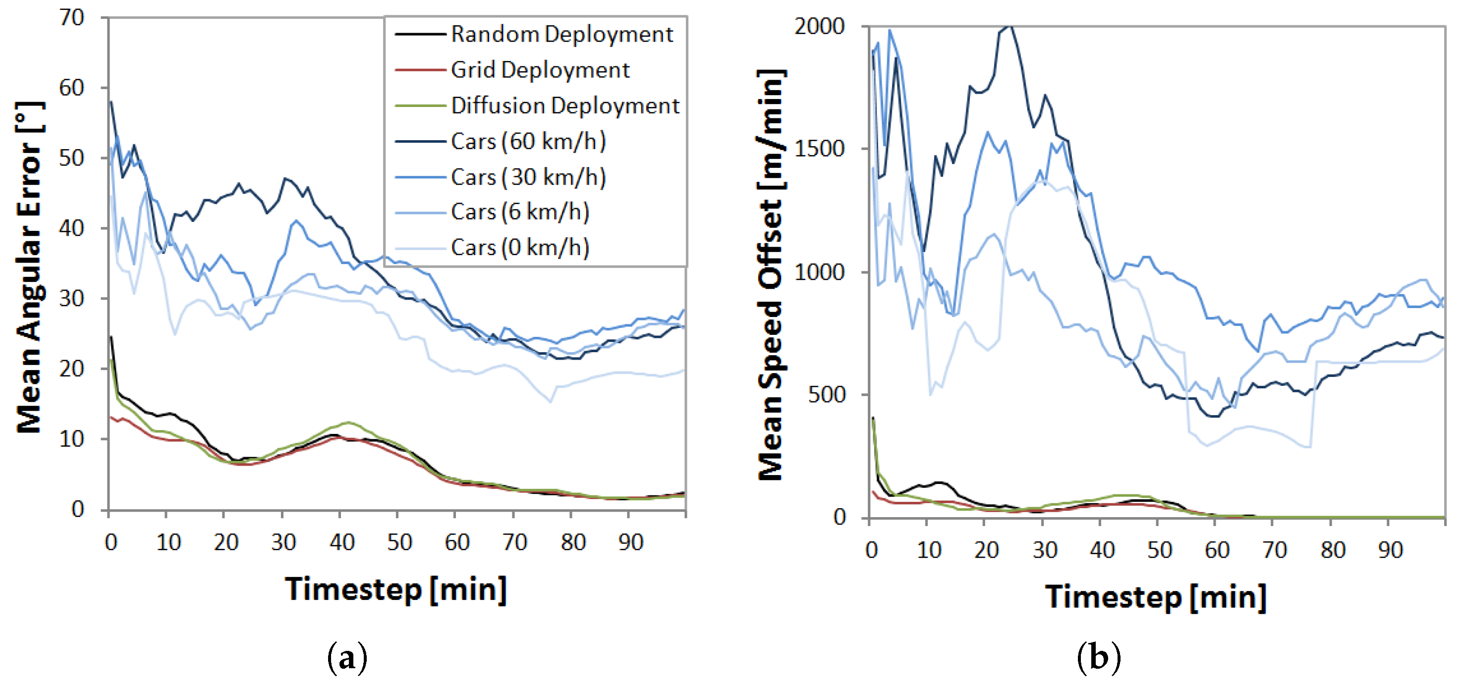
• Deployment and stationarity of nodes: When the number of nodes and communication distance are held fixed, the deployment strategy of stationary nodes does not have a large influence on the motion estimation results (Figure 6). However, with decreasing node density, the performance of a random deployment will certainly decrease, since there will be disconnected nodes. Further, the algorithm has been developed for stationary nodes. Nonetheless, it can also be applied in a non-stationary setting, e.g., for cars. However, then the motion estimation accuracy decreases (Figure 6) due to the increased error in the temporal derivative estimate and the linear alignment of the cars along roads.

Future work includes the analysis of the motion state error of the Kalman filter, which is an important measure in practice. In addition, error-in-variables models could be investigated for replacing the Kalman filter for motion estimation, e.g., a total least squares method accounting for errors in the estimates of spatial derivatives directly. Further, simulations for longer time periods, such as days or weeks, are necessary in order to evaluate the behavior of the algorithm under changing motion conditions. The simulations of VANETs have shown that in order to achieve satisfying and reliable results in a non-stationary setting, more work is required on the algorithm. For example, integrating the estimation of the temporal derivative into the least squares adjustment for estimating the partial derivatives or including an error term for the temporal derivative estimate. Finally, the ultimate goal is to replace the simulated network with a real deployment of a GSN and real measurements of a moving atmospheric or oceanographic field.

References

1. Govindaraju, R.S. Artificial neural networks in hydrology. I: Preliminary concepts. J. Hydrol. Eng. 2000, 5, 115–123. [Google Scholar]
2. Taormina, R.; Chau, K.W. Data-driven input variable selection for rainfall-runoff modeling using binary-coded particle swarm optimization and Extreme Learning Machines. J. Hydrol. 2015, 529 Pt 3, 1617–1632. [Google Scholar] [CrossRef]
3. Farnebäck, G. Two-Frame motion estimation based on polynomial expansion. In Image Analysis; Number 2749 in Lecture Notes in Computer Science; Bigun, J., Gustavsson, T., Eds.; Springer: Berlin/Heidelberg, Germany, 2003; pp. 363–370. [Google Scholar]
4. Lin, C.; Vasić, S.; Kilambi, A.; Turner, B.; Zawadzki, I. Precipitation forecast skill of numerical weather prediction models and radar nowcasts. Geophys. Res. Lett. 2005, 32, L14801. [Google Scholar] [CrossRef]
5. Bowler, N.E.; Pierce, C.E.; Seed, A. Development of a precipitation nowcasting algorithm based upon optical flow techniques. J. Hydrol. 2004, 288, 74–91. [Google Scholar] [CrossRef]
6. Fitzner, D.; Sester, M. Estimation of precipitation fields from 1-minute rain gauge time series–comparison of spatial and spatio-temporal interpolation methods. Int. J. Geogr. Inf. Sci. 2015, 29, 1668–1693. [Google Scholar] [CrossRef]
7. Cohen, I.; Herlin, I. Optical flow and phase portrait methods for environmental satellite image sequences. In Computer Vision—ECCV ’96; Number 1065 in Lecture Notes in Computer Science; Buxton, B., Cipolla, R., Eds.; Springer: Berlin/Heidelberg, Germany, 1996; pp. 141–150. [Google Scholar]
8. Haberlandt, U.; Sester, M. Areal rainfall estimation using moving cars as rain gauges—A modelling study. Hydrol. Earth Syst. Sci. 2010, 14, 1139–1151. [Google Scholar] [CrossRef] [Green Version]
9. Fitzner, D.; Sester, M.; Haberlandt, U.; Rabiei, E. Rainfall estimation with a geosensor network of cars theoretical considerations and first results. Photogramm. Fernerkund. Geoinform. 2013, 2013, 93–103. [Google Scholar] [CrossRef]
10. Black, M.J. Robust Incremental Optical Flow. Ph.D. Thesis, Yale University, New Haven, CT, USA, 1992. [Google Scholar]
11. Duckham, M. Decentralized Spatial Computing: Foundations of Geosensor Networks; Springer: Berlin/Heidelberg, Germany, 2012. [Google Scholar]
12. Lucas, B.D.; Kanade, T. An iterative image registration technique with an application to stereo vision. In Proceedings of the 7th International Joint Conference on Artificial Intelligence (IJCAI), Vancouver, BC, Canada, 24–28 August 1981.
13. Kalman, R. A new approach to linear filtering and prediction problems. J. Basic Eng. 1960, 82, 35–45. [Google Scholar] [CrossRef]
14. Fitzner, D.; Sester, M. Decentralized gradient-based field motion estimation with a wireless sensor network. In Proceedings of the 5th International Confererence on Sensor Networks, Rome, Italy, 19–21 February 2016; pp. 13–24.
15. Barron, J.L.; Fleet, D.J.; Beauchemin, S.S. Performance of optical flow techniques. Int. J. Comput. Vis. 1994, 12, 43–77. [Google Scholar] [CrossRef]
16. Sester, M. Cooperative boundary detection in a geosensor network usng a SOM. In Proceedings of the International Csrtographic Conference, Santiago, Chile, 15–21 November 2009.
17. Jeong, M.H.; Duckham, M.; Kealy, A.; Miller, H.J.; Peisker, A. Decentralized and coordinate-free computation of critical points and surface networks in a discretized scalar field. Int. J. Geogr. Inf. Sci. 2014, 28, 1–21. [Google Scholar] [CrossRef]
18. Umer, M.; Kulik, L.; Tanin, E. Spatial interpolation in wireless sensor networks: Localized algorithms for variogram modeling and Kriging. GeoInformatica 2010, 14, 101–134. [Google Scholar] [CrossRef]
19. Brink, J.; Pebesma, E. Plume tracking with a mobile sensor based on incomplete and imprecise information. Trans. GIS 2014, 18, 740–766. [Google Scholar] [CrossRef]
20. Das, J.; Py, F.; Maughan, T.; O’Reilly, T.; Messié, M.; Ryan, J.; Sukhatme, G.S.; Rajan, K. Coordinated sampling of dynamic oceanographic features with underwater vehicles and drifters. Int. J. Robot. Res. 2012, 31, 626–646. [Google Scholar] [CrossRef]
21. Tsai, H.W.; Chu, C.P.; Chen, T.S. Mobile object tracking in wireless sensor networks. Comput. Commun. 2007, 30, 1811–1825. [Google Scholar] [CrossRef]
22. Horn, B.K.; Schunck, B.G. Determining optical flow. Artif. Intell. 1981, 17, 185–203. [Google Scholar] [CrossRef]
23. Langley, R.B. Dilution of precision. GPS World 1999, 10, 52–59. [Google Scholar]
24. Niemeier, W. Ausgleichungsrechnung: Eine Einführung für Studierende und Praktiker des Vermessungs- und Geoinformationswesens; de Gruyter: Berlin, Germany; New York, NY, USA, 2002. [Google Scholar]
25. Simoncelli, E.P. Distributed Representation and Analysis of Visual Motion. Ph.D. Thesis, Massachusetts Institute of Technology, Department of Electrical Engineering and Computer Science, Cambridge, MA, USA, 1993. [Google Scholar]
26. Simoncelli, E.P.; Adelson, E.H.; Heeger, D.J. Probability distributions of optical flow. In Proceedings of the 1991 IEEE Computer Society Conference on Computer Vision and Pattern Recognition, Los Alamos, CA, USA, 3–6 June 1991.
27. Särkkä, S. Bayesian Filtering and Smoothing; Cambridge University Press: Cambridge, UK, 2013. [Google Scholar]
28. Watson, P.K. Kalman filtering as an alternative to Ordinary Least Squares—Some theoretical considerations and empirical results. Empir. Econ. 1983, 8, 71–85. [Google Scholar] [CrossRef]
29. Berndt, C.; Rabiei, E.; Haberlandt, U. Geostatistical merging of rain gauge and radar data for high temporal resolutions and various station density scenarios. J. Hydrol. 2014, 508, 88–101. [Google Scholar] [CrossRef]
30. Schulz, F. Modeling sensor and ad hoc networks. In Algorithms for Sensor and Ad Hoc Networks; Springer: Heidelberg, Germany, 2007; pp. 21–36. [Google Scholar]
31. Golub, G.H.; Loan, C.F.V. Matrix Computations; JHU Press: Baltimore, ML, USA, 1996. [Google Scholar]
Figure 1. Time series of weather radar images (original size 230 × 230 pixels with a pixel resolution of 1 km 2 ) separated by 20 min from left to right. Motion vectors estimated with an optical flow algorithm.
Ijgi 05 00175 g001
Figure 2. The 10 km × 10 km study area for the motion estimation algorithms. OSM, Open Street Map.
Ijgi 05 00175 g002
Figure 3. Deployment strategies. (a) Completely random deployment; (b) grid deployment; (c) diffusion deployment around a central node; (d) vehicular ad hoc network (VANET).
Ijgi 05 00175 g003
Figure 4. Homogenous field (a); and more heterogeneous, non-linear field (b). Randomly-distributed set of nodes with simulated spatio-temporal field and estimated (c) and true (d) field motion per time step. Red indicates high, blue zero field values.
Ijgi 05 00175 g004
Figure 5. Comparison of the angular error and speed offset for different motion speeds and the two field types. (a) Mean angular error per time step for n = 400 and r = 500 m; (b) mean speed offset per time step for n = 400 and r = 500 m; (c) mean angular error per time step for n = 25 and r = 2000 m; (d) mean speed offset per time step for n = 25 and r = 2000 m.
Ijgi 05 00175 g005
Figure 6. Comparison of the angular error and speed offset for different geosensor network (GSN) deployments. (a) Mean angular error per time step; (b) mean speed offset per time step.
Ijgi 05 00175 g006
Figure 7. Comparison of the angular and speed offset for different Kalman filer measurement noise parameters. (a) Mean angular error; (b) mean speed offset; (c) standard deviation angular error; (d) standard deviation speed offset.
Ijgi 05 00175 g007
Figure 8. Characterization of the radar event. (a) Time series of radar estimated rainfall averaged over the study area; (b) time series of mean motion direction calculated by image-based optical flow; (c) time series of the mean motion speed calculated by optical flow. Time steps of no data values result from the inability of the optical flow (OF) algorithm to detect field motion when there is no rainfall.
Ijgi 05 00175 g008
Figure 9. Time series of radar images separated by 1 min from the upper left to the lower right for the first rain cloud in the event (Time Steps 14 to 23). Simulated sensor network of n = 25 nodes, a communication range of r = 2000 m and estimated motion vectors.
Ijgi 05 00175 g009
Figure 10. Results of the motion estimation algorithm for the two different node densities. (a) Time series mean angular error; (b) time series of estimated motion direction averaged over all nodes; (c) time series of estimated motion speed averaged over all nodes.
Ijgi 05 00175 g010