Forecasting Public Transit Use by Crowdsensing and Semantic Trajectory Mining: Case Studies

Abstract

With the growing development of smart cities, public transit forecasting has begun to attract significant attention. In this paper, we propose an approach for forecasting passenger boarding choices and public transit passenger flow. Our prediction model is based on mining common user behaviors for semantic trajectories and enriching features using knowledge from geographic and weather data. All the experimental data comes from the Ridge Nantong Limited bus company and Alibaba platform which is also open to the public. We evaluate our approach using various data sources, including point of interest (POI), weather condition, and public bus information in Guangzhou to demonstrate its effectiveness. Experimental results show that our proposal performs better than baselines in the prediction of passenger boarding choices and public transit passenger flow.

1. Introduction

In recent years, geosensor networks and the sensor web have rapidly expanded in smart cities. Geosensors, such as card and bus GPS terminals, produce massive datastreams every day. These data from crowdsensing [1] are of high value in some fields and can be mined to produce useful knowledge for decision-making purposes. As a city expands and its population increases, the city’s public transit system bears significant pressure. For example, commuters usually have to deal with crowded buses or subways in order to get to work, which is inconvenient and unpleasant. Additionally, it can be difficult for both private sector and government transit providers to arrange reasonable routes and predict the potential future flow of passengers. Therefore, the ability to forecast public transit needs is beneficial.

Luckily, government departments are increasingly willing to provide open access to city data (e.g., through data.org ), which is useful for researchers who aim to tackle real-world problems. The provincial government of Guangdong and the Ridge Nantong Limited bus company held a competition to predict passenger boarding choices and flow on the Alibaba platform [2], which provides millions of user behavior datastreams along several public transport routes. Predicting passengers’ boarding choices is a user behavior analysis that may provide residents with a more intelligent public transport service and better timing of directional advertising. Moreover, passenger flow prediction in public transit is helpful for traffic control decision-making by the transit provider and government.

Issues related to mining frequent patterns in mobile users’ trajectories that have been discussed in the existing studies mostly consider the geographic features of trajectories [3,4]. However, patterns based on geographic trajectories are constrained by geographic data and do not work well when considering unvisited locations. Conversely, semantic trajectories have been proposed by Bogorny et al. [5]. Practically, a semantic trajectory consists of a list of locations labeled with semantic tags that may indicate the activities being carried out in these trajectories. For instance, we may mine user trajectories with semantic tags like <Community, Education, Community>, which reveal the semantic behaviors of the user. However, different people have different travel requirements. For example, there is a rigid demand for office workers to go to work in the morning and back home at night (i.e., during rush hours); while for the elderly, travel times are usually more uncertain. Moreover, different weather conditions and district or neighborhood functions have different impacts on traveling. For example, office workers must go to work and back home on weekdays, no matter how bad the weather is; however, when the weather is bad during the weekend, they will not go out. In contrast, the elderly may go out on nice days whether it is a weekend or a weekday. Additionally, a district’s function may constrain passengers’ actions. For instance, office workers normally get off the bus near a city’s central business district in the morning, while the elderly usually arrive at a station near a park or supermarket.

In this paper, we propose a method for forecasting public transit in the coming week. We first preprocess the raw data (using a schema illustrated in the Appendix), filtering out dirty data and discretizing what remains. Then, we annotate the data with semantic information. We construct several feature vectors and train the data with XGBoost [6]. We present two case studies: (1) Forecasting the boarding choices of passengers, predicting whether a passenger will or will not take the bus; (2) Forecasting public transit passenger flow, predicting how many passengers will take the bus.

The major contributions of this paper are as follows:

(1)

We present a approach for forecasting public transit using crowdsensing.

(2)

We present two case studies of forecasting public transit boarding choices and passenger flow.

(3)

We evaluate our approach using various data sources, including point of interest (POI), weather condition, and public bus information in Guangzhou to demonstrate its effectiveness.

The remainder of this paper is organized as follows. Section 1 briefly reviews existing studies on trajectory prediction. Section 2 contains the framework, data preprocessing, semantic trajectories mining, and feature information. In Section 3, we present the results of our experiments. Finally, Section 4 summarizes our findings and concludes the paper with a brief discussion of the scope of our future work.

2. Related Work

2.1. User Behavior Mining

There are two main approaches for understanding user behavior mining, known as frequent pattern and random walk. Firstly, Jiang et al. [7] studied taxi trajectories and found that they follow Levy flight (A random walk in which the steps are defined in terms of the step-lengths, which have a certain probability distribution, with the directions of the steps being isotropic and random.) behavior. Titus et al. [8] investigated the Brownian motion and Brownian bridges with arbitrary endpoints. However, Song et al. [9] found that only $93\%$ of users’ short-term mobility can be predicted, meaning that random walk-based methods do not work well for long-term predictions. Additionally, there are kinds of frequent patterns utilized, such as spatial-temporal sequential [10], semantic-geographic [11], and mobile sequential patterns [12]. In fact, many user behaviors have semantic meanings. Alvares et al. [11] proposed to explore geographic and semantic properties by mining semantic trajectory patterns from mobile users’ location histories. Ying et al. [13] proposed a mining-based location prediction approach called geographic-temporal-semantic-based location prediction (GTS-LP), which takes into account a user’s geographic-triggered intentions. However, there exist many other factors that affect users’ movements, such as weather, time, and holidays.

2.2. Prediction Model Building

Existing studies that make predictions about user behaviors can be classified into three categories: those that utilize individual user data; those that utilize crowd-generated data; and hybrid methods using all data. The prediction model in [14] is based on an eigenvector space modeling regular user movement in order to predict a user’s next location. Such a prediction model does not consider historical user movement, which results in poor performance. Normally, using only a user’s individual data does not work well. In contrast, the prediction model in [15] is based on a social-spatial approximation that utilizes the current GPS coordinates of a user’s friends to estimate the GPS coordinate of the user. However, these methods do not consider the user’s current movements. For example, even though the user frequently visits a gym, the probability of him visiting the gym after visiting the swimming pool must be very low. Monreale et al. [16] proposed a hybrid method that not only considers a user’s own data but also utilizes data generated by crowds. However, these models focus only on user movements motivated by semantic and geographic-triggered intentions, whereas different weather conditions or area functions (Education/Business) may alter users’ final destinations.

There exist many forecasting methods. The artificial neural network is obviously a convenient model for prediction. However, the training and optimization of parameters of neural networks is time consuming. XGBoost [6] is a large-scale machine learning method that can be used to build scalable learning systems. XGBoost has been used by a series of applications solutions, which performs well in real situations. This proves the efficacy of this method, which is fast and optimized for out-of-core computations. Methods using boosted trees have been in use for some time. They are trained with decision trees of fixed size as a base learner, which is robust to outliers. As a tree-based algorithm, gradient-boosting decision trees (GBDTs) can also handle non-linear feature interactions.

3. Approach

3.1. Framework

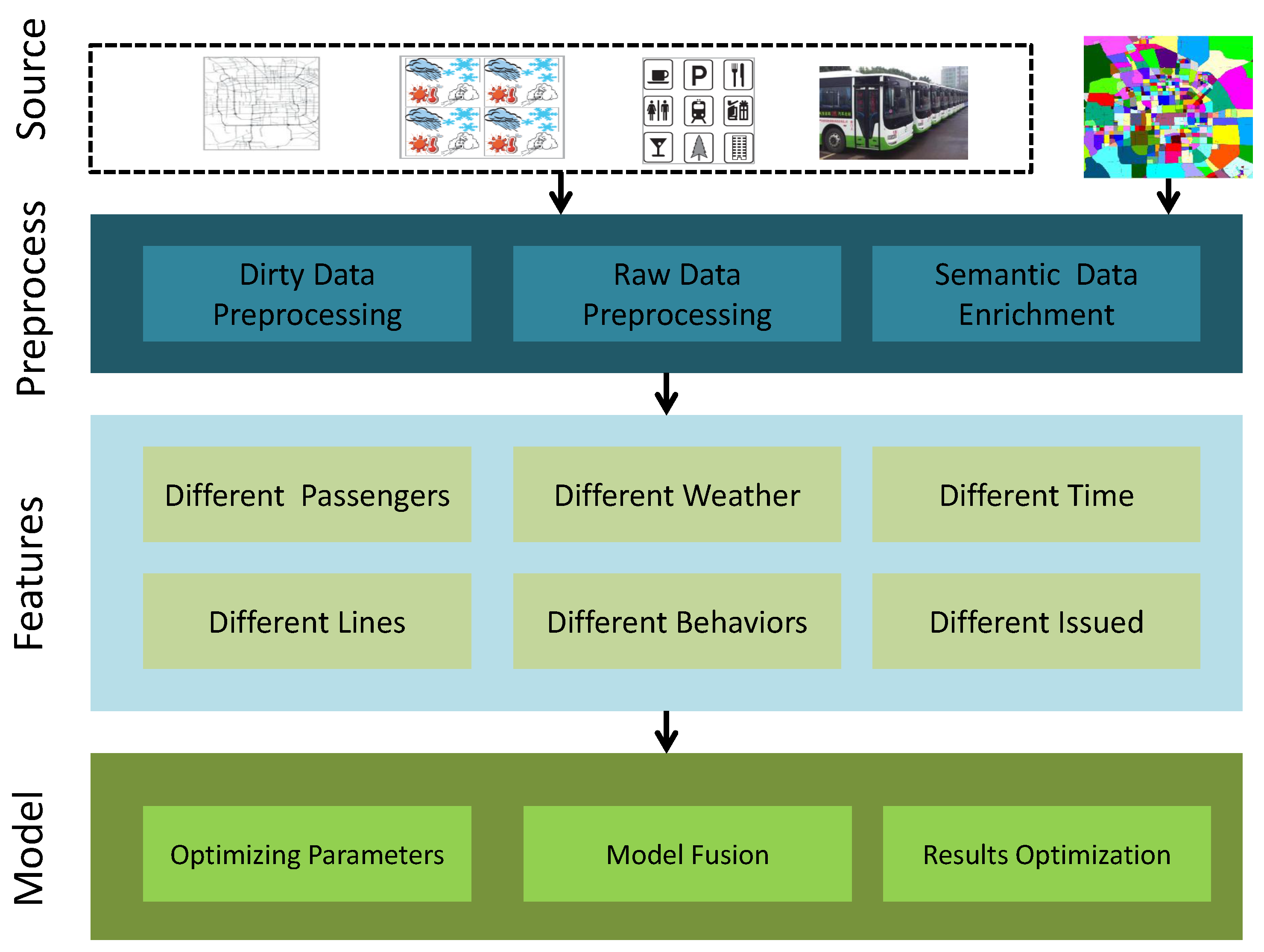
As Figure 1 shows, our framework consists of two parts: feature engineering and model building. We first preprocess the raw data to filter out dirty data and discretize the dataset. Then, we annotate the data with semantic information. We construct several feature vectors and train with these data.

Problem statement: Given bus card record datasets over a period of several months (1 August 2014–31 December 2014), each of which includes the bus card ID, terminal ID (bus stop ID), travel time, etc., our problem is (1) a binary classification and (2) a regression task. We aim to predict, for the following week (1 January 2015–7 January 2015) (1) whether a specific passenger will take a specific bus, by predicting the existence label $y\in \{0,1\}$ in these records ($Card\_id,Line\_name$), and (2) the passenger numbers for a bus line, as ($Line\_name,Deal\_date,Deal\_hour,\mathbf{Passenger}\_\mathbf{count}\mathbf{\left(}\mathbf{prediction}\mathbf{\right)}$).

3.2. Data Preprocessing

3.2.1. Dirty Data Preprocessing

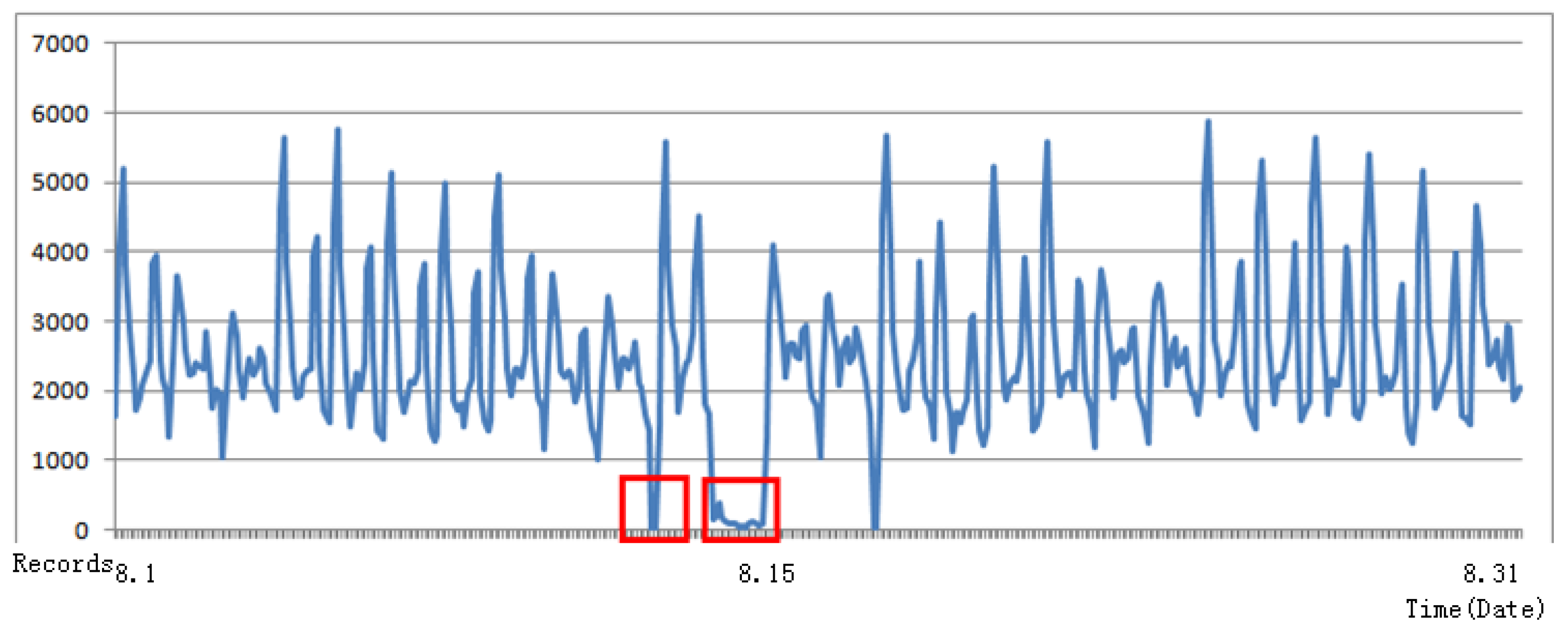
Figure 2 shows the different kinds of dirty data that exist in practice. The horizontal coordinate is time and the vertical coordinate is the total number of records of Bus Line 1. Entering this raw data into the training model will not produce a reasonable result, so it is of key importance to preprocess the data. About $40\%$ of the raw data have a $terminal\_id$ that corresponds with more than two $line\_name$ values. We divide the $terminal\_id$ into two categories: $terminal\_id$ with one $line\_name$ and those with two or more values of $line\_name$. This procedure has practical significance, because it filters out the passengers with regular bus lines. All the features are generated separately. Moreover, there exist some data for which the same $card\_id$ has more than two records in the same $line\_name$ at the same time. This is very abnormal and may be caused by terminal equipment or data transmission failures. We rank these $card\_id$ records in the same $line\_name$ at the same time and filter out all duplicate records.

3.2.2. Raw Data Preprocessing

In addition to dirty data, many kinds of data cannot be used directly for training, such as weather condition, time, and so on. We have to consider records with the same conditions (e.g., weather, time, etc.) of records $Card\_id$ and $Line\_name$ and construct the features. Take weather as an example: we have to calculate the number of records of the same weather condition in the last few hours, days, and so on, which can measure the difference of passengers in different weather conditions. In many machine learning tasks, the feature is not always a continuous value, but it is likely to be the value of the classification. For example, the temperature classes can describe the temperature in certain weather conditions while the continuous variables cannot. We make these data discrete by adopting dummy variables to handle them data. For instance, the daytime temperature is recorded as "0001" for the condition in which $temperatur{e}_{day}\ge$ 10 ${}^{\circ }$C and $temperatur{e}_{day}\le$ 20 ${}^{\circ }$C , which is widely used in category features and has two advantages: (1) solve the problem of the classifier is not good to deal with attribute data and, (2) to a certain extent, it expands the characteristic of features. We thus transform the weather condition and time data. The daytime temperature is divided into (10 ${}^{\circ }$C–20 ${}^{\circ }$C), (20 ${}^{\circ }$C–30 ${}^{\circ }$C), and (>30 ${}^{\circ }$C) and the nighttime temperature is divided into (0 ${}^{\circ }$C–10 ${}^{\circ }$C), (10 ${}^{\circ }$C–20 ${}^{\circ }$C), and (20 ${}^{\circ }$C–30 ${}^{\circ }$C). The time data are divided into weekday, weekend, holiday, and rush hour.

3.3. Semantic Trajectory Mining

We divide a city into disjointed blocks [17], assuming that placement in a block g is uniform. The road network is usually composed of a number of major roads, such as the ring road, and the city is divided into areas [18]. We map the projection of the vector-based road network onto a plane and convert it to a raster model [19]. Each pixel of the image of the projected map can be viewed as a block element of the corresponding raster map. Consequently, the road network is converted into a binary image. Then, we extract the skeleton of the road, while retaining the original two-value image topology. Finally, we obtain the blocks g of the cities.

Each bus stop has latent semantic meaning due to its surroundings, such as POIs and neighborhood function. For example, a passenger who gets on the bus at a station in a residential area and gets off near a school every day may be going to school at a fixed time. We can formulate these records as <Community, Education>. The "Community" refers to the region of residential quarters with many people living there. We follow the approach of Ying et al. [13] to mine semantic patterns from each user’s records. Semantic location information is labeled from the Baidu Map API (data schema shown in the Appendix). We use some general categories, such as POI type and neighborhood function, as semantic labels. If a record location overlaps one or several areas with semantic labels, the semantic meanings of these areas are assigned to this record. 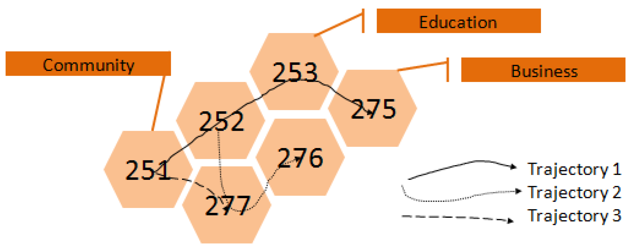Figure 3 shows that the semantic label of block 253 (Block ID) is Education. We transform each passenger record to a semantic record, like <$Community,Education$>. Primary user behaviors may exhibit some patterns, and thus can be predicted. Formally, there are n categories (including both POIs and neighborhood function) of blocks $\{l_1,l_2,...,l_n\}$, where $l_i$ is a category such as Education (function) or Coffee Shop (POI). The bus records of passengers are represented in such combinations (231 combinations in this paper) $\{(l_1,l_2),(l_1,l_3),...,l_i,l_j,...,(l_{n-1},l_n)\}$. Each combination represents a different user travel behavior.

3.4. Forecasting Passenger Boarding Choice

For this task, we consider the combinations of features $Card\_id$ and $Line\_name$, and the association of a particular bus card with this bus line. Our features consist of seven categories: (1) Passenger (2) Bus Line (3) Time (4) Weather (5) Bus Card Issuing Location (6) Bus Card and (7) Latent Semantic User Behavior features. Specifically, we calculate these features for each day. We calculate the total number of records; the number of hours, days, and weeks that have records; and the number of times the card appears at different terminals (bus stops) over the past 1, 3, 7, 28, 70 and 126 days for the combination of $Card\_id$ and $Line\_name$. The specific days are chosen because the data have periodicity over a week. Take the weather feature as an example. We consider records with the same weather condition of records $Card\_id$ and $Line\_name$ and calculate the features. Formally, we have:

• $F=\{F_{passenger},F_{bus},F_{time},F_{weather},F_{issued},F_{card},F_{semantic}\}$
• $F_i=\{f_{1day},f_{3day},f_{7day},f_{28day},f_{70day},f_{125day}\}$
• $f_i=\{Total\_Records,Hours,Days,Weeks,Times\_Different\_Terminals\}$

where $F_i$ is calculated considering the feature type. For instance, if i is $time$ (we divide time into in four categories, described in Section 3.2.2), we consider records with the same time condition (e.g., rush hour, weekday) as $Card\_id$ and $Line\_name$.

3.5. Passenger Flow Forecasting

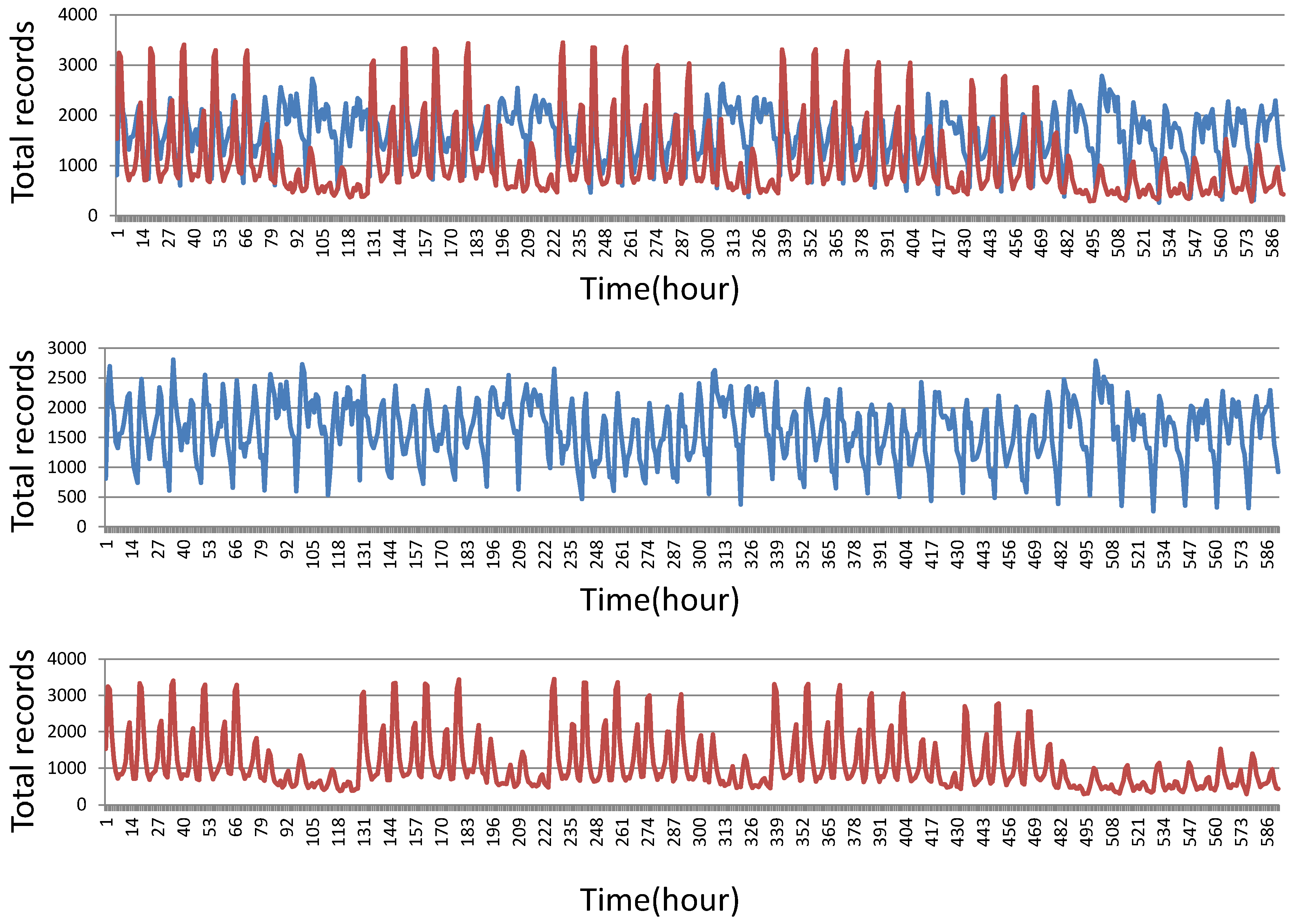
Three methods for passenger flow forecasting exist: (1) directly gathering all passenger boarding choice forecasting data to get the total number of bus passengers; (2) making the daily regression prediction using total passenger numbers; and (3) user group classification and data gathering. We adopt the third approach because of the great individual differences in bus records. The simple superposition of user records cannot be a good reflection of overall data trends because there are two kinds of passengers, as shown in Figure 4. The red line shows occasional passengers and the blue line shows frequent passengers from 1 September 2014 to 7 October 2014. The records of frequent passengers are regular while the records of occasional passengers are random. We build different models for these different kinds of passengers. The $Y_{rand}$ is the prediction result of random passenger model while the $Y_{freq}$ is the prediction result of frequent passenger model. We have to combine the two results and get the final result. However, on different days (weekend/holiday and weekday), the portion of random passengers or frequent passengers in the total passengers are different. We use the variable α and β to adjust this deviation. Formally, we have:

$$Y=\left\{\begin{array}{ccccc}\alpha \ast Y_{freq}+Y_{rand}\hfill & & ifY\hfill & & \in weekendandholiday\hfill \\ \beta \ast Y_{freq}+Y_{rand}\hfill & & ifY\hfill & & \in weekday\hfill \end{array}\right.$$

We calculate the total number of passengers in each hour of each line and adopt one-hot encoding of weather conditions and semantic user behaviors as features for regression.

4. Experiments

4.1. Setup

All of our experimental data are available online. The dates of the public transit data range from 1 August 2014 to 31 December 2014. We use the data from 1 December 2014 to 31 December 2014 as the training data and from 1 January 2015 to 7 January 2015 as test data. The data ranged from 06:00 to 20:00 each day and data schema description details are in the Appendix. We obtain POI and district function data from the Baidu Map API [20]. We obtain free-text place descriptions using geoparsing [21] to convert text into unambiguous geographic identifiers (latitude and longitude coordinates). We train our data with XGBoost [22], optimizing its parameters by a linear weighted method. We set $\alpha =1.21$ and $\beta =0.95$. We mainly tune the parameters, including the maximum depth of tree and the step size shrinkage used in updates, to prevent overfitting and to minimize the sum of the instance (Hessian) weight needed in a child node. Finally, we set the maximum depth to 10, step size to 0.3, and the minimum instance weight sum to 2.0 in our experiments. Logistic regression [23] and linear regression are used as weak classifier in our experiment.

4.2. Metrics

First, we use the set of baselines to justify the necessity of each component of our method by, for example, not utilizing user behavior ($F_{semantic}$) or the weather ($F_{weather}$).

To forecast passenger boarding choice, we adopt logistic regression [23], GBDTs [24], and Random Forests [25] as baselines. For passenger flow forecasting, we use Autoregressive-moving Average (ARMA) [26], a single layer artificial neural network (ANN), and linear regression as baselines.

Specifically, we have:

$$Precision=\frac{|\bigcap (PredictionSet,ReferenceSet\left)\right|}{\left|PredictionSet\right|}$$

(1)

$$Recall=\frac{|\bigcap (PredictionSet,ReferenceSet\left)\right|}{\left|ReferenceSet\right|}$$

(2)

We evaluate the final result with F1 scores, where $F1=\frac{2\times Precision\times Recall}{Precision+Recall}$, for the passenger boarding choice forecasting.

For passenger flow forecasting, we adopt the root mean square error (RMSE), defined as $RMSE=\sqrt{\frac{{\sum }_i^n{(y_i-{\widehat{y}}_i)}^2}{n}}$, where ${\widehat{y}}_i$ is a prediction and $y_i$ is the ground truth.

4.3. Data Insight

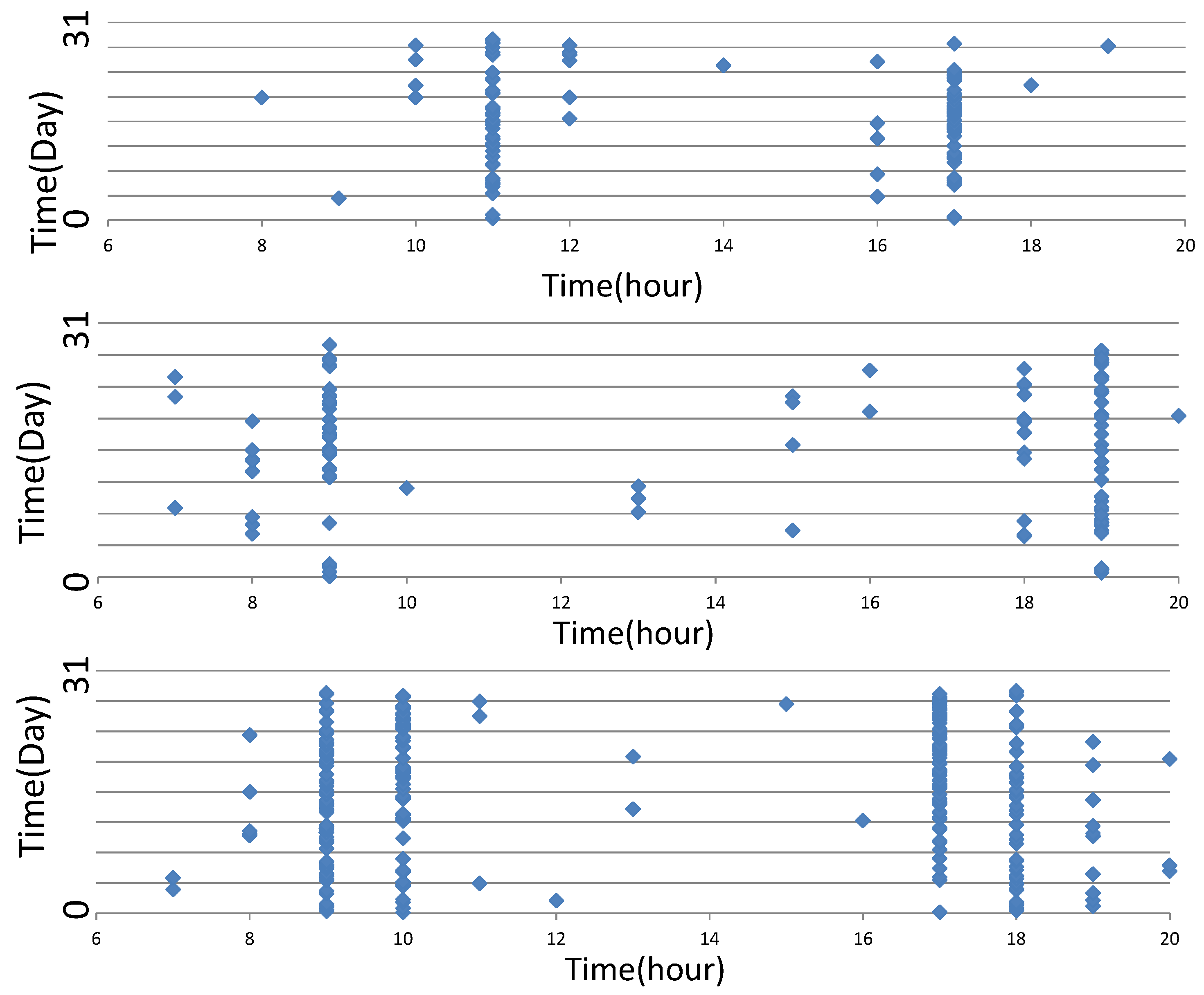
We first analyze individual public transit records. As Figure 5 depicts, the horizontal coordinates represent the hour (06:00–20:00) of travel and the vertical coordinates represent the travel date (the 1st–31st day of the month). There exist significant differences between individuals. Take Line 1 as an example: there are 19,513,511 passengers and 6,738,391 records over five months, meaning that there are 3.45 passengers per record over this period. This result indicates that there are many passengers who rarely take the bus. We then divide those passengers by their travel record frequency. Passengers with more than eight records each week are treated as frequent passengers, while the others are occasional passengers. 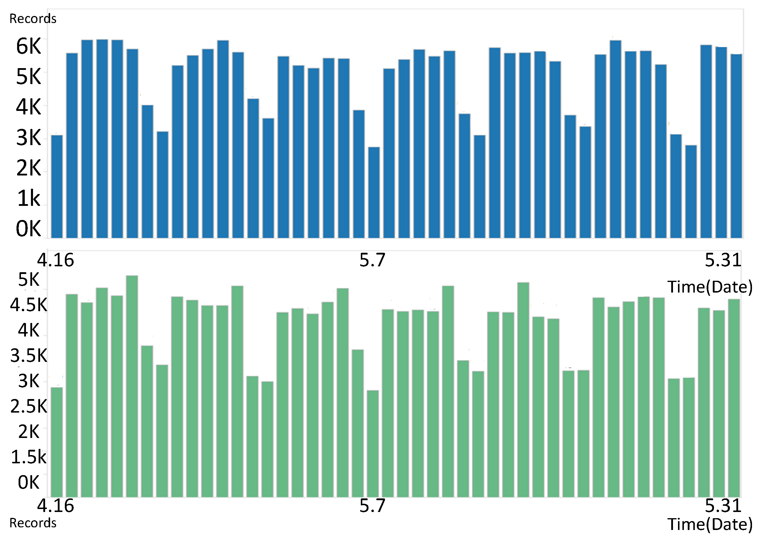As Figure 6 shows, the blue histogram represents the flow of frequent passengers and the green, occasional passengers. Clearly, the two groups follow different rules regarding travel times. Hence, we build different passenger flow forecasting models for frequent and occasional passengers.

4.4. Results

4.4.1. Forecasting Passenger Boarding Choices

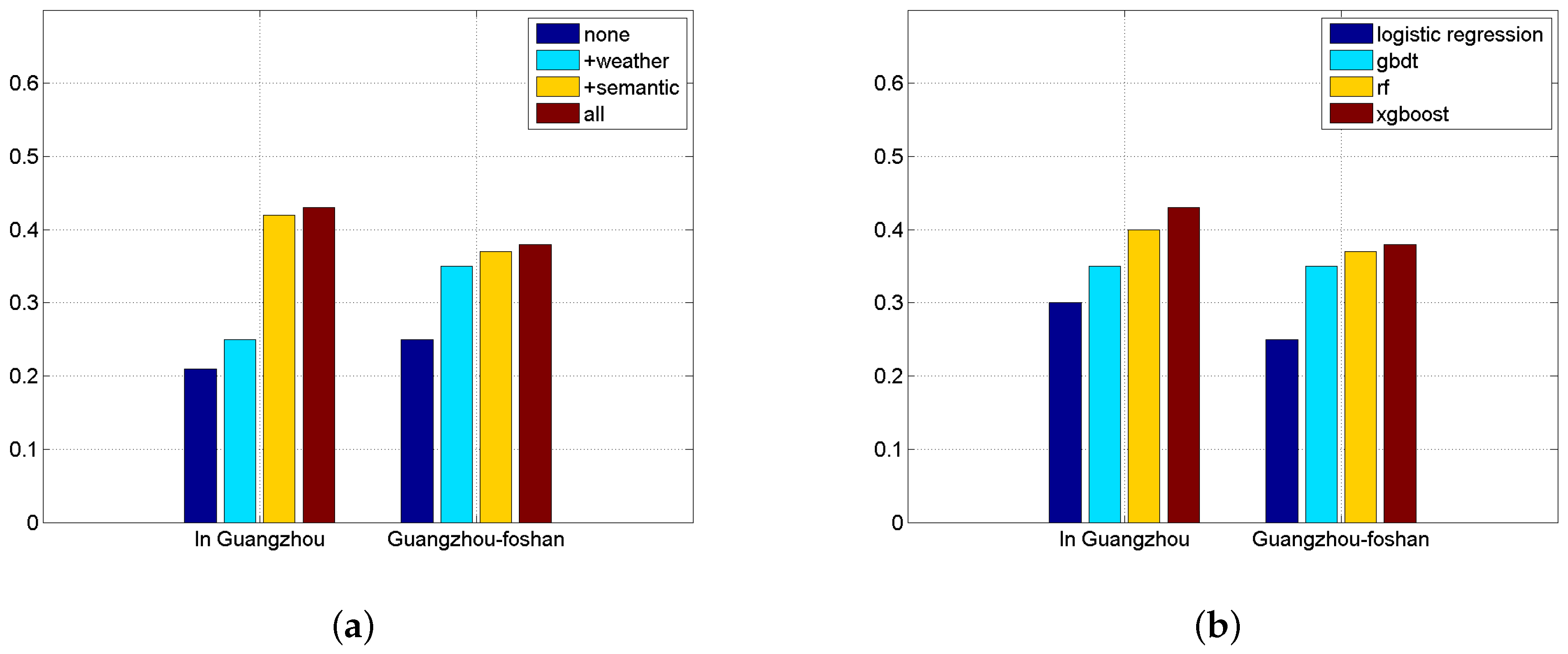
Figure 7a demonstrates the necessity of each component of our method for forecasting passenger boarding choices. The “none” case adopts only time features and has the worst results. By adding weather and semantic features, F1 scores increase rapidly. The “all” case utilizes all the features of our method and gets the best results. Figure 7b shows the results of logistic regression, GBDT, Random Forest, and XGBoost. XGBoost shows good performance compared with the other methods.

4.4.2. Passenger Flow Forecasting

Figure 8a shows the necessity of each component of our method for passenger flow forecasting. The “none” case adopts only time features and has the worst results. By adding weather and semantic features, F1 scores increase rapidly. The “all” case adopts all the possible features of our method and gets the best results. Figure 8b shows the results of linear regression, ANN, ARMA, and XGBoost. XGBoost has superior performance compared to the other methods.

4.5. Case Studies: Public Transport in Guangzhou

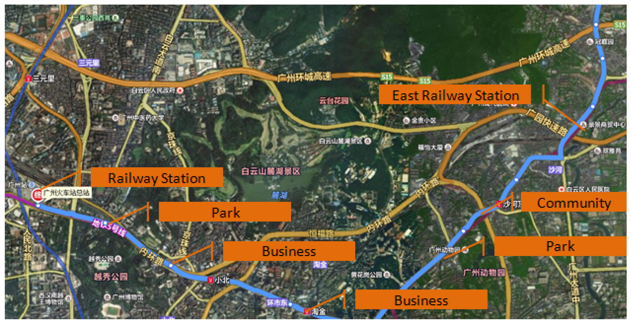
Bus data is not just traffic data. It can reveal users’ potential travel needs. As Figure 9 shows, passengers who get on a bus at the Railway Station and get off at the East Railway Station may want to change trains. The passengers from a Shahe (Community) to Xiaobei (Business) may be going to work, while those who travel from Shahe (Community) to the Zoo (Park) may be traveling for entertainment purposes. The frequency and timing of public transit trips can also indicate potential reasons for traveling and reflect the pulse of a city.

4.6. Discussion

Good solutions are derived from a thorough understanding of business and detailed data analysis. Today, the significance of mobile applications such as Uber and Didi (an Uber-like app in China) lies in connecting people and travel tools. However, this shared economic model is far from economic. Imagine that when Uber and Didi were launched, the frequency of car travel increased significantly, leading to a decline in the frequency of public transit use and a consequent increase in traffic congestion and environmental pollution. Public transit is much more economic and environmentally friendly than private car travel and there still exist severe traffic congestion and environmental problems in big cities. Hence, the development of public transit is more urgent than that of private cars, even though travellers may find public transit less convenient and comfortable. Based on the analysis of big datasets, such as public transport and road network data from smart cities, we can improve the convenience, comfort, ease, and speed of travel via public transit. Moreover, directional advertising timing can be provided by passenger behavior analysis. In recent years, more data have become accessible through web services in order to mine their potential value. Analyzing these data can improve social efficiency.

5. Conclusions

In this study, we propose an approach for forecasting public transit using crowdsensing data, which is helpful for public transit companies and government decision-making, but had not previously been investigated. In this framework, we first preprocess the raw data to filter out dirty data to discretize the dataset. Next, we annotate the data with semantic information, construct several feature vectors, and train with those data.

There are some limitations to this study, which should be addressed in future work. One major limitation lies in the partially missing data from some users and the limited availability of open data. For example, there exist many records that do not record when the passenger got off the bus (passengers should use their bus card both to get on and off the bus/subway). We would like to mine the passenger behaviors more deeply in the future. The adaptability of this approach to real-world circumstances will also be considered in our future work. First, some visual analytics functions will be added to our ongoing demonstration system. Through presenting similar historical circumstances or forecasting results according to different features, the system will be able to provide more information for flexible decision-making. We are also investigating a new prediction model that utilizes data from similar historical circumstances through understanding the underlying semantics of the data.