Figure 1.
Plan view for RNP segment width.
Figure 1.
Plan view for RNP segment width.
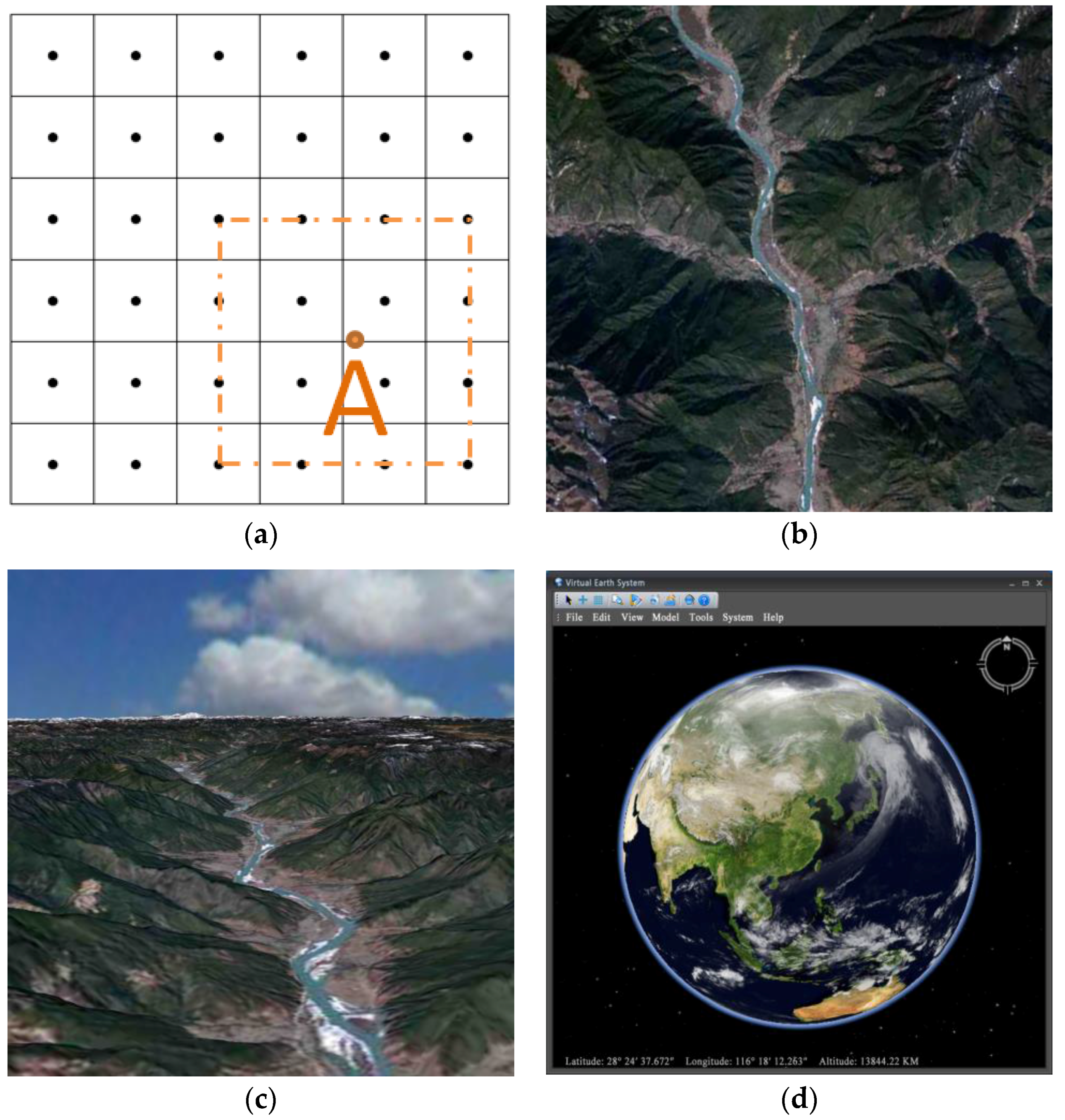
Figure 2.
(a) Description of regular grid DEM; (b) DOM data; (c) DEM and DOM data visualization; (d) Virtual globe platform.
Figure 2.
(a) Description of regular grid DEM; (b) DOM data; (c) DEM and DOM data visualization; (d) Virtual globe platform.
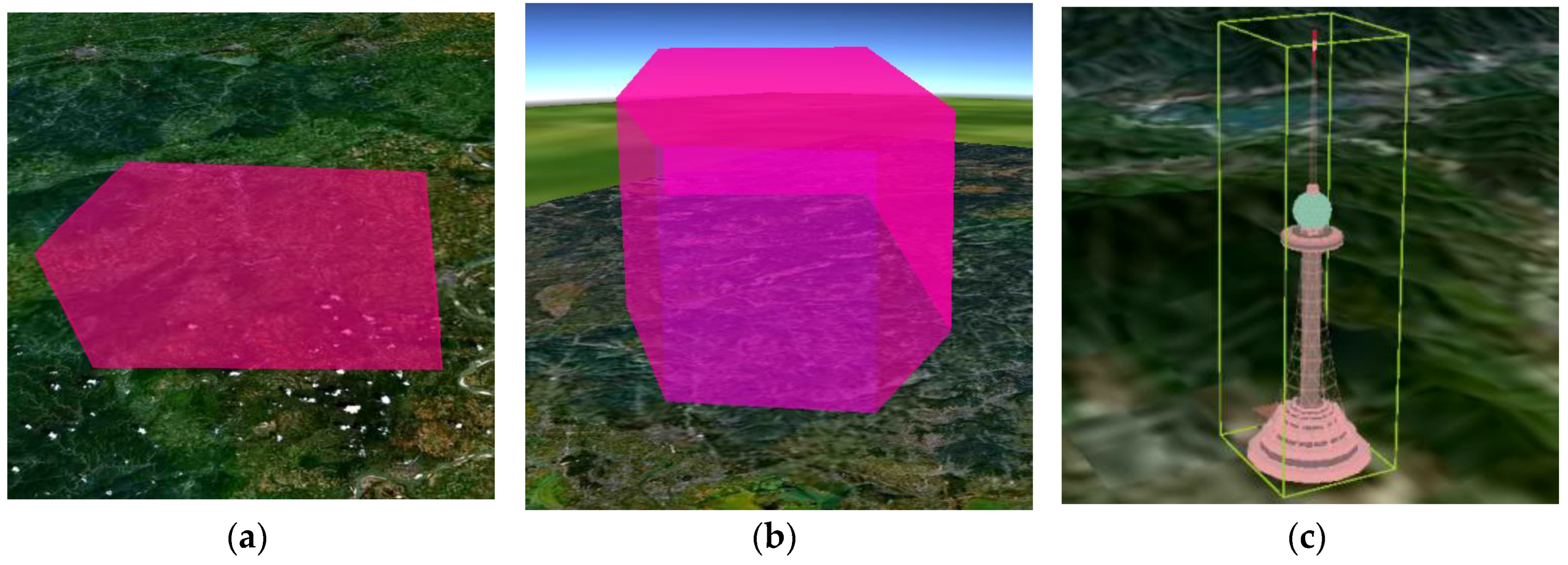
Figure 3.
(a) 2D No-fly zone; (b) 3D slowly hazardous weather model; (c) 3D threat model of a 500-m high TV tower described as {(114.655225, 23.269952), (114.658225, 23.269952), (114.658225, 23.272952), (114.655225, 23.272952), 500}.
Figure 3.
(a) 2D No-fly zone; (b) 3D slowly hazardous weather model; (c) 3D threat model of a 500-m high TV tower described as {(114.655225, 23.269952), (114.658225, 23.269952), (114.658225, 23.272952), (114.655225, 23.272952), 500}.
Figure 4.
(a) Model of a missile killing zone; (b) 3D visualization of a missile killing zone.
Figure 4.
(a) Model of a missile killing zone; (b) 3D visualization of a missile killing zone.
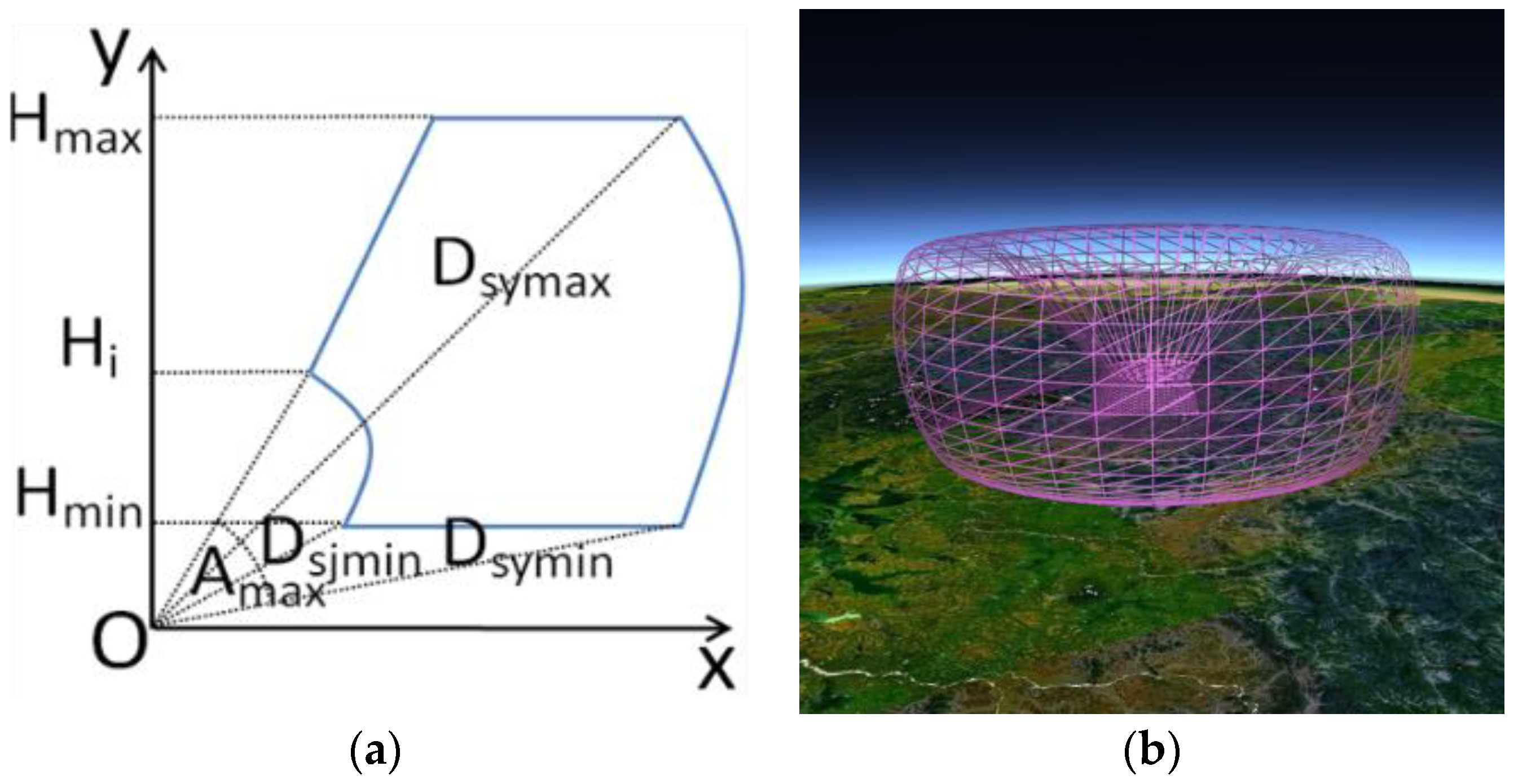
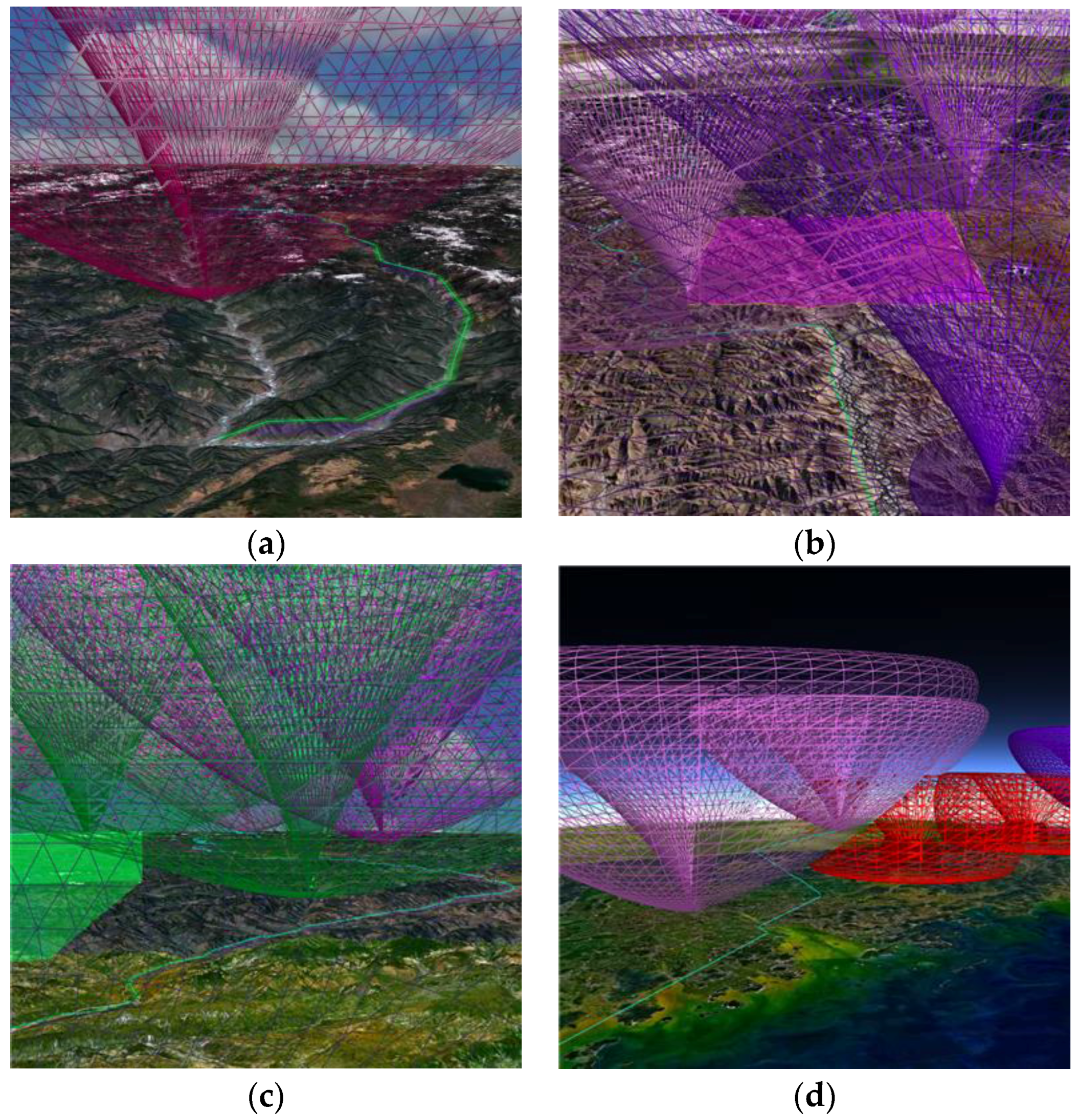
Figure 5.
(a) Radar signal propagation; (b) Earth curvature's influence.
Figure 5.
(a) Radar signal propagation; (b) Earth curvature's influence.
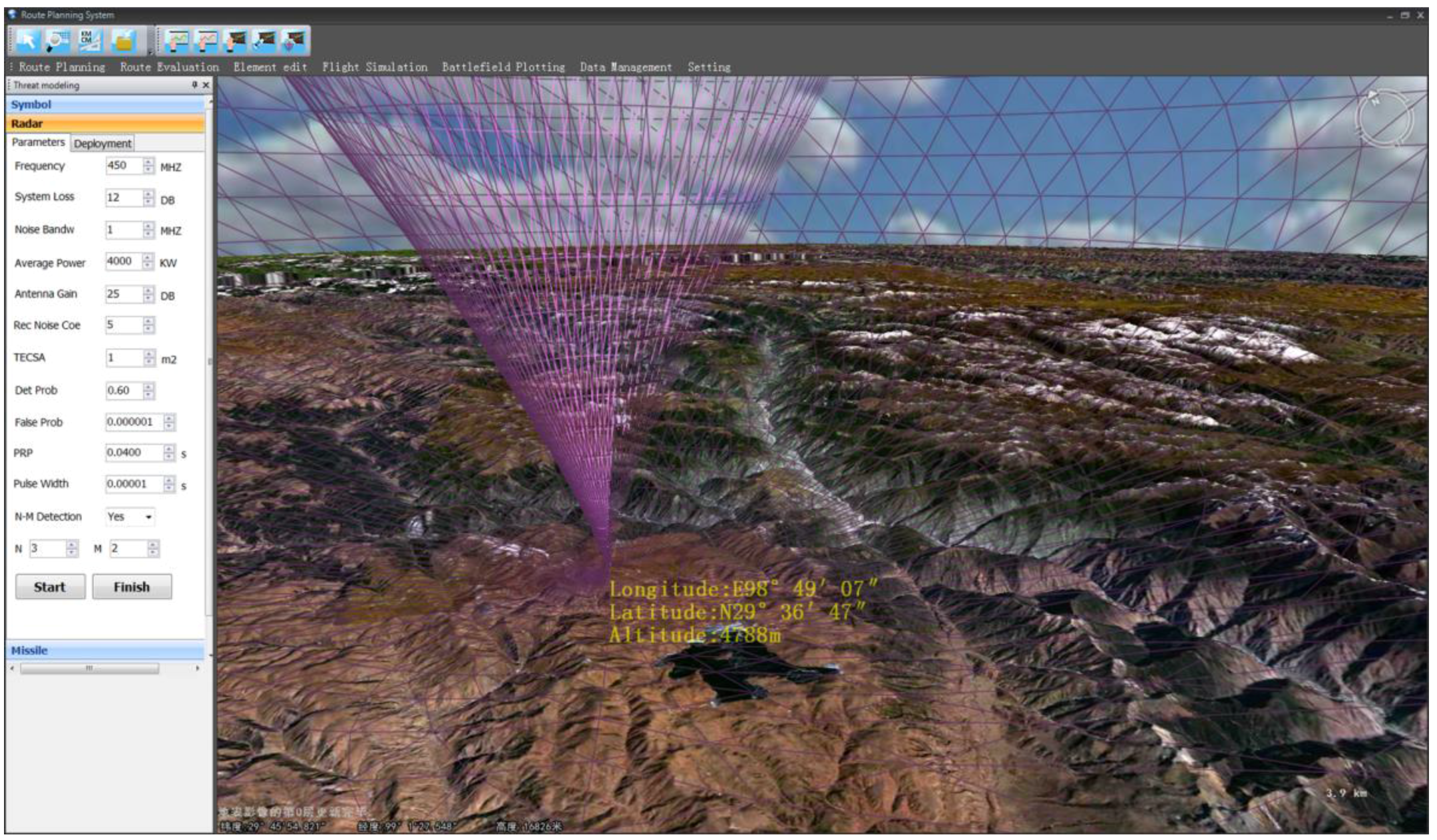
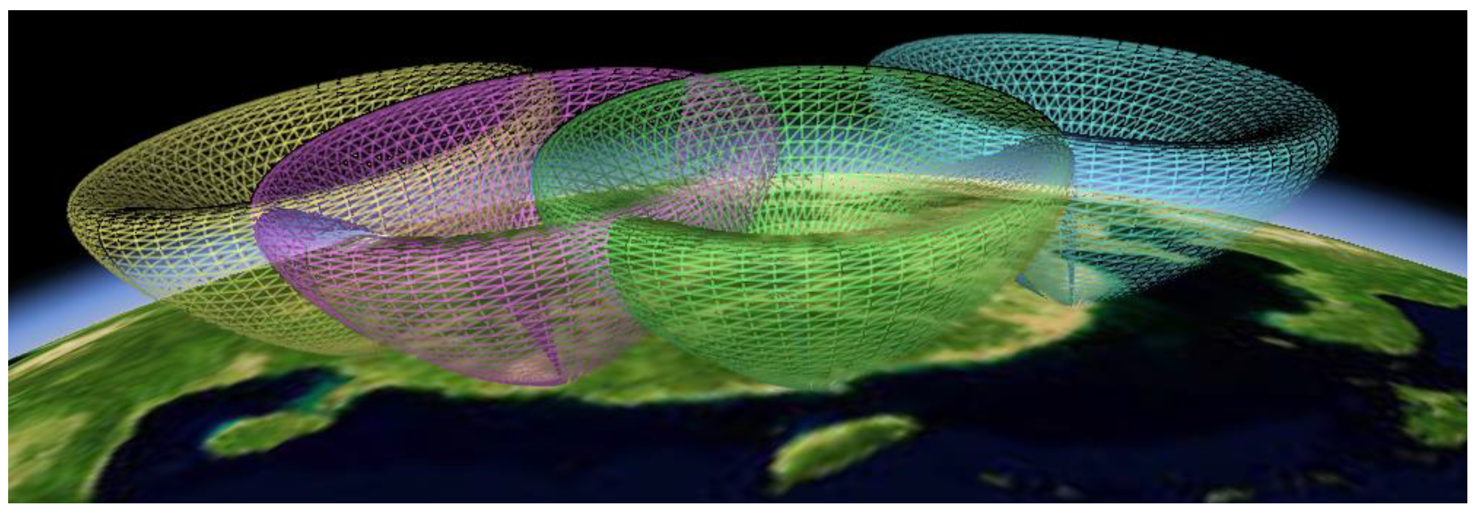
Figure 6.
Visualization of the radar networking coverage on the virtual globe.
Figure 6.
Visualization of the radar networking coverage on the virtual globe.
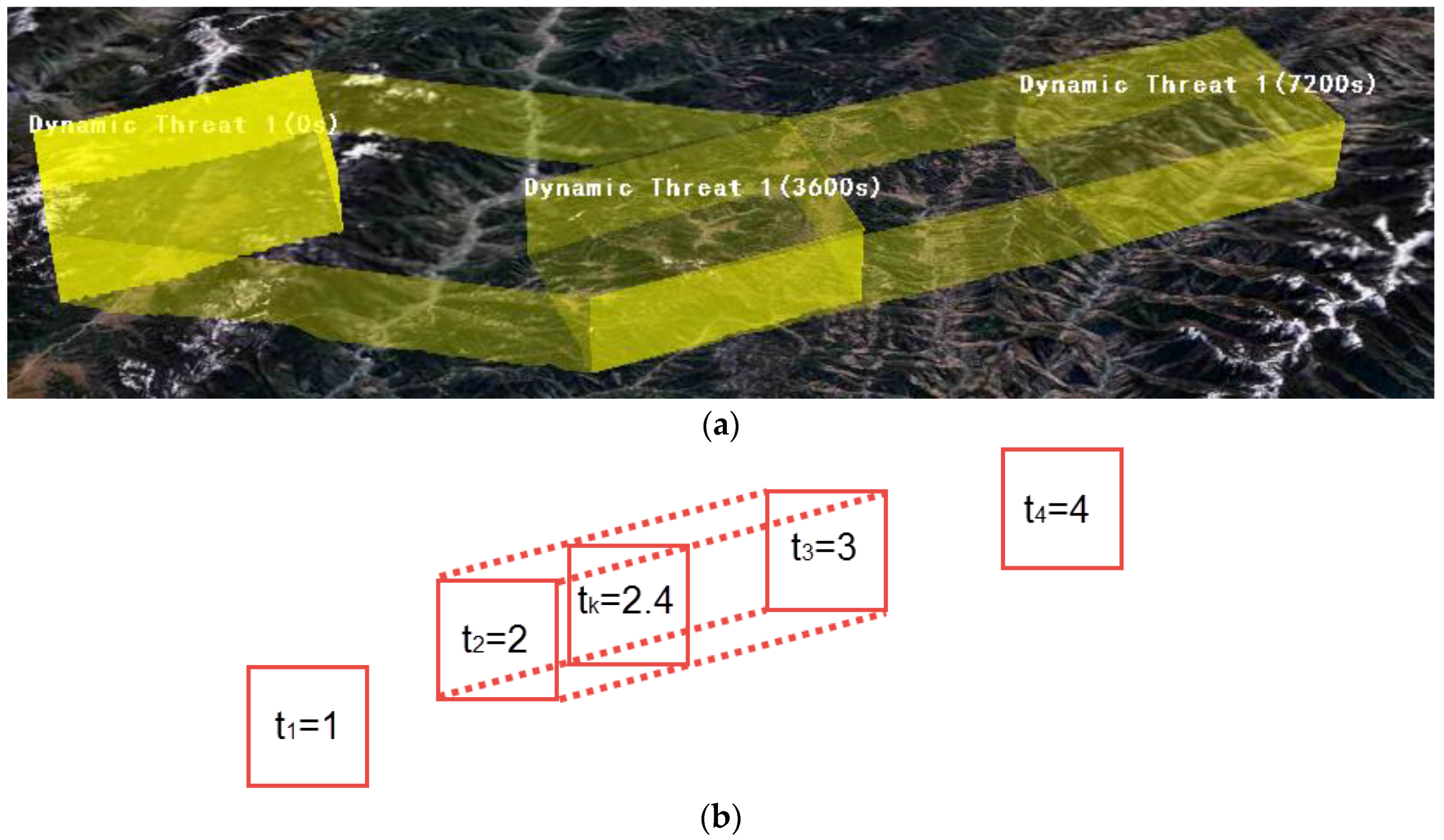
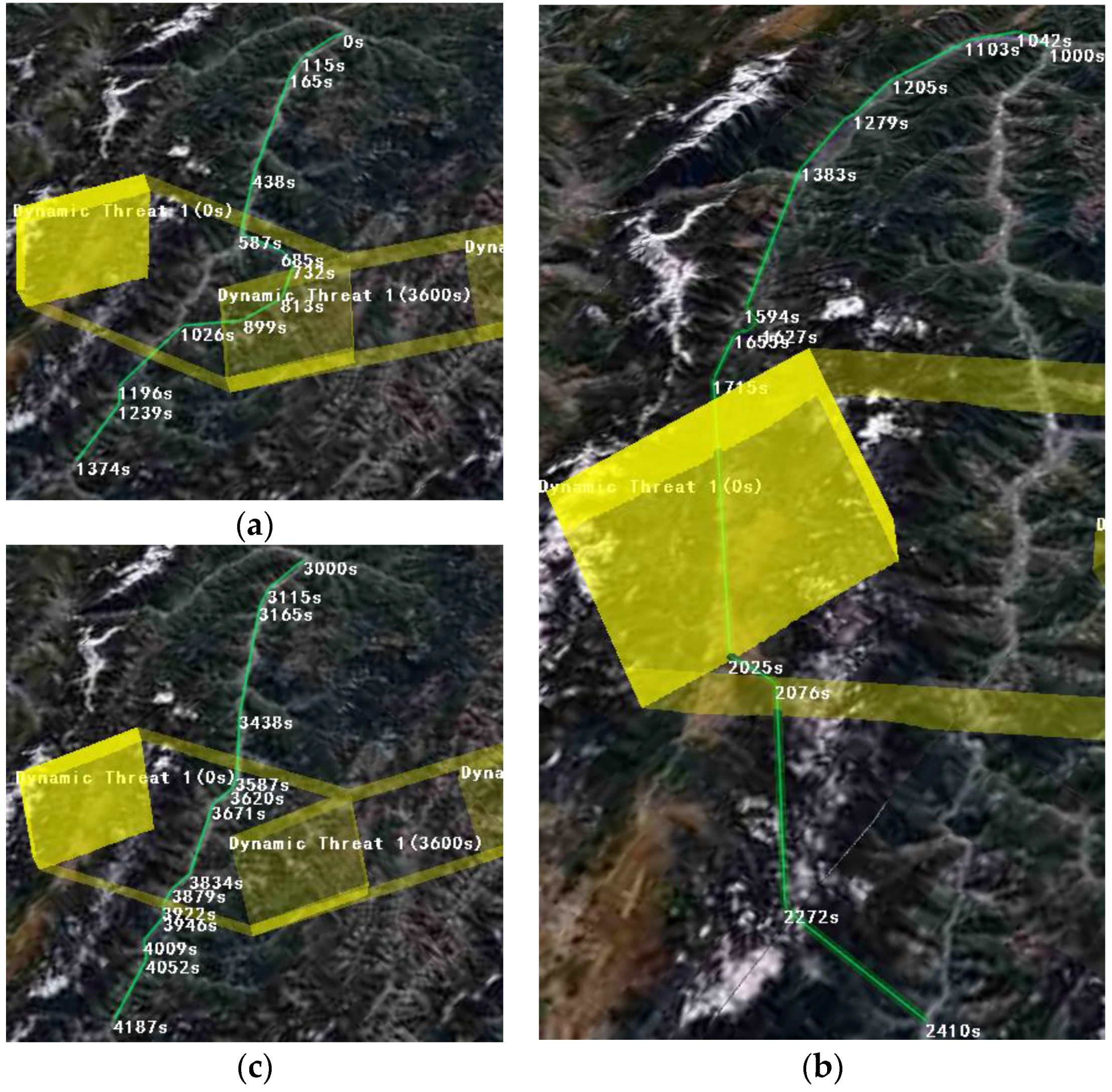
Figure 7.
Dynamic threat model. (a) There is a dynamic threat described as {{(99.94497, 27.60066), (99.859, 27.38197), (99.68604, 27.47941), (99.77718, 27.68262), 3000, 0 s}, {(99.54497, 27.40066), (99.459, 27.18197), (99.28604, 27.27941), (99.37718, 27.48262), (99.54497, 27.40066), 3000, 3600 s}, {(99.34497, 27.00066), (99.259, 26.78197), (99.08604, 26.87941), (99.17718, 27.08262), (99.34497, 27.00066), 3000, 7200 s}}; (b) Perform linear interpolation for the dynamic threat to obtain the threat status at any time.
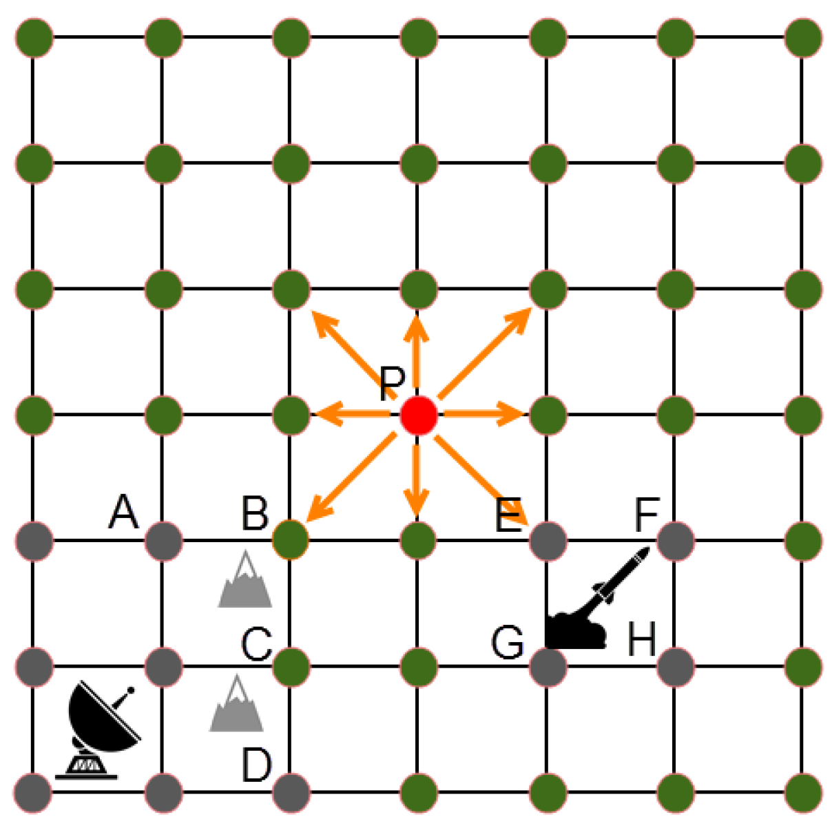
Figure 8.
Space division.
Figure 8.
Space division.
Figure 9.
(a) Route planning with threat; (b) Route planning with threat area expansion.
Figure 9.
(a) Route planning with threat; (b) Route planning with threat area expansion.
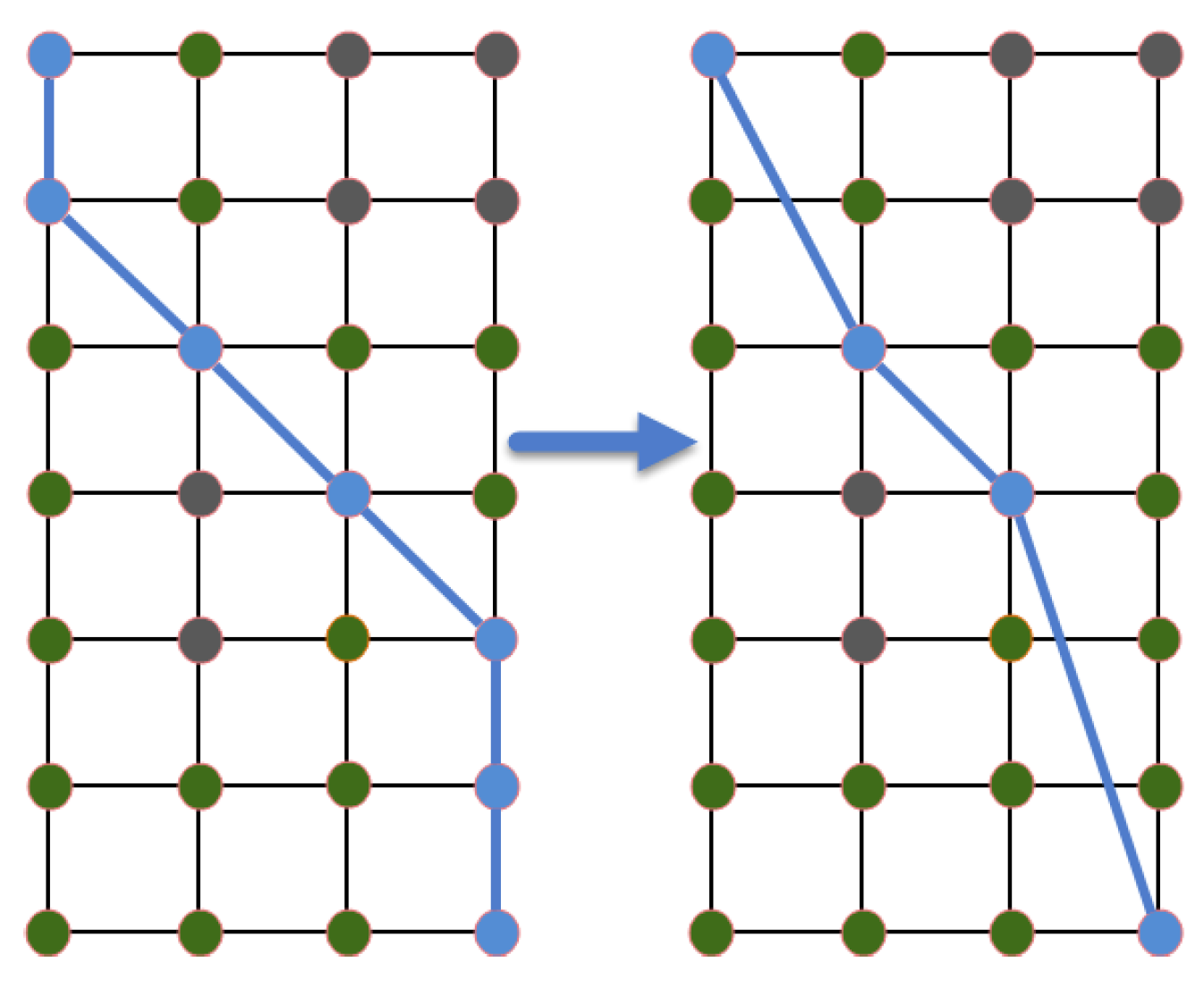
Figure 10.
Length changed before and after compression.
Figure 10.
Length changed before and after compression.
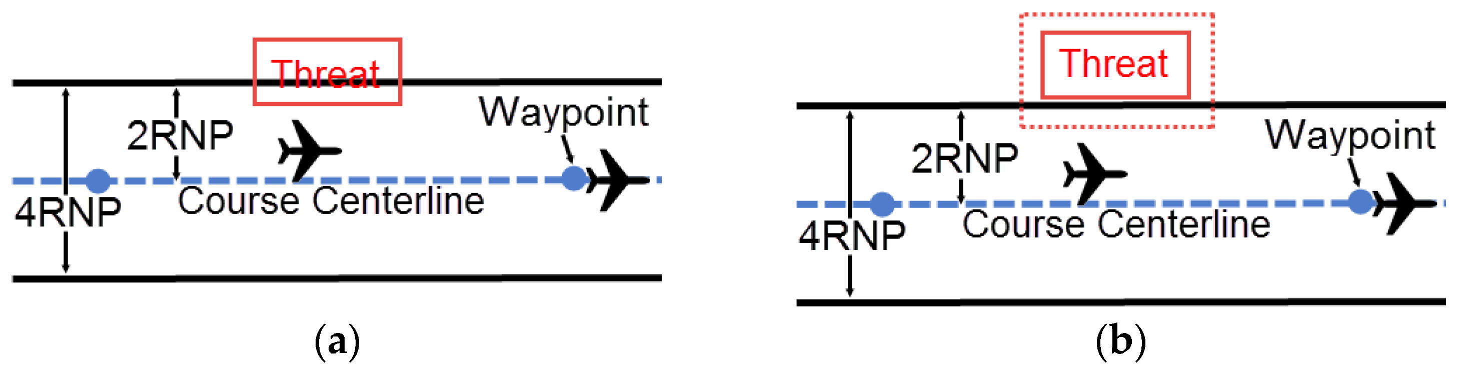
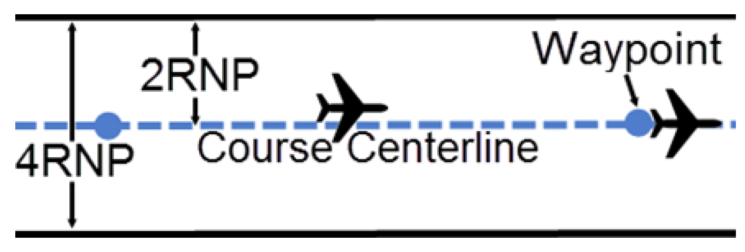
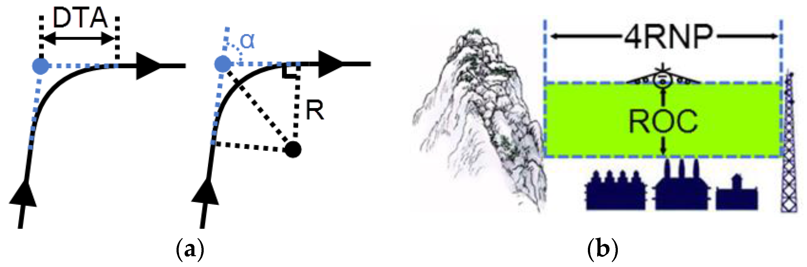
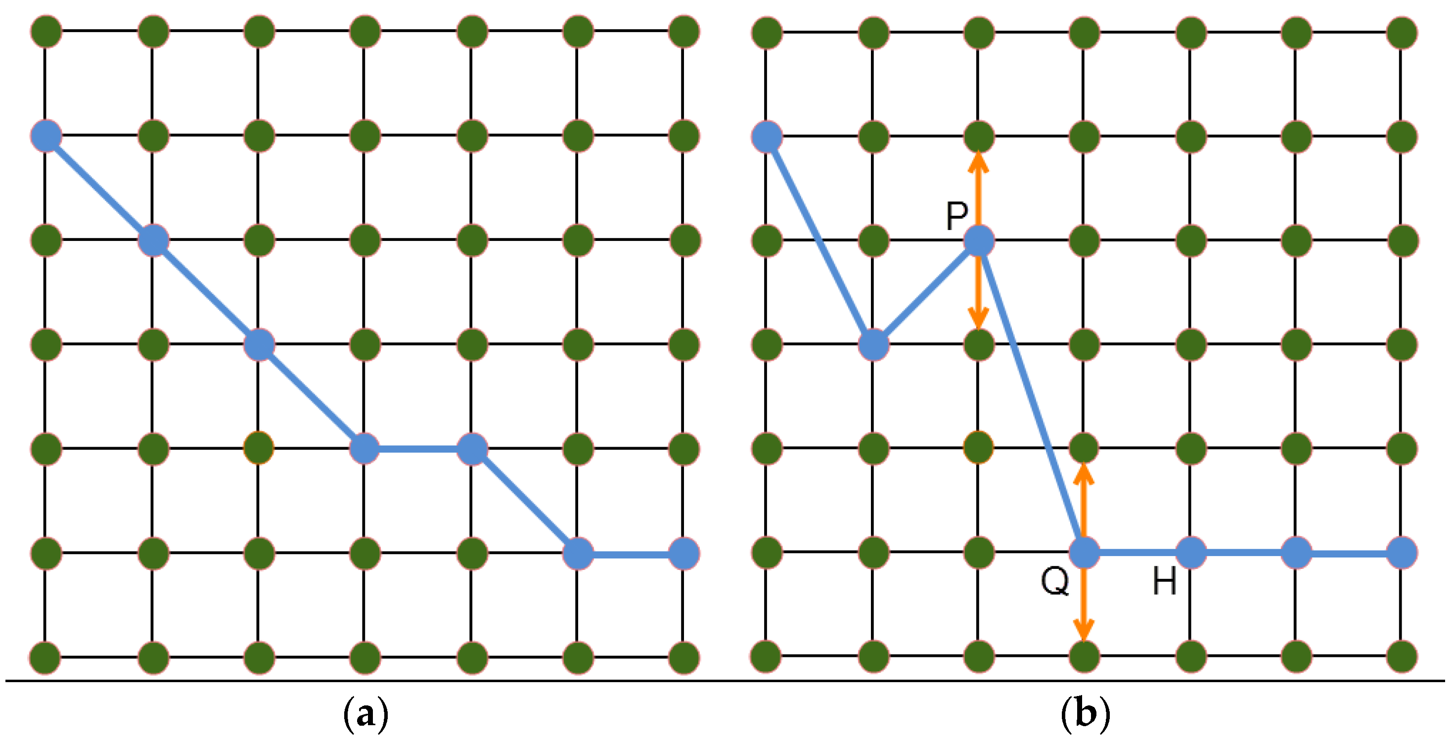
Figure 11.
(a) Distance of turn anticipation model; (b) Profile view for RNP segment width.
Figure 11.
(a) Distance of turn anticipation model; (b) Profile view for RNP segment width.
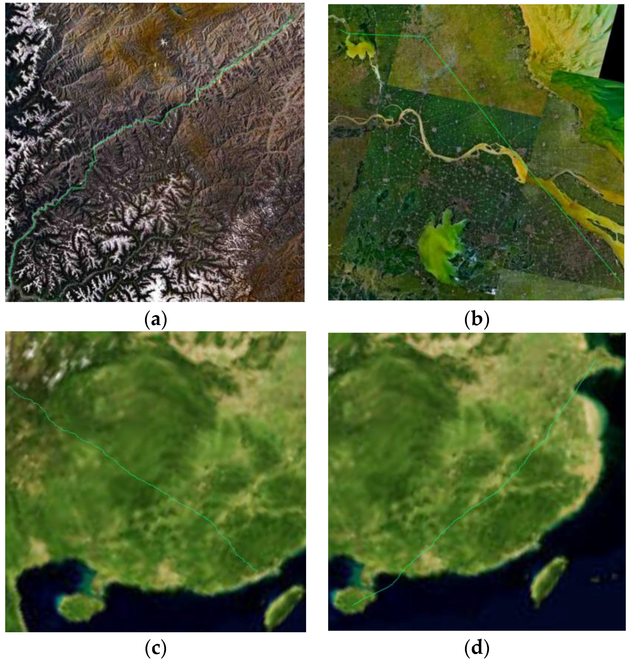
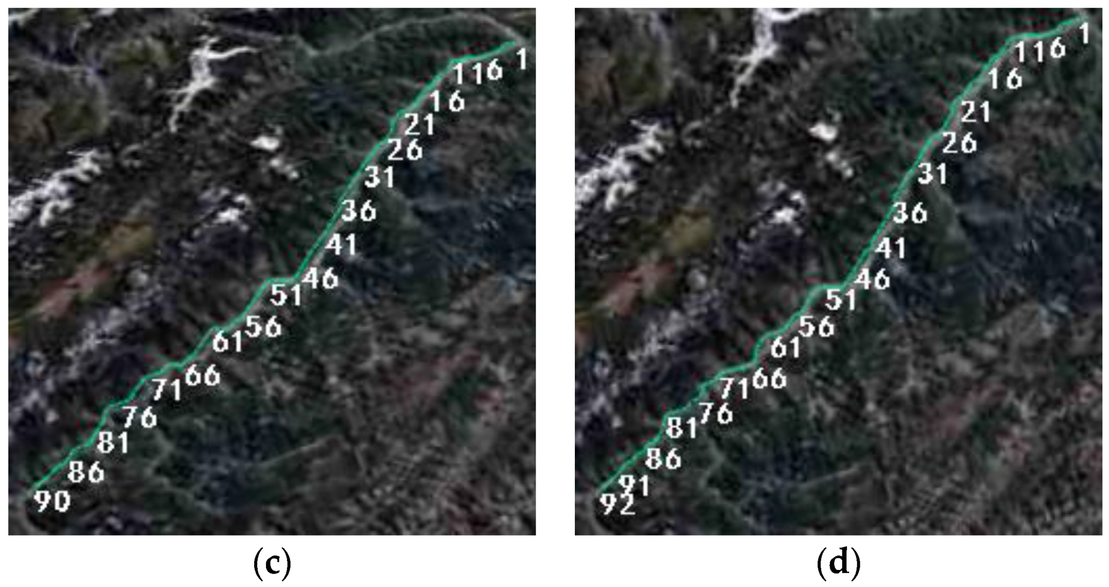
Figure 12.
Cartographic Map-1.
Figure 12.
Cartographic Map-1.
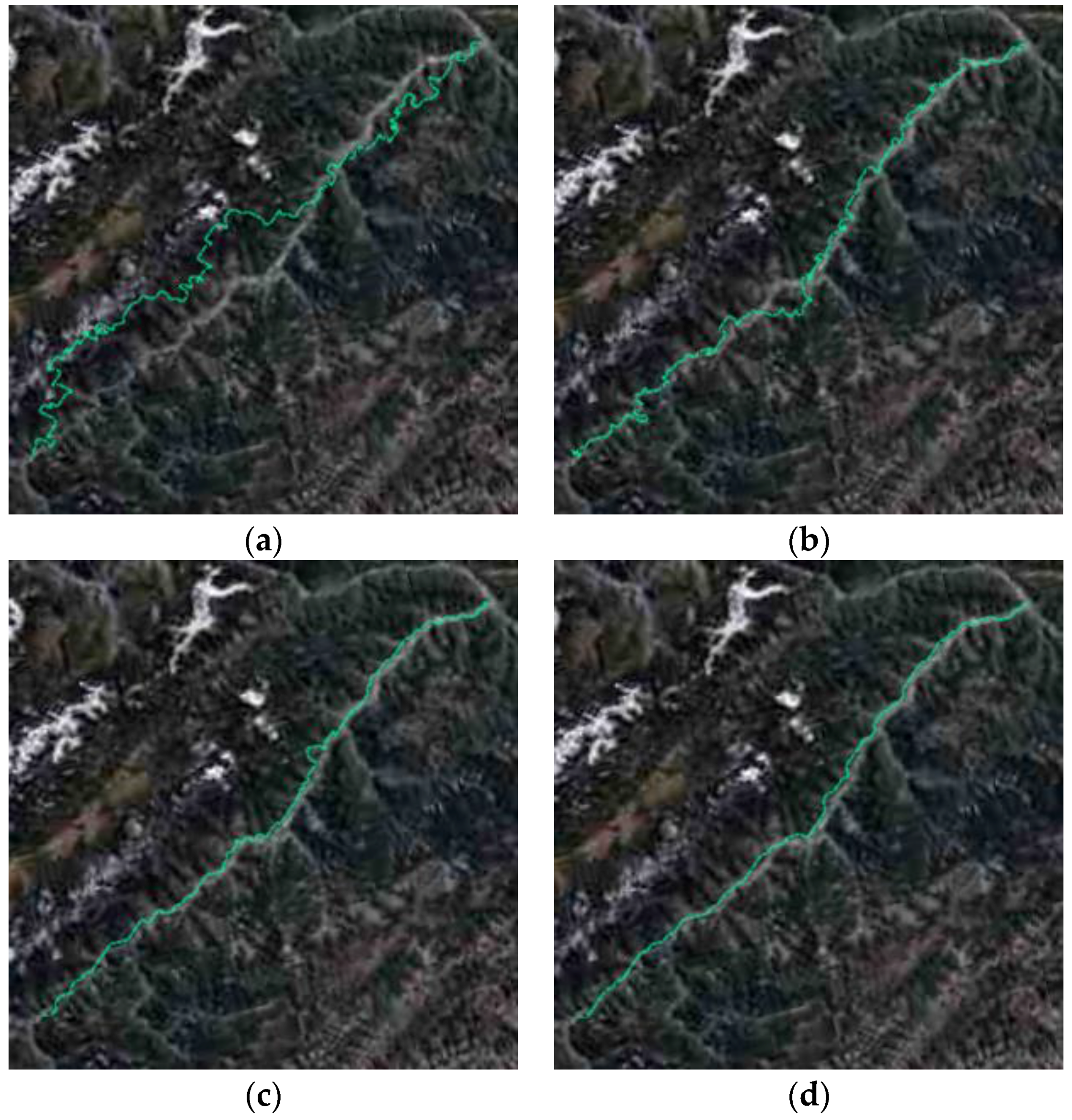
Figure 13.
Experiment results with different height cost coefficients . (a) ; (b) ; (c) ; (d) .
Figure 13.
Experiment results with different height cost coefficients . (a) ; (b) ; (c) ; (d) .
Figure 14.
Global optimal solutions for different iterations . (a) ; (b) ; (c) ; (d) .
Figure 14.
Global optimal solutions for different iterations . (a) ; (b) ; (c) ; (d) .
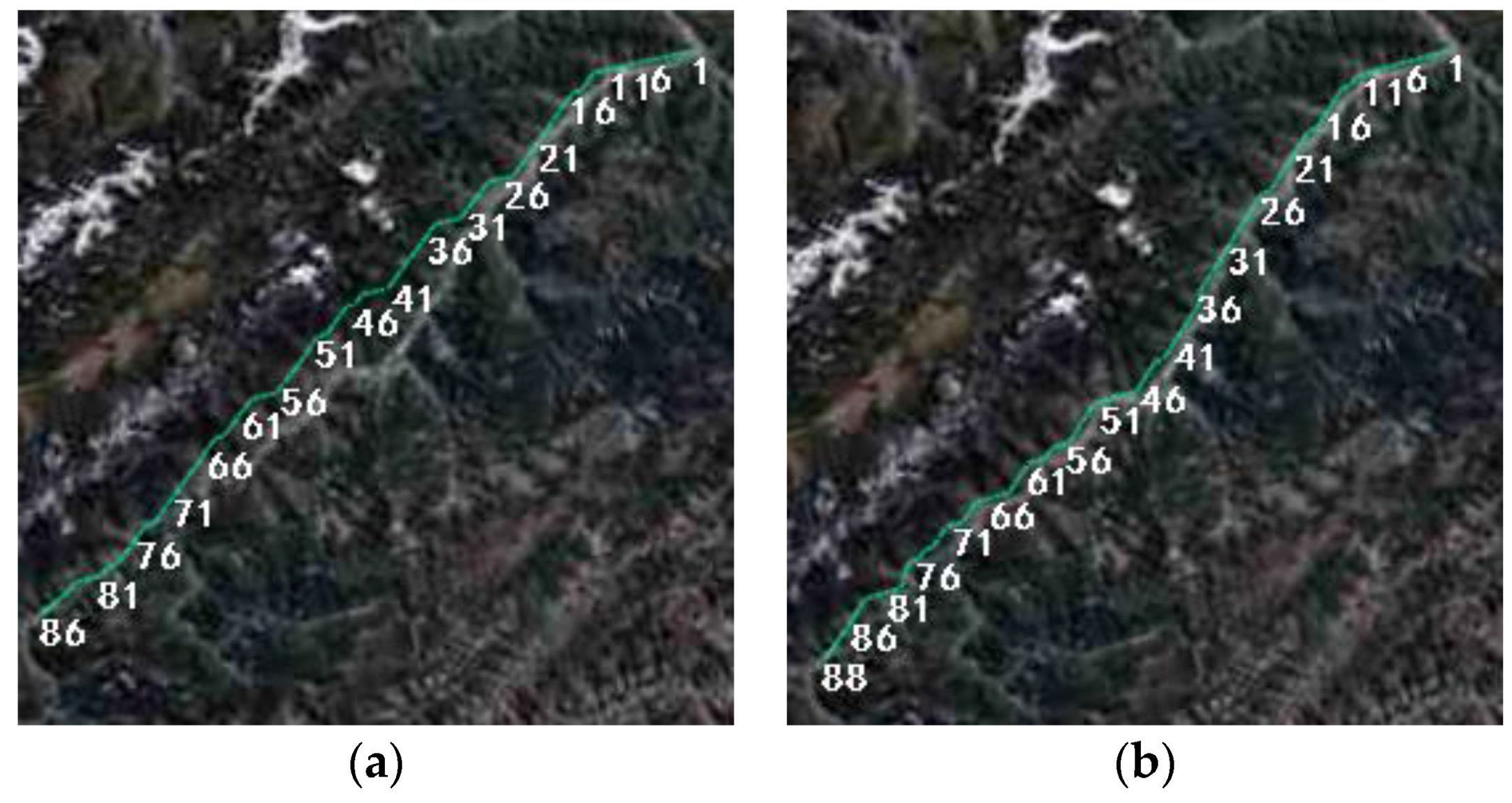
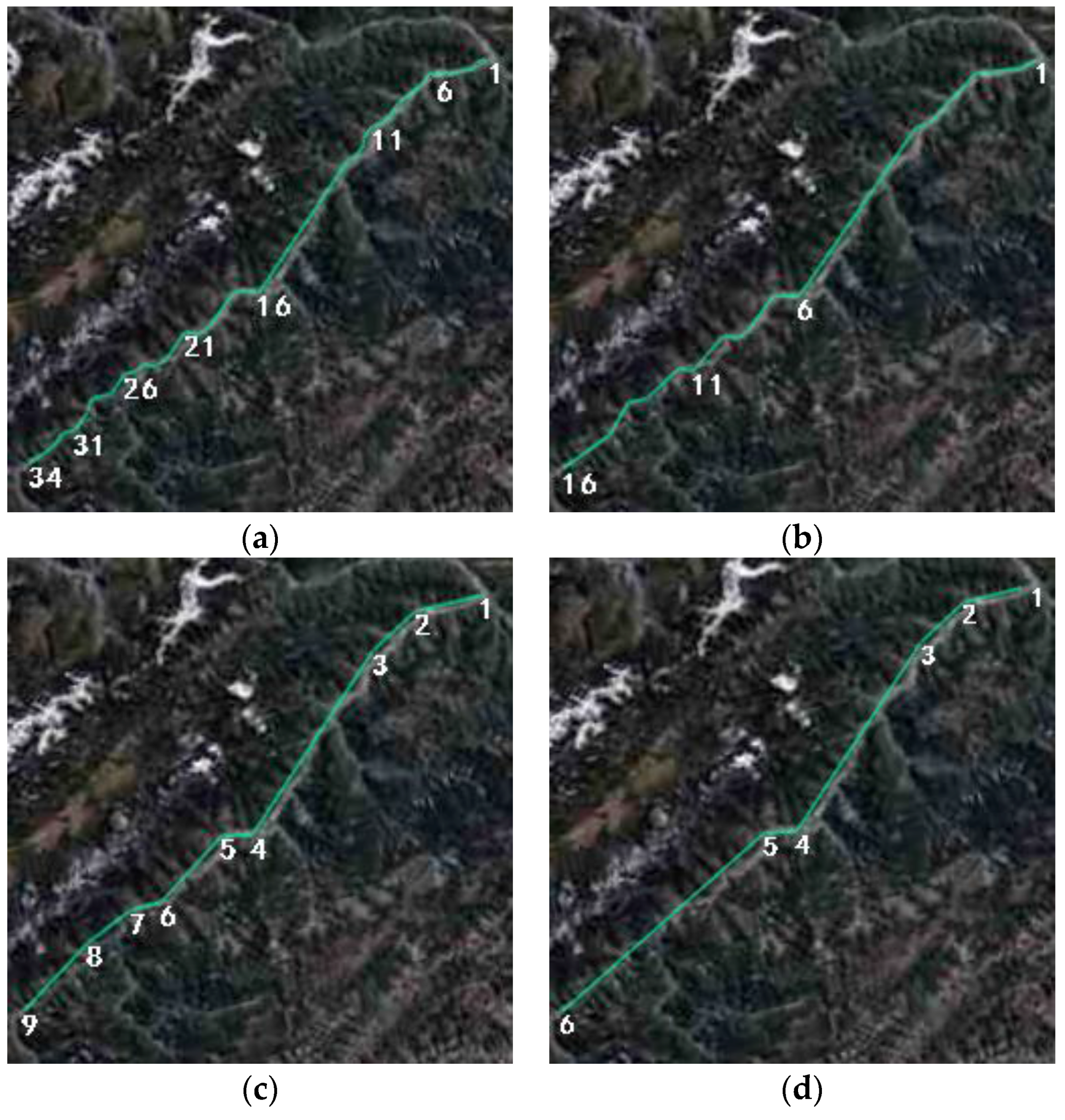
Figure 15.
Comparison results for different tolerances ϵ. (a) ϵ = 0.25 nmi; (b) ϵ = 0.50 nmi; (c) ϵ = 0.75 nmi; (d) ϵ = 1.00 nmi.
Figure 15.
Comparison results for different tolerances ϵ. (a) ϵ = 0.25 nmi; (b) ϵ = 0.50 nmi; (c) ϵ = 0.75 nmi; (d) ϵ = 1.00 nmi.
Figure 16.
Turning, falling and rising corner adjustment. (a) Before turning corner adjustment; (b) After turning corner adjustment.
Figure 16.
Turning, falling and rising corner adjustment. (a) Before turning corner adjustment; (b) After turning corner adjustment.
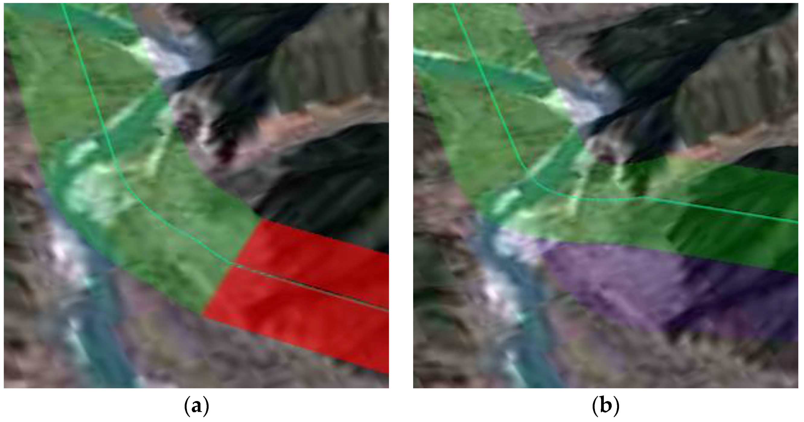
Figure 17.
Route optimization with route buffer areas. (a) Before height adjustment; (b) After height adjustment.
Figure 17.
Route optimization with route buffer areas. (a) Before height adjustment; (b) After height adjustment.
Figure 18.
Vertical flight path.
Figure 18.
Vertical flight path.
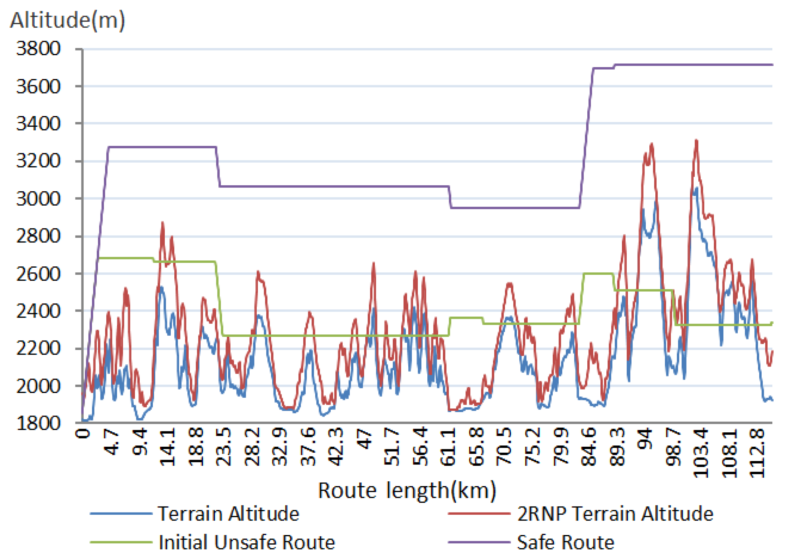
Figure 19.
(a) The optimal result for grid width = 0.005°, i, , terrain average altitude = 1905.73 m, and average altitude of the route after introducing the route buffer = 2698.37 m; (b,c) are local route details.
Figure 19.
(a) The optimal result for grid width = 0.005°, i, , terrain average altitude = 1905.73 m, and average altitude of the route after introducing the route buffer = 2698.37 m; (b,c) are local route details.
Figure 20.
The relationship between waypoint and node for different algorithms. (a) MACO, ACO, RAS, A*; (b) PSO, EA.
Figure 20.
The relationship between waypoint and node for different algorithms. (a) MACO, ACO, RAS, A*; (b) PSO, EA.
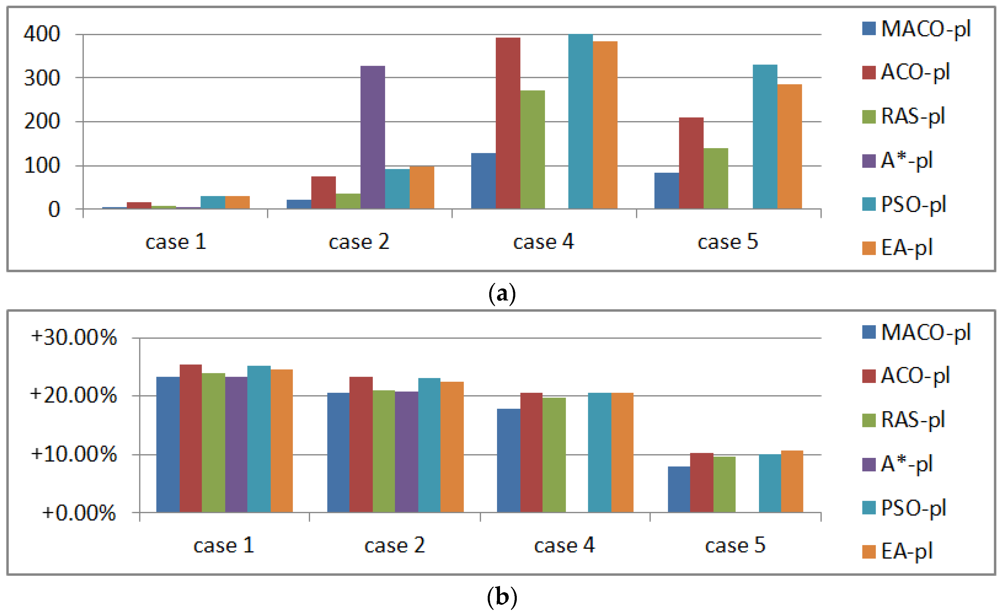
Figure 21.
Planning results of 1–5 coordinate groups. (a) Processing time (s); (b) Comparison with ; (c) Comparison with .
Figure 21.
Planning results of 1–5 coordinate groups. (a) Processing time (s); (b) Comparison with ; (c) Comparison with .
Figure 22.
Planning results of 2–5 coordinate groups using MACO-pl. (a) Coordinate group 2; (b) Coordinate group 3; (c) Coordinate group 4; (d) Coordinate group 5.
Figure 22.
Planning results of 2–5 coordinate groups using MACO-pl. (a) Coordinate group 2; (b) Coordinate group 3; (c) Coordinate group 4; (d) Coordinate group 5.
Figure 23.
Local details of the routes of 2–5 coordinate groups. (a) Coordinate group 2; (b) Coordinate group 3; (c) Coordinate group 4; (d) Coordinate group 5.
Figure 23.
Local details of the routes of 2–5 coordinate groups. (a) Coordinate group 2; (b) Coordinate group 3; (c) Coordinate group 4; (d) Coordinate group 5.
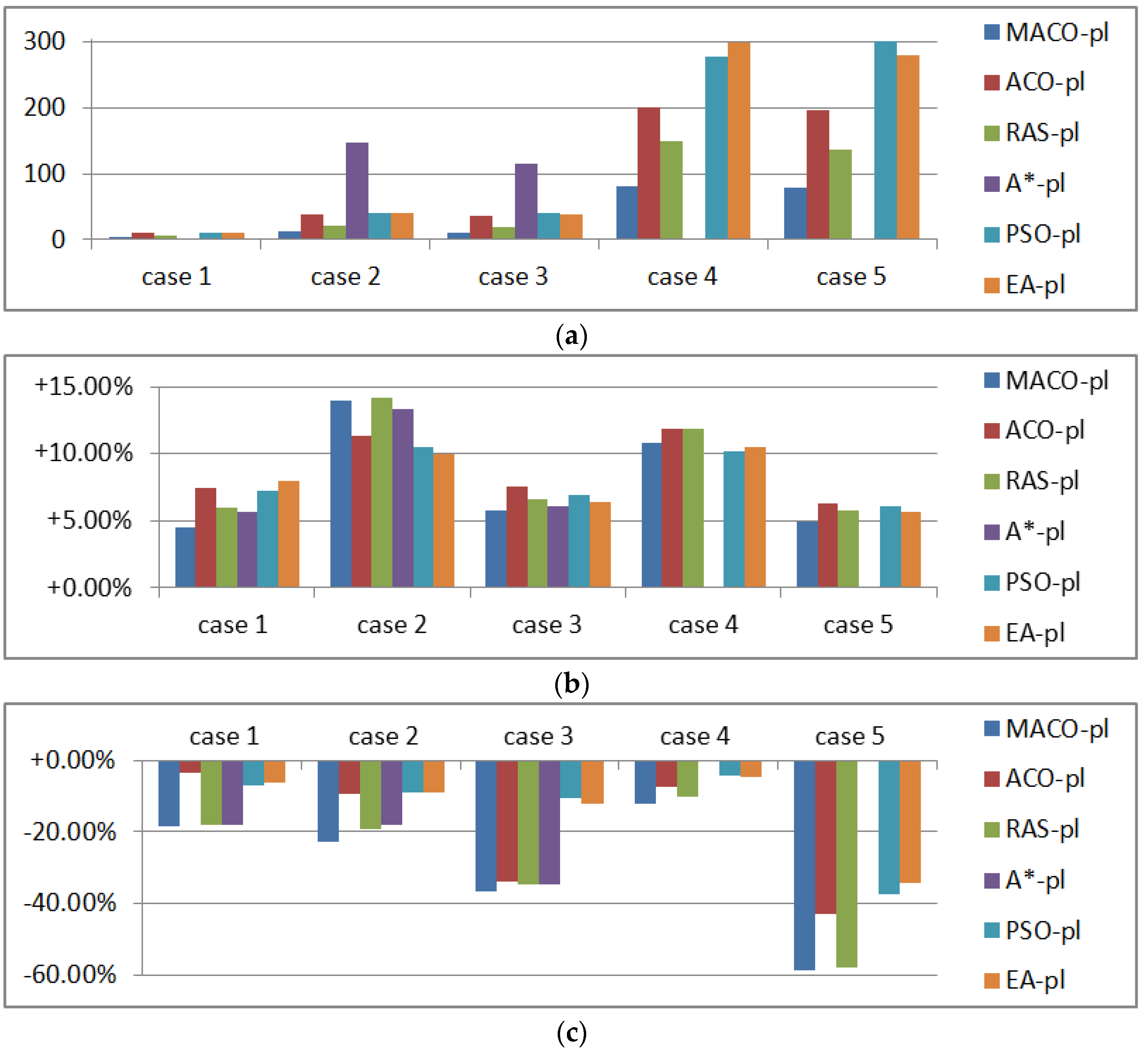
Figure 24.
Planning results under threat environments. (a) Processing time (s); (b) Comparison with ; (c) Comparison with .
Figure 24.
Planning results under threat environments. (a) Processing time (s); (b) Comparison with ; (c) Comparison with .
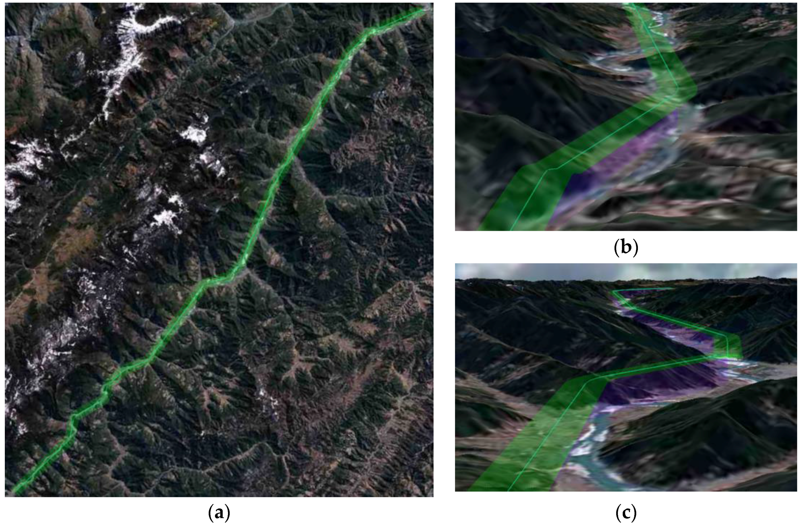
Figure 25.
Low altitude penetration routes using MACO-pl of different cases. (a) Case 1; (b) Case 2; (c) Case 4; (d) Case 5.
Figure 25.
Low altitude penetration routes using MACO-pl of different cases. (a) Case 1; (b) Case 2; (c) Case 4; (d) Case 5.
Figure 26.
The results of different start times under dynamic threats. (a) Start time = 0 s; (b) Start time = 1000 s; (c) Start time = 3000 s.
Figure 26.
The results of different start times under dynamic threats. (a) Start time = 0 s; (b) Start time = 1000 s; (c) Start time = 3000 s.
Table 1.
The UAV flight parameters.
Table 1.
The UAV flight parameters.
| (km/h) | (km/h) | Maximum Lifting Angle | (m) | RNP (nmi) | Turning Fix |
|---|
| 350 | 0 | 20° | 400 | 0.25 | Fly-by Fix |
Table 2.
Experimental coordinate groups.
Table 2.
Experimental coordinate groups.
| Serial Number | Start Point | End Point | | |
|---|
| | (km) | (m) |
|---|
| 1 | 99.96463° | 99.43347° | 110.613 | 2339.93 |
| 26.88202° | 27.75616° |
| 1819.58 m | 2530.68 m |
| 2 | 90.86051° | 94.46516° | 350.051 | 4492.95 |
| 29.30996° | 29.42218° |
| 3573.99 m | 2951.15 m |
| 3 | 121.84255° | 119.05692° | 342.512 | 4.49 |
| 30.98066° | 32.95193° |
| 21.51 m | 14.17 m |
| 4 | 99.44990° | 118.45611° | 1909.435 | 1186.37 |
| 27.81014° | 25.09058° |
| 1723.22 m | 397.35 m |
| 5 | 109.78029° | 120.41494° | 2259.830 | 203.71 |
| 18.85893° | 37.01404° |
| 445.07 m | 132.31 m |
Table 3.
Comparison results for different coefficients.
Table 3.
Comparison results for different coefficients.
| Coefficients () | Planning Time (s) | (km) | (m) | Waypoint Number | Compared with | Compared with |
|---|
| 0 | 1.01 | 118.428 | 2488.07 | 86 | +7.07% | +6.33% |
| 0.5 | 1.09 | 119.074 | 2351.98 | 87 | +7.65% | +0.51% |
| 1 | 1.20 | 119.924 | 2152.15 | 88 | +8.42% | −8.03% |
| 1.5 | 1.29 | 119.995 | 2138.84 | 89 | +8.48% | −8.59% |
| 2 | 1.37 | 120.617 | 2058.38 | 90 | +9.04% | −12.03% |
| 2.5 | 1.55 | 123.085 | 2028.94 | 92 | +11.28% | −13.29% |
| 3 | N/A | | | | | |
Table 4.
Comparison results for different tolerances.
Table 4.
Comparison results for different tolerances.
| (nmi) | (km) | (m) | Waypoint Number | Compared with | Compared with |
|---|
| 0.25 | 120.129 | 2063.33 | 34 | +8.60% | −11.82% |
| 0.50 | 117.172 | 2060.58 | 16 | +5.93% | −11.94% |
| 0.75 | 116.003 | 2141.67 | 9 | +4.87% | −8.47% |
| 1.00 | 115.061 | 2120.13 | 6 | +4.02% | −9.39% |
Table 5.
Comparison of results with different granularity.
Table 5.
Comparison of results with different granularity.
| Grid Width | (nmi) | Processing Time (s) | (km) | (m) | Compared with | Compared with |
|---|
| 0.007° | 0.75 | 2.15 | 115.117 | 1975.70 | +4.07% | −15.57% |
| 0.007° | 0.50 | 2.15 | 116.899 | 1947.84 | +5.68% | −16.76% |
| 0.006° | 0.75 | 2.73 | 114.404 | 1979.44 | +3.43% | −15.41% |
| 0.006° | 0.50 | 2.73 | 117.060 | 1953.05 | +5.83% | −16.53% |
| 0.005° | 0.75 | 3.21 | 114.086 | 1942.91 | +3.14% | −16.97% |
| 0.005° | 0.50 | 3.21 | 115.603 | 1905.73 | +4.51% | −18.56% |
| 0.004° | 0.75 | 4.24 | 114.403 | 1955.89 | +3.43% | −16.41% |
| 0.004° | 0.50 | 4.24 | 115.523 | 1923.16 | +4.44% | −17.81% |
| 0.003° | 0.75 | 6.18 | 114.498 | 1961.64 | +3.51% | −16.17% |
| 0.003° | 0.50 | 6.18 | 115.300 | 1925.10 | +4.24% | −17.73% |
| 0.002° | 0.75 | 7.37 | 115.033 | 1973.27 | +4.00% | −15.67% |
| 0.002° | 0.50 | 7.37 | 115.711 | 1961.85 | +4.61% | −16.16% |
Table 6.
Planning results of 1–5 coordinate groups.
Table 6.
Planning results of 1–5 coordinate groups.
| Serial Number | Method | Processing Time (s) | (km) | (m) | Compared with | Compared with |
|---|
| 1 | MACO-pl | 3.21 | 115.603 | 1905.73 | +4.51% | −18.56% |
| 1 | ACO-pl | 10.07 | 118.831 | 2262.32 | +7.43% | −3.32% |
| 1 | RAS-pl | 5.66 | 117.267 | 1914.28 | +6.02% | −18.19% |
| 1 | A*-pl | 2.16 | 116.875 | 1916.29 | +5.66% | −18.10% |
| 1 | PSO-pl | 9.78 | 118.679 | 2177.42 | +7.29% | −6.94% |
| 1 | EA-pl | 10.84 | 119.441 | 2190.32 | +7.98% | −6.39% |
| 2 | MACO-pl | 12.39 | 398.782 | 3471.04 | +13.92% | −22.74% |
| 2 | ACO-pl | 38.48 | 389.907 | 4074.93 | +11.39% | −9.30% |
| 2 | RAS-pl | 20.40 | 399.823 | 3623.61 | +14.22% | −19.35% |
| 2 | A*-pl | 148.14 | 396.934 | 3681.73 | +13.39% | −18.05% |
| 2 | PSO-pl | 40.02 | 386.679 | 4081.56 | +10.46% | −9.15% |
| 2 | EA-pl | 41.28 | 385.041 | 4094.39 | +10.00% | −8.87% |
| 3 | MACO-pl | 10.96 | 362.433 | 2.85 | +5.82% | −36.53% |
| 3 | ACO-pl | 36.42 | 368.345 | 2.98 | +7.54% | −33.63% |
| 3 | RAS-pl | 18.67 | 365.184 | 2.93 | +6.62% | −34.74% |
| 3 | A*-pl | 116.23 | 363.245 | 2.94 | +6.05% | −34.52% |
| 3 | PSO-pl | 39.57 | 366.176 | 4.01 | +6.91% | −10.69% |
| 3 | EA-pl | 38.95 | 364.504 | 3.95 | +6.42% | −12.03% |
| 4 | MACO-pl | 80.12 | 2115.333 | 1043.90 | +10.78% | −12.01% |
| 4 | ACO-pl | 201.15 | 2135.830 | 1097.04 | +11.85% | −7.53% |
| 4 | RAS-pl | 149.98 | 2136.106 | 1063.77 | +11.87% | −10.33% |
| 4 | A*-pl | N/A | | | | |
| 4 | PSO-pl | 278.26 | 2104.857 | 1137.25 | +10.23% | −4.14% |
| 4 | EA-pl | 299.38 | 2109.891 | 1131.32 | +10.50% | −4.64% |
| 5 | MACO-pl | 78.84 | 2371.012 | 84.59 | +4.92% | −58.48% |
| 5 | ACO-pl | 197.43 | 2401.023 | 116.56 | +6.25% | −42.78% |
| 5 | RAS-pl | 136.01 | 2390.174 | 85.99 | +5.76% | −57.79% |
| 5 | A*-pl | N/A | | | | |
| 5 | PSO-pl | 301.44 | 2398.322 | 127.76 | +6.13% | −37.28% |
| 5 | EA-pl | 279.64 | 2388.459 | 134.31 | +5.69% | −34.07% |
Table 7.
Planning results in threat environments.
Table 7.
Planning results in threat environments.
| Serial Number | Method | Processing Time (s) | (km) | (m) | (km) | Compared with | Compared with |
|---|
| 1 | MACO-pl | 5.63 | 136.480 | 2725.64 | 0 | +23.39% | +16.48% |
| 1 | ACO-pl | 17.02 | 138.737 | 2870.48 | 0 | +25.43% | +22.67% |
| 1 | RAS-pl | 9.39 | 137.158 | 2757.80 | 0 | +24.00% | +17.86% |
| 1 | A*-pl | 5.27 | 136.497 | 2789.72 | 0 | +23.40% | +19.22% |
| 1 | PSO-pl | 29.84 | 138.528 | 2955.42 | 0 | +25.24% | +26.30% |
| 1 | EA-pl | 31.15 | 137.917 | 2918.81 | 0 | +24.68% | +24.74% |
| 2 | MACO-pl | 20.85 | 421.922 | 4379.01 | 0 | +20.53% | −2.54% |
| 2 | ACO-pl | 75.35 | 431.943 | 4687.66 | 0 | +23.39% | +4.33% |
| 2 | RAS-pl | 37.28 | 423.871 | 4470.49 | 0 | +21.09% | −0.50% |
| 2 | A*-pl | 326.92 | 422.775 | 4450.11 | 0 | +20.78% | −0.95% |
| 2 | PSO-pl | 91.49 | 430.563 | 4716.47 | 0 | +23.00% | +4.97% |
| 2 | EA-pl | 99.02 | 428.719 | 4671.99 | 0 | +22.47% | +3.98% |
| 4 | MACO-pl | 127.39 | 2250.836 | 1086.37 | 0 | +17.88% | −8.43% |
| 4 | ACO-pl | 391.50 | 2301.760 | 1143.74 | 0 | +20.55% | −3.59% |
| 4 | RAS-pl | 271.98 | 2284.541 | 1109.44 | 0 | +19.64% | −6.49% |
| 4 | A*-pl | N/A | | | | | |
| 4 | PSO-pl | 401.32 | 2304.283 | 1217.07 | 0 | +20.68% | +2.59% |
| 4 | EA-pl | 384.56 | 2300.575 | 1203.64 | 0 | +20.48% | +1.46% |
| 5 | MACO-pl | 84.26 | 2438.912 | 86.22 | 0 | +7.92% | −57.68% |
| 5 | ACO-pl | 209.92 | 2494.026 | 119.14 | 0 | +10.36% | −41.51% |
| 5 | RAS-pl | 140.15 | 2477.678 | 86.85 | 0 | +9.64% | −57.37% |
| 5 | A*-pl | N/A | | | | | |
| 5 | PSO-pl | 329.48 | 2489.205 | 129.49 | 0 | +10.15% | −36.43% |
| 5 | EA-pl | 286.77 | 2503.418 | 136.61 | 0 | +10.78% | −32.94% |
Table 8.
The results of different start times under dynamic threats.
Table 8.
The results of different start times under dynamic threats.
| Start Time (s) | Planning Time (s) | (km) | (m) | Compared with | Compared with |
|---|
| 0 | 10.01 | 133.850 | 2112.65 | +21.01% | −9.71% |
| 1000 | 12.14 | 135.633 | 2724.18 | +22.62% | +16.42% |
| 2000 | 12.89 | 136.204 | 2725.49 | +23.14% | +16.48% |
| 3000 | 9.49 | 115.377 | 1906.71 | +4.31% | −18.51% |


