
Landslide Susceptibility Mapping Based on Particle Swarm Optimization of Multiple Kernel Relevance Vector Machines: Case of a Low Hill Area in Sichuan Province, China


Abstract
:1. Introduction
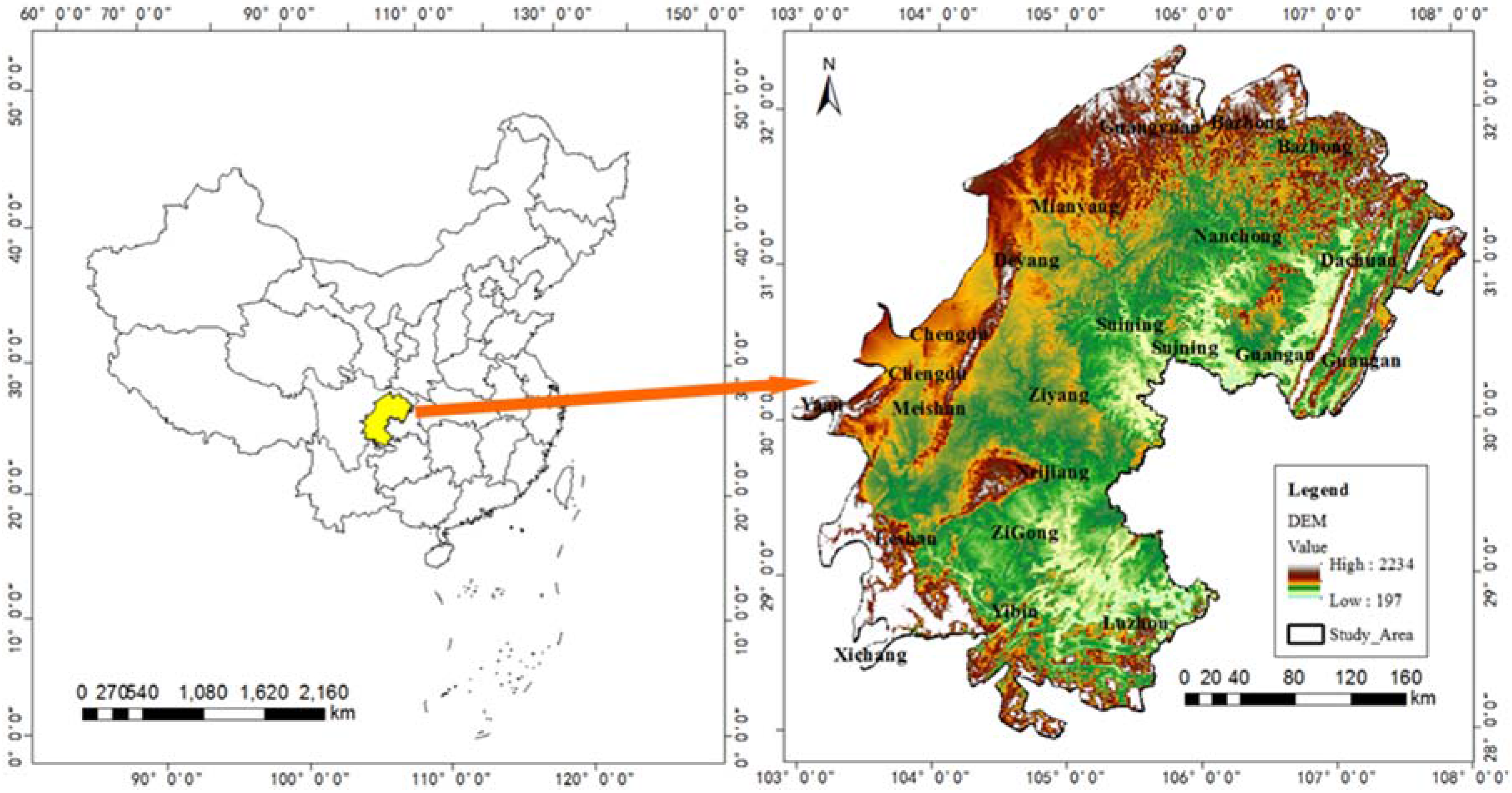
2. Study Area
3. Methods
3.1. Relevance Vector Machine
3.2. Multiple Kernel RVM
3.3. Particle Swarm Optimization
- (1)
- When , the fitness of these particles is closer to the optimal solution (the lowest error rate). Therefore, set a low inertia weight value to speed up local convergence.
- (2)
- When and , these particles are relatively far from the best fitness, which can be improved by the cloud model.The expectation of the cloud model is .The entropy can be calculated using the distance of the expectation and : .In addition, the hyper entropy was set using .The value of the inertia weight can be described as:According to “3En” rules, the control parameters and were set to 3 and 10 [24]. “normrnd” generates normally distributed data.
- (3)
- When , these particles need a higher inertia weight to improve the global search capability.
3.4. PSO-MKRVM
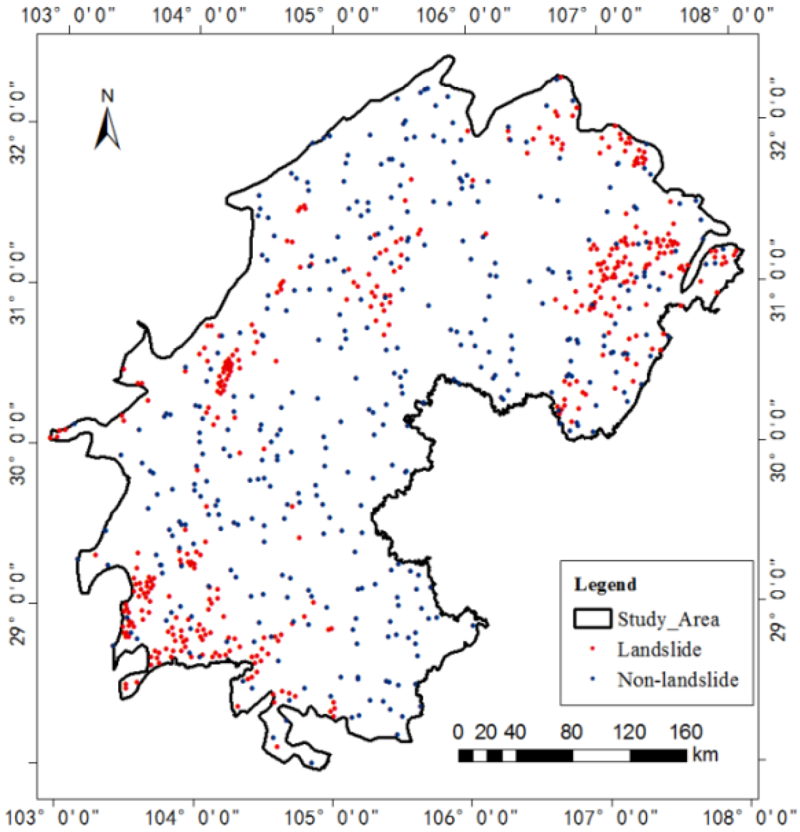
4. Data
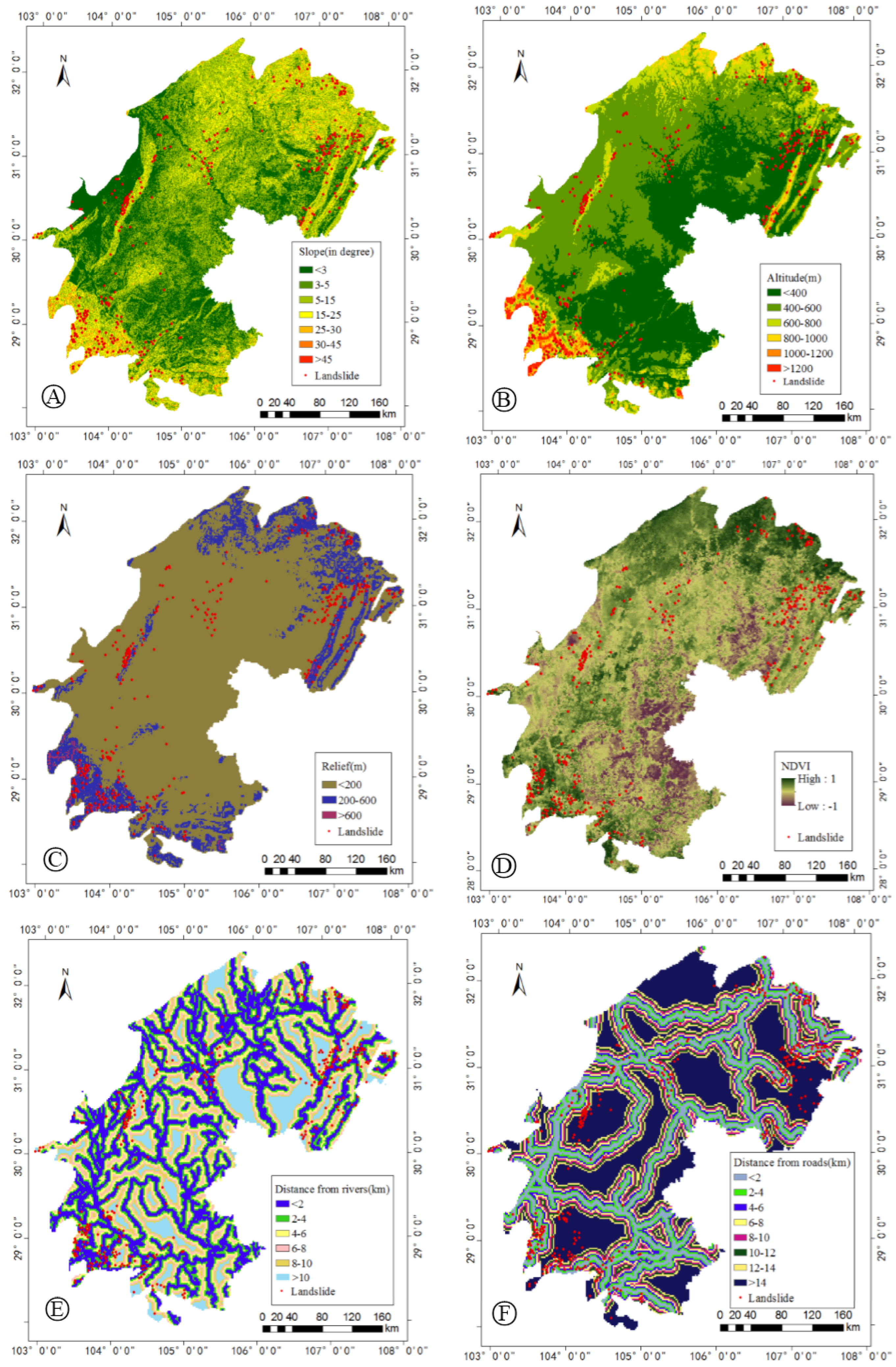
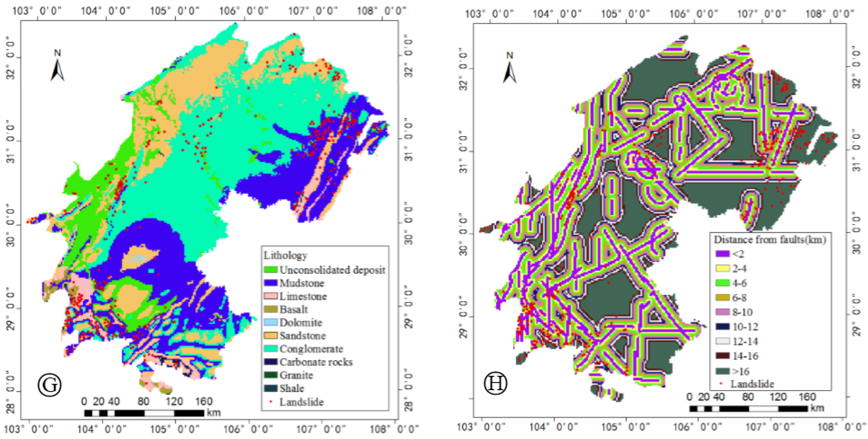
4.1. Influencing Factors of Landslides
4.2. Normalization Processing
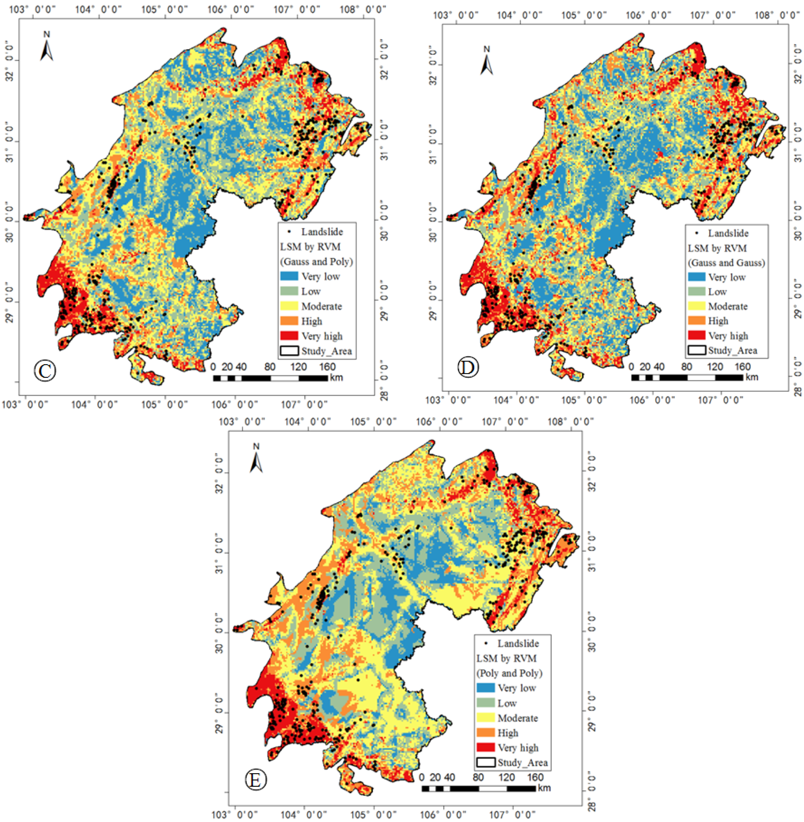
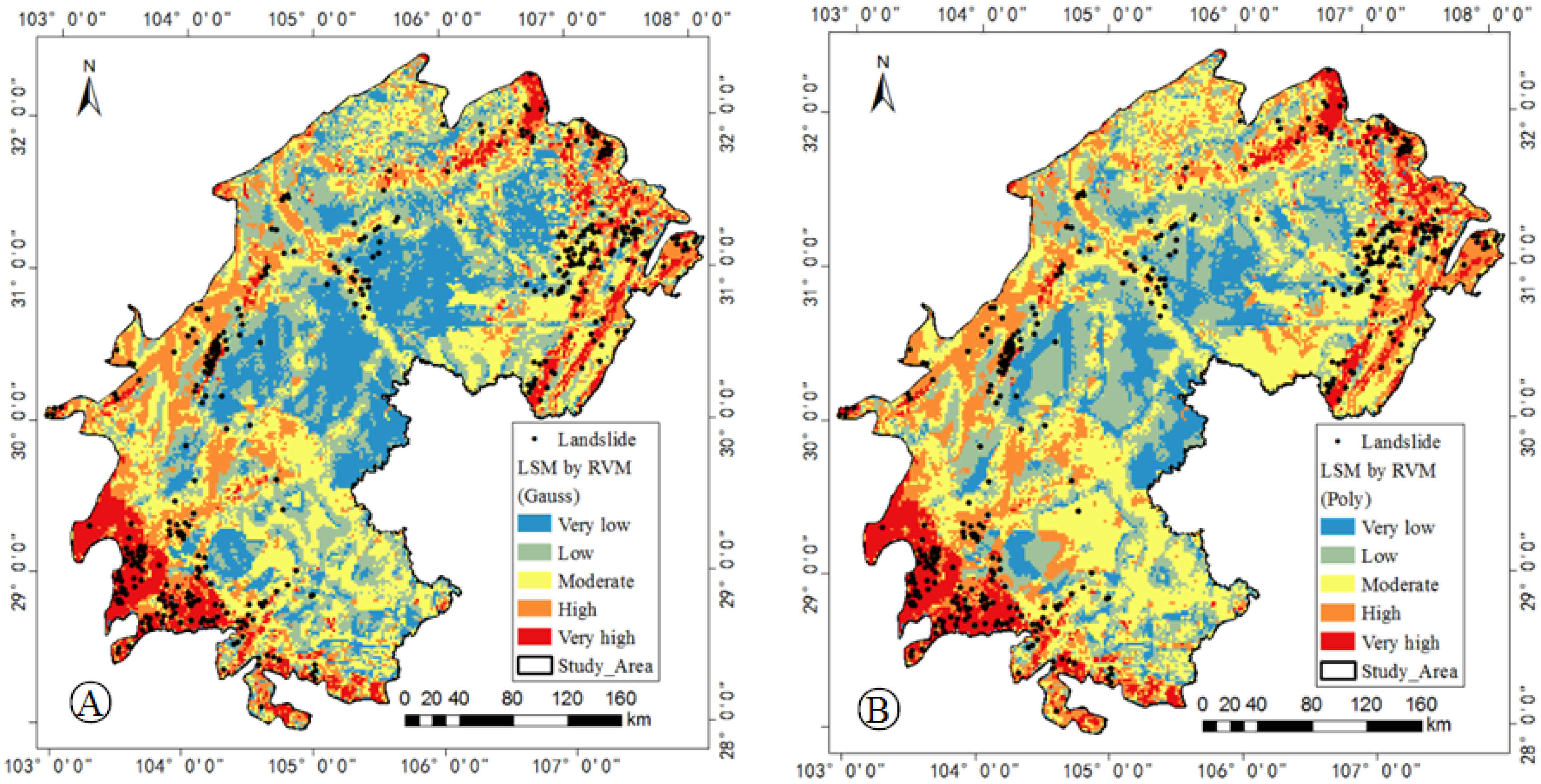
5. Results and Discussion
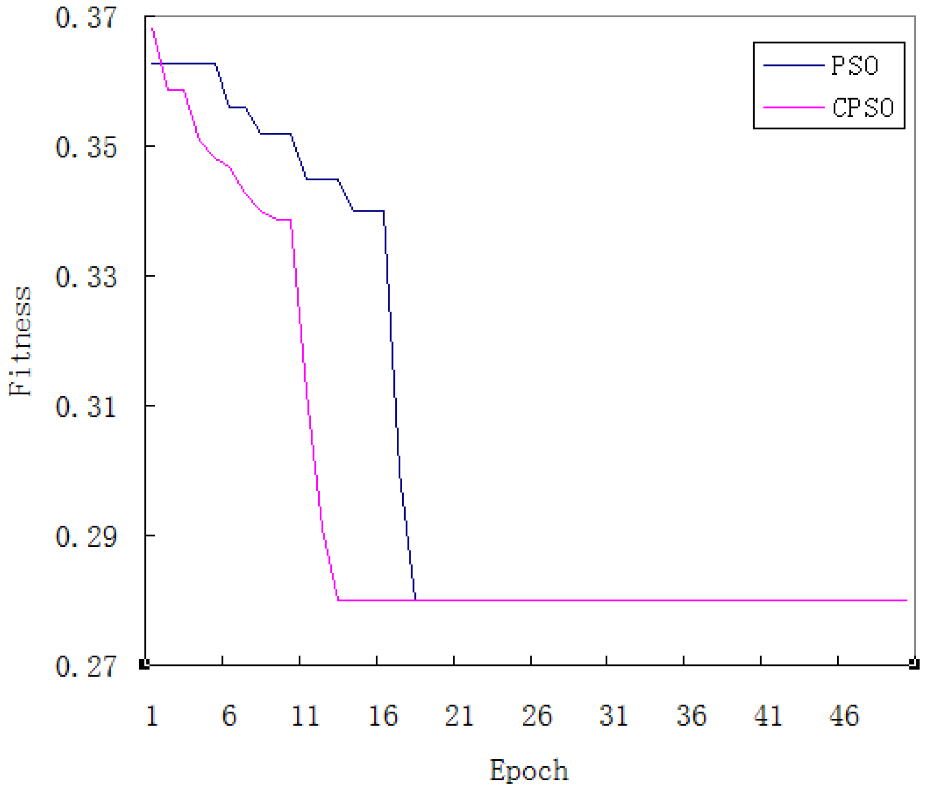
5.1. Model Training
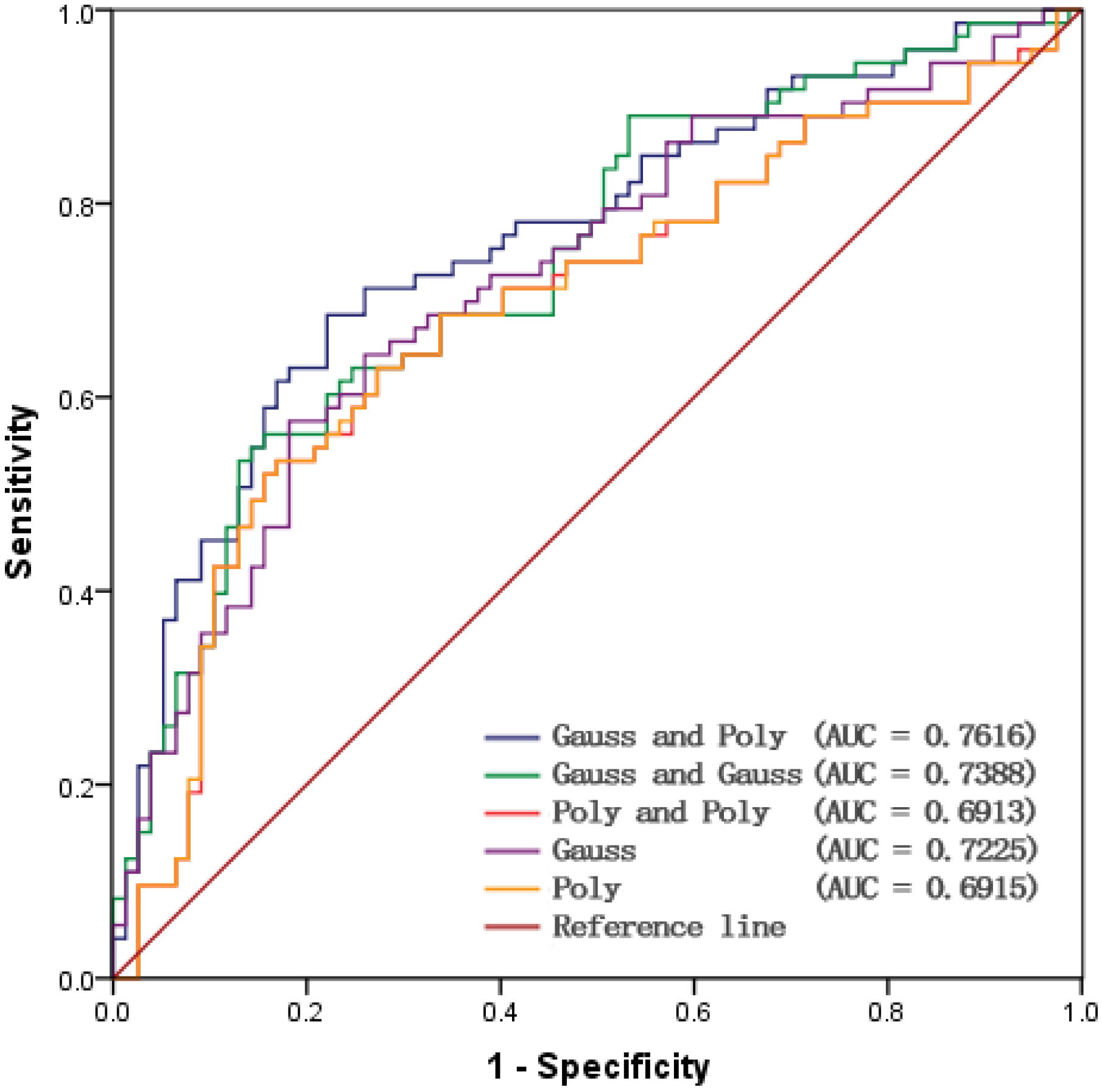
5.2. Receiver Operating Characteristic Curve
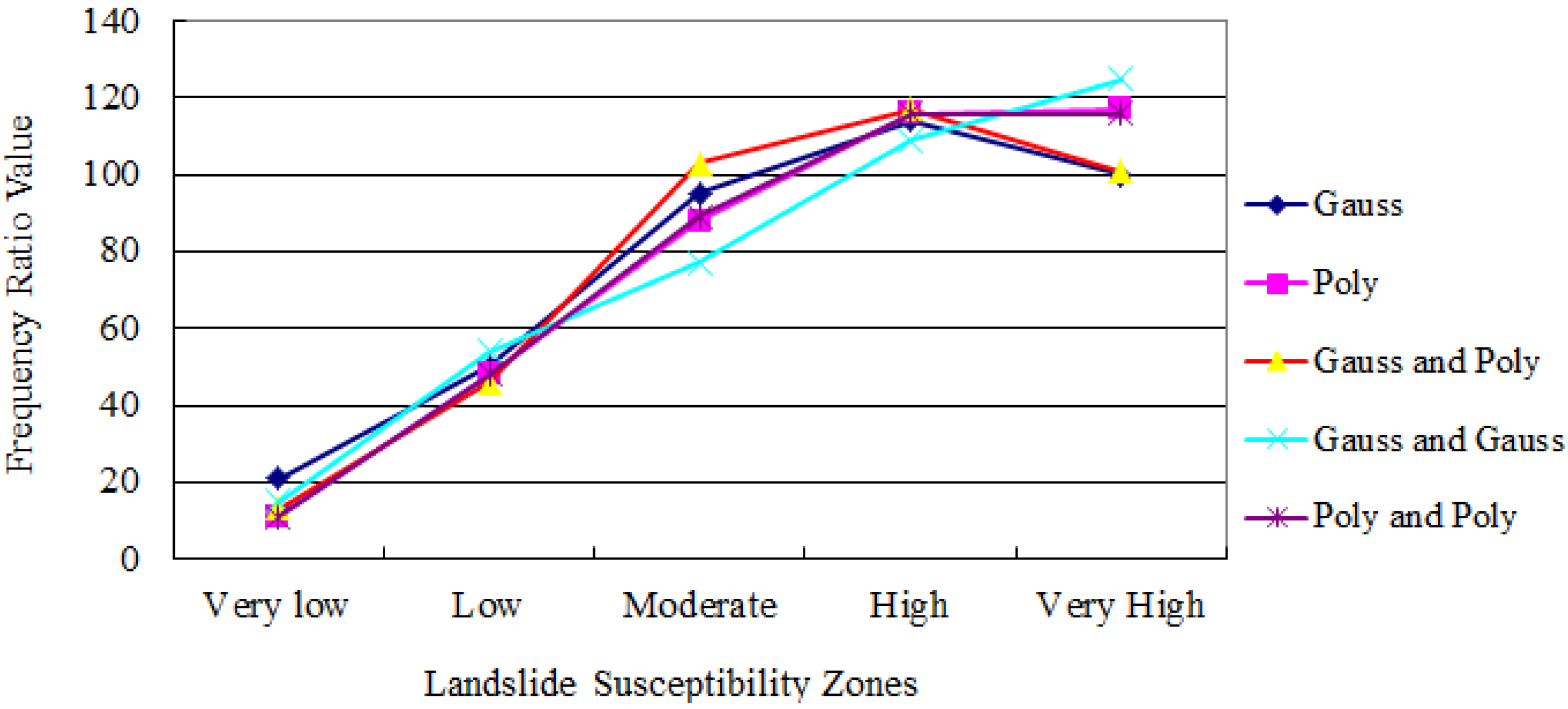
5.3. Landslide Dot Density
6. Conclusions
Acknowledgments
Author Contributions
Conflicts of Interest
References
- Powell, G. Landslide risk management concepts and guidelines. Aust. Geomech. 2000, 35, 49–92. [Google Scholar]
- Chen, X.L.; Ran, H.L.; Qi, S.W. Triggering factors susceptibility of earthquake-induced landslides in 1976 Longling earthquake. Acta Sci. Nat. Univ. Pekinensis 2009, 45, 104–110. (In Chinese) [Google Scholar]
- Pradhan, B. Manifestation of an advanced fuzzy logic model coupled with Geo-information techniques to landslide susceptibility mapping and their comparison with logistic regression modeling. Environ. Ecol. Stat. 2011, 18, 471–493. [Google Scholar] [CrossRef]
- Wu, X.L.; Niu, R.Q.; Ren, F.; Peng, L. Landslide susceptibility mapping using rough sets and back-propagation neural networks in the Three Gorges, China. Environ. Earth Sci. 2013, 70, 1307–1318. [Google Scholar] [CrossRef]
- Ling, P.; Niu, R.Q.; Huang, B.; Wu, X.L.; Zhao, Y.N.; Ye, R.Q. Landslide susceptibility mapping based on rough set theory and support vector machines: A case of the Three Gorges area, China. Geomorphology 2014, 204, 287–301. [Google Scholar]
- Melchiorre, C.; Matteucci, M.; Azzoni, A.; Zanchi, A. Artificial neural networks and cluster analysis in landslide susceptibility zonation. Geomorphology 2008, 94, 379–400. [Google Scholar] [CrossRef]
- Wu, X.L.; Ren, F.; Niu, R.Q. Landslide susceptibility assessment using object mapping units, decision tree, and support vector machine models in the Three Gorges of China. Environ. Earth Sci. 2014, 71, 4725–4738. [Google Scholar] [CrossRef]
- Isik, Y. Comparison of landslide susceptibility mapping methodologies for Koyulhisar, Turkey: Conditional probability, logistic regression, artificial neural networks, and support vector machine. Environ. Earth Sci. 2010, 61, 832–836. [Google Scholar]
- Pourghasemi, H.R.; Jirandeh, A.G.; Pradhan, B.; Chong, X.U.; Gokceoglu, C. Landslide susceptibility mapping using support vector machine and GIS at the Golestan Province, Iran. J. Earth Syst. Sci. 2013, 122, 349–369. [Google Scholar] [CrossRef] [Green Version]
- Tipping, M.E. Sparse bayesian learning and the relevance vector machine. J. Mach. Learn. Res. 2001, 1, 211–244. [Google Scholar]
- Vapnik, V.N. The Nature of Statistical Learning Theory, 2nd ed.; Springer: New York, NY, USA, 2000. [Google Scholar]
- Faul, A.C.; Tipping, M.E. Analysis of sparse bayesian learning. In Proceedings of the Advances in Neural Information Processing Systems 14, Vancouver, BC, Canada, 3–8 December 2001.
- Liu, Z.B.; Shao, J.F.; Xu, W.Y. Comparison on landslide nonlinear displacement analysis and prediction with computational intelligence approaches. Landslides 2014, 11, 889–896. [Google Scholar] [CrossRef]
- Lin, Y.L.; Wang, Z.H.; Xia, K.W.; Li, Z.G. Regional landslide susceptibility assessment based on relevance vector machine. J. Inf. Comput. Sci. 2015, 12, 6893–6903. [Google Scholar] [CrossRef]
- Close, R.; Wilson, J.; Gader, P. A bayesian approach to localized multi-kernel learning using the relevance vector machine. In Proceedings of the International Geoscience and Remote Sensing Symposium (IGARSS), Vancouver, BC, Canada, 24–29 July 2011.
- Gönen, M.; Ethem, A. Multiple kernel learning algorithms. J. Mach. Learn. Res. 2011, 12, 2211–2268. [Google Scholar]
- Mehmet, G.; Ethem, A. Localized algorithms for multiple kernel learning. Pattern Recognit. 2013, 46, 798–807. [Google Scholar]
- Wang, H.Q.; Sun, F.C.; Cai, Y.N. On multiple kernel learning methods. Acta Autom. Sin. 2010, 36, 1037–1050. [Google Scholar] [CrossRef]
- Li, D.X.; Wang, J.; Zhao, X.Q.; Liu, Y.; Wang, D.W. Multiple kernel-based multi-instance learning algorithms for image classification. J. Vis. Commun. Image Represent. 2014, 25, 1112–1117. [Google Scholar] [CrossRef]
- Kennedy, J.; Eberhart, R. Particle swarm optimization. In Proceedings of the IEEE International Conference on Neural Networks, Washington, DC, USA, 27 November–1 December 1995.
- Shi, Y.; Eberhart, R.C. A modified particle swarm optimizer. In Proceedings of the IEEE International Conference on Evolutionary Computation, Anchorage, AK, USA, 4–9 May 1998.
- Liang, X.; Li, W.; Zhang, Y.; Zhou, M. An adaptive particle swarm optimization method based on clustering. Soft Comput. 2015, 19, 431–448. [Google Scholar] [CrossRef]
- Li, J.; Zhang, J.; Jiang, C.; Zhou, M.C. Composite particle swarm optimizer with historical memory for function optimization. IEEE Trans. Cybern. 2015, 45, 2350–2363. [Google Scholar] [CrossRef] [PubMed]
- Li, G.D.; Hu, J.P.; Xia, K.W. Intrusion detection using relevance vector machine based on cloud particle swarm optimization. Control Decis. 2015, 30, 698–702. [Google Scholar]
- Liu, Q.F.; Bo, H.L.; Qin, B.K. Optimization of direct action solenoid valve based on Cloud PSO. Ann. Nucl. Energy 2013, 53, 299–308. [Google Scholar] [CrossRef]
- Duan, Q.; Zhao, J.G.; Ma, Y. Relevance vector machine based on particle swarm optimization of compounding kernels in electricity load forecasting. Electr. Mach. Control 2010, 14, 33–38. (In Chinese) [Google Scholar]
- Fei, S.W.; He, Y.; Ma, X.J.; Miao, Y.B. A hybrid model of RVM and PSO for dissolved gases content forecasting in transformer oil. Recent Pat. Electr. Electr. Eng. 2013, 6, 183–189. [Google Scholar] [CrossRef]
- Fei, S.W.; He, Y. A multiple-kernel relevance vector machine with nonlinear decreasing inertia weight PSO for state prediction of bearing. Shock Vib. 2015, 2015, 1–6. [Google Scholar] [CrossRef]
- Zhang, C.L.; He, Y.G.; Yuan, L.F.; Deng, F.M. A novel approach for analog circuit fault prognostics based on improved RVM. J. Electr. Test. Theory Appl. 2014, 30, 343–356. [Google Scholar] [CrossRef]
- Antoine, S.; Isabel, M.; Van Wesemael, B. Soil organic carbon predictions by airborne imaging spectroscopy: Comparing cross-validation and validation. Soil Sci. Soc. Am. J. 2012, 76, 2174–2183. [Google Scholar]
- Fushik, T. Estimation of prediction error by using K-fold cross-validation. Stat. Comput. 2011, 21, 137–146. [Google Scholar] [CrossRef]
- Milos, M. Comparing the performance of different landslide susceptibility models in ROC space. In Proceedings of the Landslide Science and Practice: Landslide Inventory and Susceptibility and Hazard Zoning, Rome, Italy, 3–9 October 2011.
- Bradley, A.P. Use of the area under the ROC curve in the evaluation of machine learning algorithms. Pattern Recognit. 1997, 30, 1145–1159. [Google Scholar] [CrossRef]
- John, M.; Jha, V.K.; Rawat, G.S. Landslide susceptibility zonation mapping and its validation in part of Garhwal Lesser Himalaya, India, using binary logistic regression analysis and receiver operating characteristic curve method. Landslides 2009, 6, 17–26. [Google Scholar]
- Goetz, J.N.; Brenning, A.; Petschko, H.; Leopold, P. Evaluating machine learning and statistical prediction techniques for landslide susceptibility modeling. Comput. Geosci. 2015, 81, 1–11. [Google Scholar] [CrossRef]
- Fratinni, P.; Crosta, G.; Carrara, A. Techniques for evaluating the performance of landslide susceptibility models. Eng. Geol. 2010, 111, 62–72. [Google Scholar] [CrossRef]
- Yu, S.H. Analyses on spatial-temporal characteristics of mud-rock flow and landslide in Sichuan basin and its meteorological cause. Plateau Meteorol. 2003, 22, 83–89. (In Chinese) [Google Scholar]
- Tang, X.C.; Xie, S.Y. The exploration on the causes of geotectonic to form the regularity of distribution of the mountain calamity landforms surrounding Sichuan Basin. J. Soil Water Conserv. 1994, 8, 76–84. (In Chinese) [Google Scholar]
- Wang, Z.H.; Hu, Z.W.; Liu, C.Q. Susceptibility analysis of disaster-pregnant environmental factors of landslide in the hilly area in Sichuan based on variable dimension fractal theory. Earth Environ. 2013, 41, 680–687. (In Chinese) [Google Scholar]
- Wang, Z.H.; Hu, Z.W.; Zhao, W.J.; Gong, H.L.; Deng, J.X. Susceptibility analysis of precipitation-induced landslide disaster-pregnant environmental factors based on the certainty factor probability model—Taking the hilly area in Sichuan as example. J. Catastrophol. 2014, 29, 109–115. (In Chinese) [Google Scholar]
- Zhang, S.Y. Basis of Geological Disaster Weather Forecast; China Meteorological Press: Beijing, China, 2009. (In Chinese) [Google Scholar]
- Huang, Q. On prevention of landslide in low mountains and hills country in Jiangxi province. J. Jiangxi Norm. Univ. 1992, 2, 161–166. (In Chinese) [Google Scholar]


| Groups | Factors | Subclasses | Area (%) | Factors | Subclasses | Area (%) |
|---|---|---|---|---|---|---|
| Landform | Slope | 0–3° | 20.57 | Altitude | 0–400 m | 37.2 |
| 3–5° | 17.09 | 400–600 m | 45.84 | |||
| 5–15° | 43.01 | 600–800 m | 11.31 | |||
| 15–25° | 14.42 | 800–1000 m | 3.41 | |||
| 25–30° | 2.55 | 1000–1200 m | 1.18 | |||
| 30–45° | 2.13 | >1200 m | 1.06 | |||
| >45° | 0.24 | |||||
| Geological structure | Faults (buffer distance) | 0–2 km | 5.83 | Faults (buffer distance) | 10–12 km | 8.84 |
| 2–4 km | 14.36 | 12–14 km | 7.54 | |||
| 4–6 km | 13.68 | 14–16 km | 6.26 | |||
| 6–8 km | 12.09 | >16 km | 5.04 | |||
| 8–10 km | 10.23 | |||||
| Cutting slope | River network (buffer distance) | 0–2 km | 10.14 | Road network (buffer distance) | 0–2 km | 13.6 |
| 2–4 km | 33.49 | 2–4 km | 11.65 | |||
| 4–6 km | 22.16 | 4–6 km | 10.43 | |||
| 6–8 km | 16.01 | 6–8 km | 9.16 | |||
| 8–10 km | 11.17 | 8–10 km | 8.38 | |||
| >10 km | 7.02 | 10–12 km | 7.48 | |||
| Relief amplitude | 0–200 m | 71.81 | 12–14 km | 6.36 | ||
| 200–600 m | 25.96 | >14 km | 32.93 | |||
| >600 m | 2.23 | |||||
| Geological lithology | Lithology | Unconsolidated deposits | 9.96 | Lithology | Conglomerates | 37.7 |
| Mudstone | 26.78 | Dolomite | 0.54 | |||
| Carbonate rocks | ||||||
| Limestone | 3.35 | Granite | ||||
| Basalt | 0.84 | |||||
| Sandstone | 20.83 | Shale | ||||
| Vegetation | NDVI | −1–1 |
| Model (Kernel Type) | Weight | Width 1 | Width 2 | Error Rate (ER) |
|---|---|---|---|---|
| Gauss | 1 | 0.313 | ||
| Poly | 0.8443 | 0.333 | ||
| Gauss and Poly | 0.6831 | 0.6138 | 2 | 0.28 |
| Gauss and Gauss | 0.2366 | 0.3396 | 1 | 0.333 |
| Poly and Poly | 0.114 | 0.6 | 0.8844 | 0.333 |
| Landslide Susceptibility Zone | LDD (/100 km2) | ||||
|---|---|---|---|---|---|
| Gauss | Poly | Gauss and Poly | Poly and Poly | Gauss and Gauss | |
| Very low | 0.36 | 0.33 | 0.24 | 0.33 | 0.24 |
| Low | 0.71 | 0.65 | 0.58 | 0.65 | 0.71 |
| Moderate | 1.24 | 0.98 | 1.36 | 0.99 | 1.22 |
| High | 2.3 | 2.03 | 2.52 | 2.04 | 2.35 |
| Very high | 4.1 | 4.47 | 4.19 | 4.42 | 3.94 |
| Sum of low and very low | 1.7 | 0.98 | 0.82 | 0.98 | 0.95 |
| Sum of high and very high | 6.4 | 6.5 | 6.71 | 6.46 | 6.29 |
© 2016 by the authors; licensee MDPI, Basel, Switzerland. This article is an open access article distributed under the terms and conditions of the Creative Commons Attribution (CC-BY) license (http://creativecommons.org/licenses/by/4.0/).
Share and Cite
Lin, Y.; Xia, K.; Jiang, X.; Bai, J.; Wu, P. Landslide Susceptibility Mapping Based on Particle Swarm Optimization of Multiple Kernel Relevance Vector Machines: Case of a Low Hill Area in Sichuan Province, China. ISPRS Int. J. Geo-Inf. 2016, 5, 191. https://0-doi-org.brum.beds.ac.uk/10.3390/ijgi5100191
Lin Y, Xia K, Jiang X, Bai J, Wu P. Landslide Susceptibility Mapping Based on Particle Swarm Optimization of Multiple Kernel Relevance Vector Machines: Case of a Low Hill Area in Sichuan Province, China. ISPRS International Journal of Geo-Information. 2016; 5(10):191. https://0-doi-org.brum.beds.ac.uk/10.3390/ijgi5100191
Chicago/Turabian StyleLin, Yongliang, Kewen Xia, Xiaoqing Jiang, Jianchuan Bai, and Panpan Wu. 2016. "Landslide Susceptibility Mapping Based on Particle Swarm Optimization of Multiple Kernel Relevance Vector Machines: Case of a Low Hill Area in Sichuan Province, China" ISPRS International Journal of Geo-Information 5, no. 10: 191. https://0-doi-org.brum.beds.ac.uk/10.3390/ijgi5100191