A Framework for Discovering Evolving Domain Related Spatio-Temporal Patterns in Twitter

Abstract

In massive Twitter datasets, tweets deriving from different domains, e.g., civil unrest, can be extracted to constitute spatio-temporal Twitter events for spatio-temporal distribution pattern detection. Existing algorithms generally employ scan statistics to detect spatio-temporal hotspots from Twitter events and do not consider the spatio-temporal evolving process of Twitter events. In this paper, a framework is proposed to discover evolving domain related spatio-temporal patterns from Twitter data. Given a target domain, a dynamic query expansion is employed to extract related tweets to form spatio-temporal Twitter events. The new spatial clustering approach proposed here is based on the use of multi-level constrained Delaunay triangulation to capture the spatial distribution patterns of Twitter events. An additional spatio-temporal clustering process is then performed to reveal spatio-temporal clusters and outliers that are evolving into spatial distribution patterns. Extensive experiments on Twitter datasets related to an outbreak of civil unrest in Mexico demonstrate the effectiveness and practicability of the new method. The proposed method will be helpful to accurately predict the spatio-temporal evolution process of Twitter events, which belongs to a deeper geographical analysis of spatio-temporal Big Data.

1. Introduction

Spatio-temporal Big Data has the characteristics of volume, variety, velocity, veracity and value. And nowadays the knowledge discovery from spatio-temporal Big Data is mainly focused on summarization, obfuscated outliers, rare associations, and obfuscated process prediction, which are expansions of traditional spatio-temporal data mining. In location-based social networks, Twitter has attracted the largest number of users since its launch in 2006 [1]. As mobile phones become more intelligent and wireless network coverage expands, anyone with a mobile phone can send tweets almost anywhere, anytime. As a result, Twitter has experienced an explosive growth in its user base [2]. Nowadays most intelligent mobile phones are GPS-enabled, so geographical location information is often included as an additional tag in tweets. Combined with the time annotation, this type of spatio-temporal information can be embedded in tweets to describe where and when the tweets are broadcast. So the Twitter data has become a kind of spatio-temporal Big Data. Due to the high degree of freedom and openness of Twitter, massive amounts of useless information that is unrelated to significant events is broadcast that simply reports common interactions among friends. Moreover, Twitter can be considered as a large black box that contains numerous topics reflecting various events from different domains, e.g., disasters [3], crimes [4], traffic [5], and epidemics [6]. Ways to extract hidden, unknown and significant events from the huge mass of Twitter data has thus become a research hotspot in computer science [7,8], human science [9,10] and GIS [11,12,13,14] in recent years. The research approaches applied can be roughly classified into three categories depending on which of the above three fields is the focus: (1) scholars in computer science consider tweets as textual information that changes over time, so topics related to different domains can be extracted by text classification methods such as Latent Dirichlet Allocation (LDA) and clustering; (2) in human science, scholars usually treat Twitter as a tool to record human behaviors; for example moving behaviors can be reflected by the changes in number of Twitter users coming into and going out of a certain region; and (3) researchers in GIS commonly extract domain related events to identify spatio-temporal outliers or hotspots. The research reported here utilized the third of these approaches to spatio-temporal pattern detection from Twitter.

In a spatio-temporal event dataset, each entity represents an event that occurred at the location and time tagged [15]. Further, spatio-temporal Twitter events are defined as a series of point entities with geo-location and time information embedded in domain related tweets. Taking Figure 1 as an example, this depicts the spatio-temporal Twitter events related to ‘civil unrest’ for the month of July, 2012 throughout Mexico. Unlike previous research in this area, the spatio-temporal approach proposed here focuses specifically on the evolution of domain related spatio-temporal patterns in Twitter. The major contributions of this study are as follows:

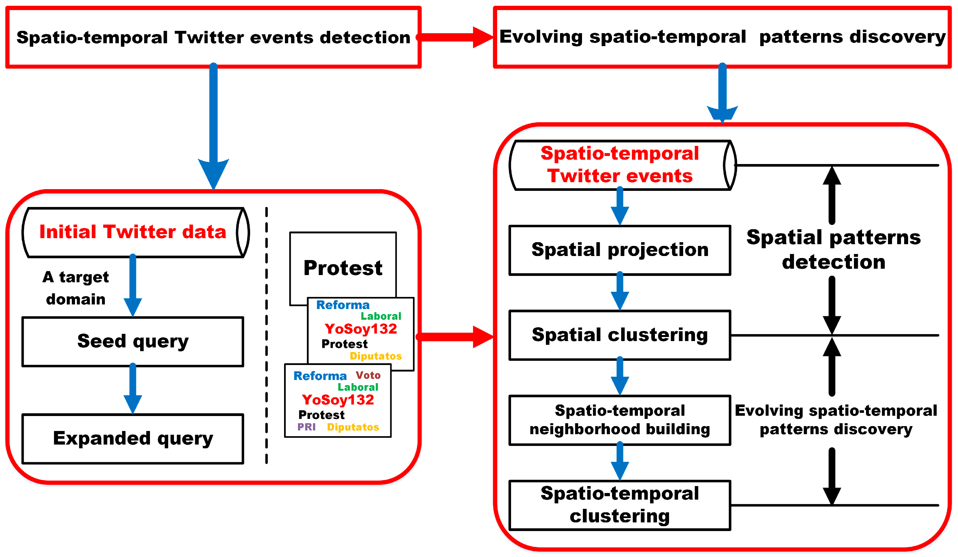
• Development of a mining framework: a unified framework is proposed to discover evolving domain-related spatio-temporal patterns in Twitter. Prior knowledge is not required in the new framework.
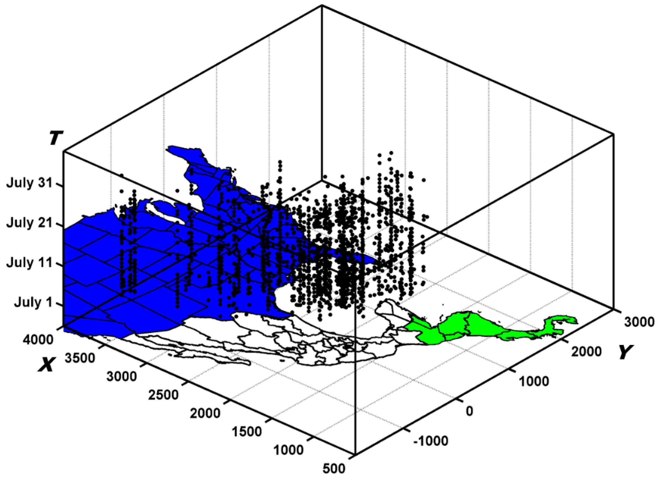
• Extraction of domain related Twitter events by dynamic query expansion: For the target domain, related tweets can be obtained using a dynamic query expansion strategy. These tweets tagged with geo-location and time information constitute spatio-temporal Twitter events.
• Discovery of evolving spatio-temporal patterns from Twitter events: For the extracted domain related spatio-temporal Twitter events, spatial clusters and outliers are detected by spatial clustering, after which the spatio-temporal patterns are discovered by spatio-temporal clustering as they evolve.
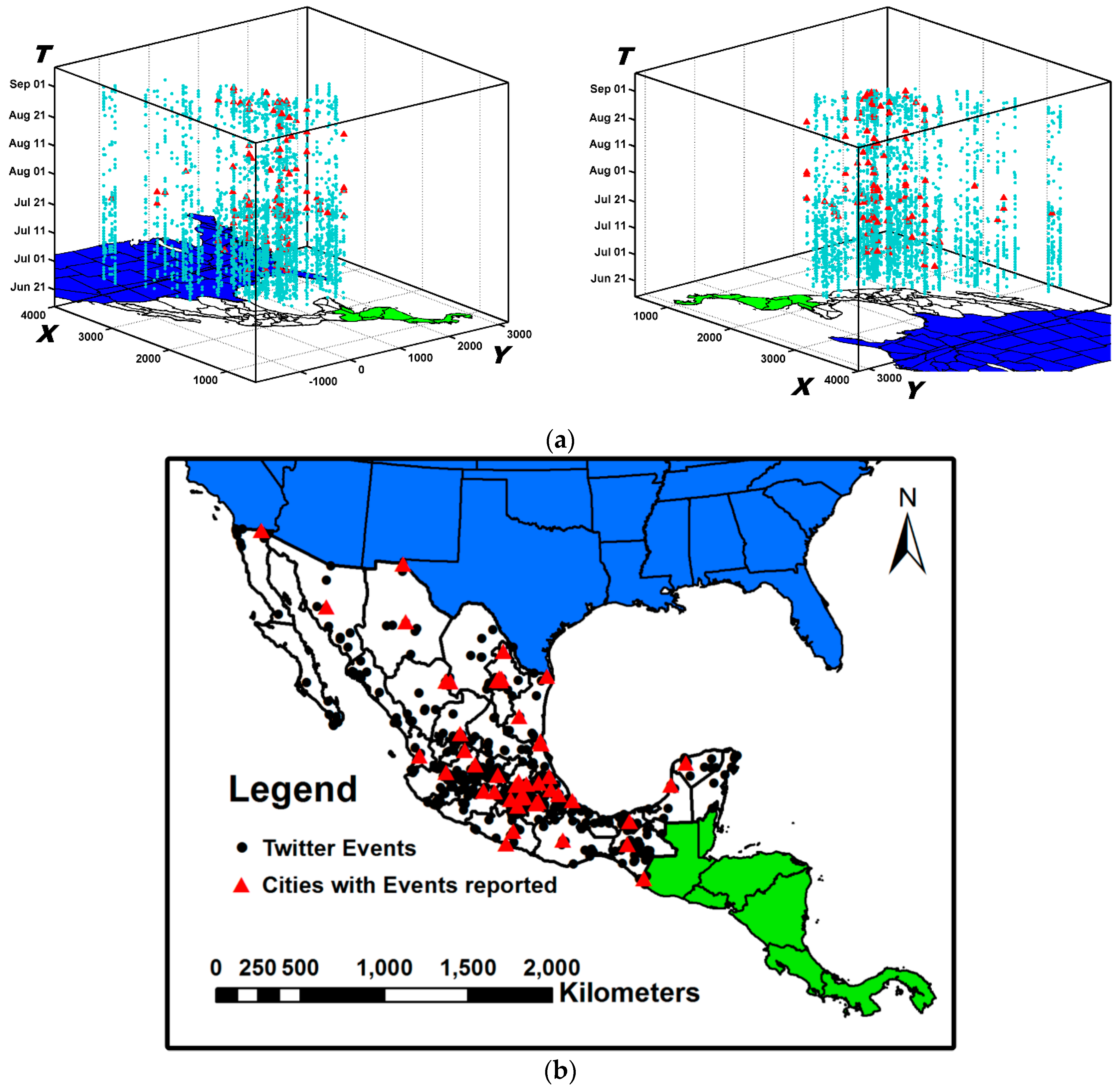
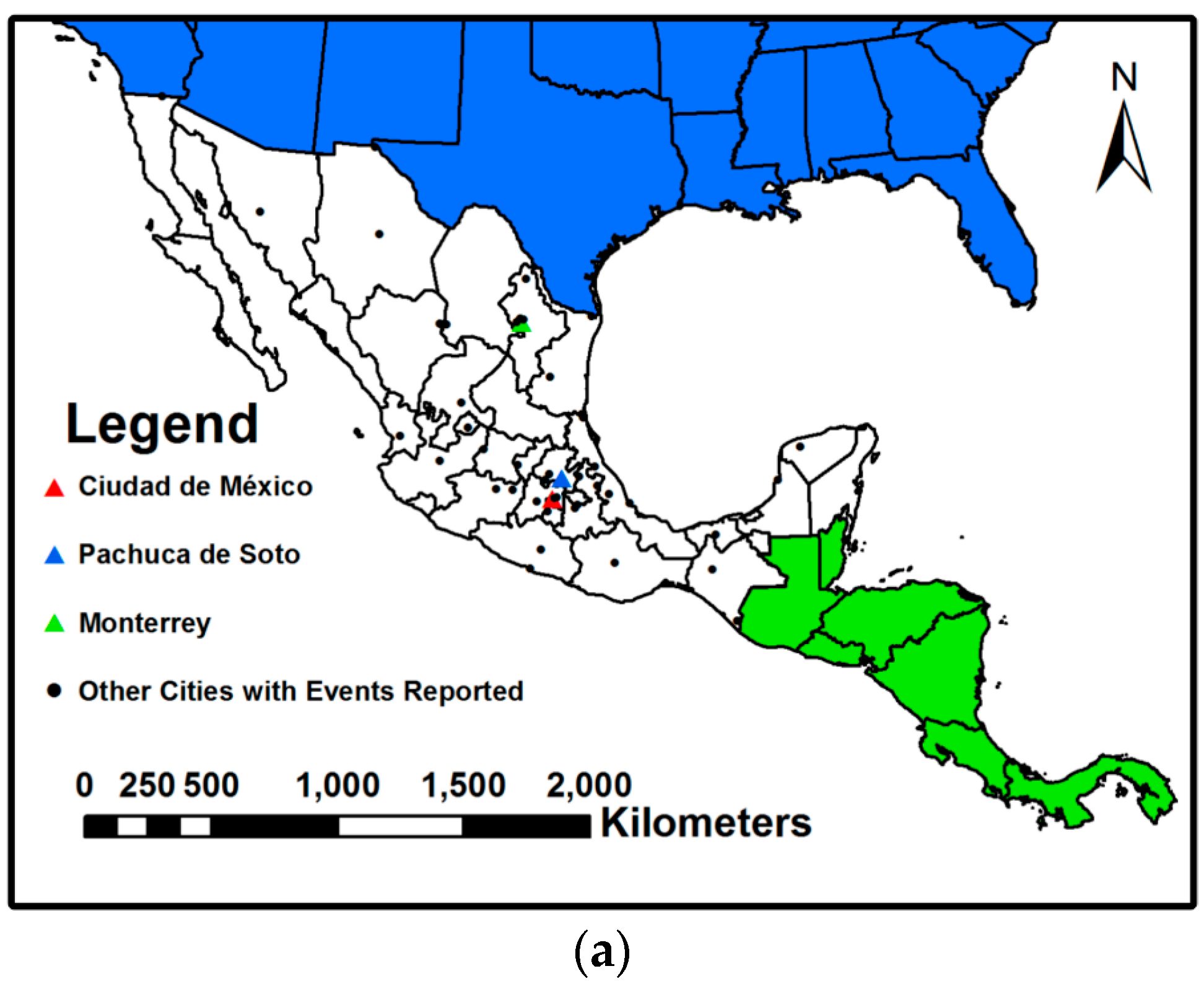
• Experimental evaluation using real Twitter data: The proposed framework was extensively tested for spatio-temporal Twitter events related to ‘civil unrest’ in Mexico. The advantages and effectiveness of the new method are demonstrated by comparing the results with alternative methods and baseline data.

The rest of this paper is organized as follows. Section 2 reviews the related work and Section 3 explains our motivation and research strategy. Section 4 describes the model used to extract the domain related Twitter events, after which the approach used to discover the spatio-temporal patterns in the Twitter events as they evolved is presented in Section 5. Section 6 reports on the extensive experiments on real world Twitter data and their analysis, and the paper concludes by summarizing the study’s important findings in Section 7.

2. Related work

2.1. Twitter Event Extraction

Existing Twitter event extraction methods mainly derive from machine learning, with approaches such as LDA (Latent Dirichlet Allocation), SVM (Support Vector Machine), and HMM (Hidden Markov Models). LDA is an unsupervised learning algorithm that was originally developed to classify general texts [16] but has more recently been employed to classify Twitter data into different topics [7,8]. SVM is a supervised learning algorithm for classification. Given a target domain, it begins by requiring users to label sections of domain related tweets as samples, after which these training samples are used to extract related tweets [17]. Chakrabarti and Punera (2011) [18] took a different approach, employing a modified HMM model to learn the characteristic of sample tweets and then extract related tweets.

2.2. Cluster, Outlier and Hotspot Detection

In the field of spatio-temporal data mining, spatio-temporal clustering [15,19], outlier detection [20,21] and hotspot detection [22] are all key research techniques. As both geo-location and time information are often embedded in tweets, this facilitating spatio-temporal data mining in Twitter data. Research in this area can be classified into two types: (1) spatio-temporal distribution pattern detection from initial Twitter data; and (2) spatio-temporal distribution pattern detection from domain related Twitter events.

Spatio-temporal distribution pattern detection from initial Twitter data. Here, Twitter data is directly utilized to detect latent spatio-temporal clusters, outliers or hotspots without extracting topics, then deeper analysis is performed on any patterns detected to verify whether a special event has occurred. For example, Lee et al. (2011) [10] divided the whole research region into sub-regions based on the spatial distribution of tweets by clustering. For each sub-region, the time stamps with unusually large number of tweets were then detected by boxplot. Cheng and Wicks (2014) [12] detected spatio-temporal hotspots using space-time scan statistics from Twitter. Different topics were extracted by LDA for each spatio-temporal hotspot and the ratio of topics was used to determine whether the spatio-temporal hotspot described a specific event.

Spatio-temporal distribution pattern detection from domain related Twitter events. In this type of approach, a target domain is usually specified and then spatio-temporal pattern mining performed on domain related tweets. For example, Chae et al. (2012) [11] employed LDA to extract groups of topics related to different domains. For each domain, a time series can be obtained by recording the number of tweets with domain related topics as time progresses. For each time series, after removing any seasonal trends those time stamps recording unusually large numbers of tweets were identified as abnormal events using Z-core. In a previous study, we proposed a dynamic query expansion to extract domain related tweets from Twitter [13]. The extracted tweets constituted a group of spatial events for a given period of time and a local modularity spatial scan was developed to detect spatial hotspots. Bakillah et al. (2014) [14] built social graphs in Twitter based on various interaction modes and enhanced fast-greedy optimization of modularity was employed to extract different thematic communities. For disjoint time periods, spatial clusters were detected by VDBSCAN [23] for each thematic community from a spatial point of view.

In summary, most previous work in this area has focused on detecting fixed spatio-temporal distribution patterns from Twitter. However, there is also an evolving relationship between the spatio-temporal development of a Twitter event and its final spatial distribution. In this paper, we propose a new framework that combines dynamic query expansion with a spatio-temporal mining approach to discover newly evolving domain related spatio-temporal patterns from Twitter.

3. Motivation and Proposed Strategy

3.1. Motivation

Existing domain related tweet extraction methods mostly fail to consider the hidden relationships among tweets. For example, if an earthquake occurs at place ‘A’ then any tweets containing phrases such as ‘A, damage, collapsed buildings’, even if they do not specifically say ‘earthquake’, are also likely to be related to the earthquake. Therefore, it is necessary to analyze the hidden relationships in Twitter data if we are to adequately extract domain related tweets.

Further, existing research on mining spatio-temporal patterns from Twitter events focuses primarily on detecting outliers or hotspots directly from the distribution of the tweets; over a given time period these spatio-temporal Twitter events can evolve into certain spatial distribution patterns, e.g., spatial clusters or outliers. However, to the best of our knowledge there have not been studies seeking to discover the spatio-temporal evolution process for each spatial pattern. For example, a group of tweets representing a spatio-temporal event dataset with 10 time stamps is simulated in Figure 2. Figure 2a gives the spatio-temporal distribution while Figure 2b shows the spatial projection of all events. Figure 2c is the spatial projection at each time stamp. The spatial distribution patterns formed by all spatio-temporal events for this time period are hidden in Figure 2b, which contains four types of patterns: spatial clusters, global spatial outliers, local spatial outliers and inner spatial outliers. In Figure 2c, events at each stamp are differently labeled based on the patterns in Figure 2b. The evolving process by which each of the three distinct spatial patterns develops is as follows: (1) a dense cluster derives from its center at T = 1 and extends until the whole cluster is formed at T = 4, after which this cluster gradually diminishes from its center and disappears at T = 8; (2) For a sparse cluster, events appear to arise randomly in its upper section from T = 1 to 4 and only after T = 5 does the lower part of this cluster gradually come into being. At T = 7, some events in the upper section begin to appear again; and (3) Global outliers are present at all times, but the local outliers appear only between T = 3 and 7. The inner spatial outliers are formed gradually from the center from T = 4 to 6 and then do not change.

By integrating the spatial distribution of Twitter events at different time stamps shown in Figure 2c, in the research we are aiming to discover those spatio-temporal clusters or outliers, i.e., evolving spatio-temporal patterns, which will evolve into the final spatial distribution patterns shown in Figure 2b.

3.2. A New Strategy for Discovering Evolving Domain Related Spatio-Temporal Patterns in Twitter

To discover and visualize the spatio-temporal patterns evolving in the Twitter data for a given domain, a framework is proposed here that is based on a dynamic query expansion and spatio-temporal pattern mining approach, as shown in Figure 3. There are two main parts in our proposed framework, described in turn below.

Detection of domain related Twitter events. In this part, a model for dynamic query expansion is built to adequately extract domain related Twitter events that consists of: (1) the seed query, where some seeds that directly match the domain are queried; (2) the expanded query, which extracts those tweets related to the domain by considering the relationships hidden in the Twitter data; and (3) the spatio-temporal Twitter event extraction, where the domain related tweets with spatio-temporal information constitute the spatio-temporal Twitter events.

Discovery of evolving spatio-temporal patterns. In this part, a spatio-temporal clustering approach is proposed that consists of: (1) spatial projection, where spatio-temporal Twitter events are spatially projected to obtain the spatial distribution; (2) spatial clustering based on multi-constrained Delaunay triangulation is developed to detect various types of spatial distribution patterns; (3) spatio-temporal neighborhood building, which considers both spatial proximity and time consecutiveness to create spatio-temporal neighborhoods for each Twitter event; and (4) spatio-temporal clustering is performed based on these spatio-temporal neighborhoods to discover any spatio-temporal patterns as they evolve.

4. Domain Related Twitter Event Detection

In this section, a model for the dynamic query expansion is built that is capable of extracting domain related spatio-temporal Twitter events. In Section 4.1, we provide definitions for the terms ‘Twitter information graph’, ‘seed query’, ‘expanded query’ and ‘weight measurement’. Section 4.2 moves on to consider the process of dynamic query expansion, after which spatio-temporal Twitter events are defined in Section 4.3.

4.1. Basic Definitions

Twitter information graph: Given an initial set of Twitter data, an information graph G = (V, E, W, ST) can be obtained. Here, V denotes the nodes in G, which consists of tweets and features (e.g., users, terms, hashtags). E denotes the undirected edges connecting related nodes in G. For example, if a feature exists in some tweets then this feature is connected with these tweets. For each node in G, a weight is assigned and all the weights constitute W. For a given domain, the weights of all the nodes reflect the relevance to this domain. Finally, ST gives the geo-location (e.g., longitude and latitude) and time information embedded in each tweet.

By considering the multiple relationships among tweets and features, those tweets related to a given domain can be extracted by a kind of dynamic query expansion. Two parts, the seed query and the expanded query, are included and these can be described as follows:

Seed query: Given a target domain, the seed query extracts those key words in V that are consistent with the domain semantically. For example, if the given domain is ‘civil unrest’ then the queried seeds can be {(‘protest’), (‘march’)}.

Expanded query: Here the seeds are those nodes that are directly related to the given domain. However, in most situations more related nodes can be queried further based on the seeds. For example, assume the seeds {(‘protest’), (‘march)} are obtained. As {(‘YoSoy132’), (‘Zocal’)} frequently appear in the same tweet with the seeds, for example as: ‘A mega march against the imposition of PRI: YoSoy132 protestors arrived at El Zocalo.’, then {(‘YoSoy132’), (‘Zocal’)} can become key words in an expanded query. The expanded query can then extract those key words in V that are related to the seeds by some hidden relationships.

Weight measurement: Among all the tweets and features in V, there are two main types of relationships, i.e., features ↔ tweets and tweets ↔ tweets. If a feature exists in those tweets with high weights for the domain then this feature will also have a high weight and vice versa. If a tweet replies to another tweet with a high weight then it will also receive a high weight. Thus, the weights of features are mainly affected by the related tweets, while the weights of tweets are determined by both the related features and other tweets with which they have replying relationships. These weights can be described as:

$$W(F)=ID{F}_F•E_{F\leftrightarrow T}•W(T)$$

(1)

$$W(T)={\omega }_1•E_{T\leftrightarrow F}•W(F)+{\omega }_2•E_{T\leftrightarrow T}•W(T)$$

(2)

Here, W(F) and W(T) denote the weights of features and tweets, respectively. E_F↔T denotes a matrix describing the relationship between features and tweets. If a feature belongs to a tweet, the corresponding value in the matrix is equal to 1 and otherwise it is equal to 0. E_T↔F is the transpose of E_F↔T. Similarly, E_T↔T describes the relationship between tweets and other tweets. If a tweet replies to another tweet, the corresponding value in E_T↔T is equal to 1 and otherwise it is equal to 0. IDF_F is the inverse document frequency matrix for the features [24]. ω₁ and ω₂ denote the degree of influence from features and other tweets, respectively, on the analyzed tweet.

4.2. Dynamic Query Expansion

Based on these basic definitions, a dynamic query expansion can be described in the following:

Step I Initialization of domain related nodes: Given a target domain, the seed query proceeds to extract key words. In the tweet set T, the tweets matching these key words consist of the initial domain related tweets T⁽⁰⁾. Those features connected with T⁽⁰⁾ constitute the initial domain features F⁽⁰⁾. The weights of all the tweets in T⁽⁰⁾ are equal to 1 while the weights of other tweets, i.e., those tweets in T − T⁽⁰⁾, are equal to 0.

Step II Expanded query by iteration: For the k^th (k ≥ 2) iteration of the expanded query, the weights of the features in F^(k) and tweets in T^(k) are initially calculated as:

$$W[F^{(k)}]=ID{F}_F•E_{F\leftrightarrow T}•W[T^{(k-1)}]$$

(3)

$$W[T^{(k)}]={\omega }_1•E_{T\leftrightarrow F}•W[F^{(k)}]+{\omega }_2•E_{T\leftrightarrow T}•W[T^{(k-1)}]$$

(4)

Then, for tweets in T^(k) and T − T^(k), if the maximal weigh in T − T^(k) is larger than the minimal weight in T^(k) then the two corresponding tweets will be swapped. This process of swapping will continue until max {W[T − T^(k)]} ≤ min {W[T^(k)]}.

Step III Generation of domain related tweets: For the k^th (k ≥ 2) iteration of the expanded query, after the updating of weights for features in F^(k) and tweets in T^(k), once max {W[T − T^(k)]} ≤ min {W[T^(k)]} is satisfied then the process of the expanded query is terminated. For the final set of domain related features F^(k), all features having at least one edge with the tweets in F^(k) are considered to be highly relevant to the target domain. All tweets containing these domain related features are thus considered to be domain related tweets in T.

The time complexity mainly derives from the dynamic query expansion and is approximately O{n_i[n_F*n_TF + n_T*(n_TF + n_TT)]}, where n_i is the number of iterations performed, n_F and n_T are the number of features and tweets, respectively, n_TF is the number of connections between tweets and a feature, and n_TT is the number of connections between two different tweets. Note that n_TF << n_F and n_TT << n_T.

4.3. Spatio-Temporal Twitter Events

Combining the geo-location and time information embedded in the tweets, the domain related spatio-temporal Twitter events can be defined as:

Spatio-temporal Twitter events: Given a set of extracted domain related tweets, each tweet, along with its geo-location and time information, is considered to be a spatio-temporal Twitter event stte_i, stte_i = (x_i, y_i, t_i), and all spatio-temporal Twitter events constitute a set STTE = {stte₁, stte₂, …, stte_N}.

Spatial Twitter events: Given STTE, the corresponding spatial Twitter events are the spatial distribution of STTE after spatial projection. Taking the simulated dataset in Figure 2 as an example, assume Figure 2a gives the spatio-temporal Twitter events for a target domain. Then Figure 2b shows the corresponding spatial Twitter events. The spatial Twitter events are composed of n spatial points, denoted as STE = {ste₁, ste₂, …, ste_n}. Each spatial Twitter event ste_i includes geo-location information, i.e., ste_i = (x_i, y_i)

5. Evolving Spatio-Temporal Patterns Discovery

This section describes two steps that are performed on the STTE: (1) Spatial distribution pattern detection; and (2) the discovery of evolving spatio-temporal patterns. Section 5.1 examines the approach used for the spatial distribution pattern detection, while the process of discovering spatio-temporal patterns as they evolve is described in Section 5.2. Finally, the algorithms are described in Section 5.3.

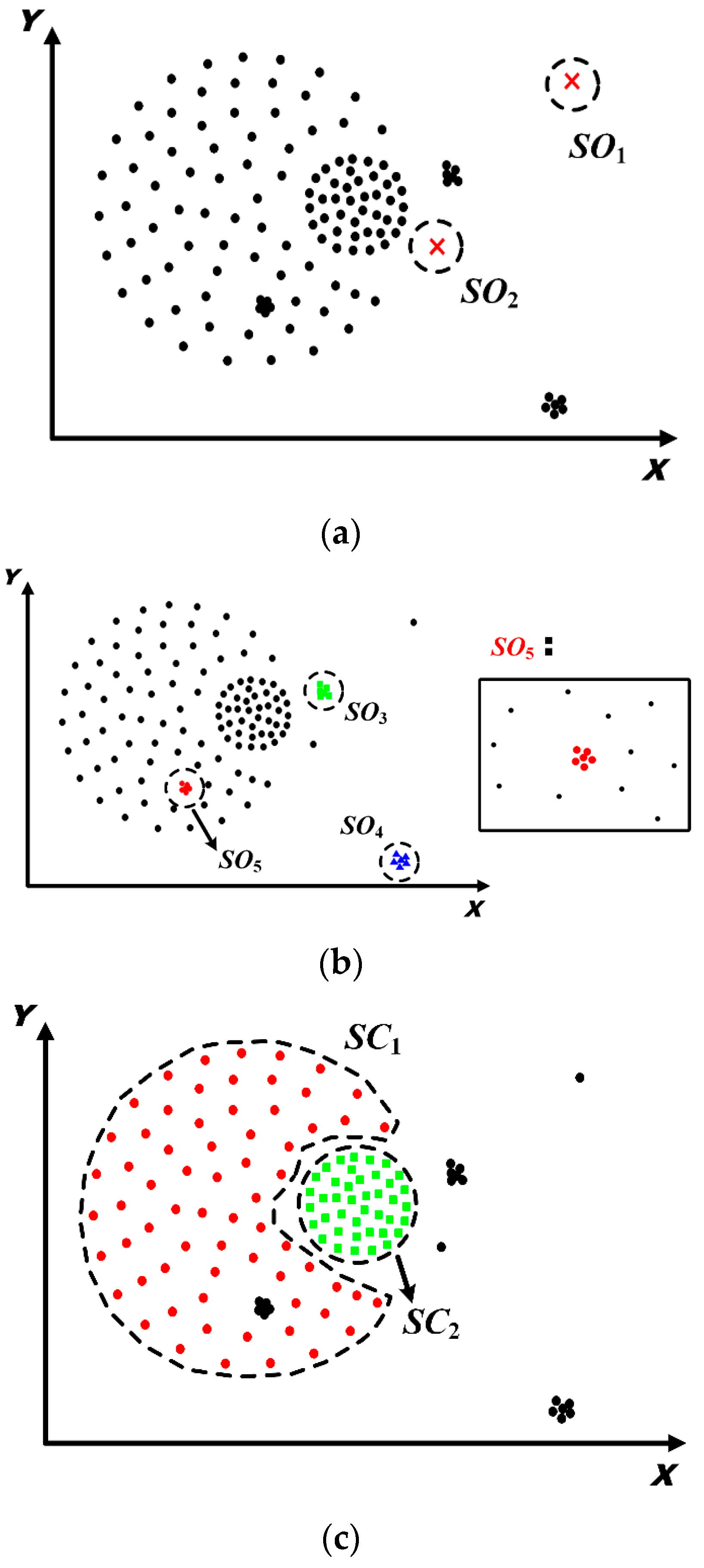
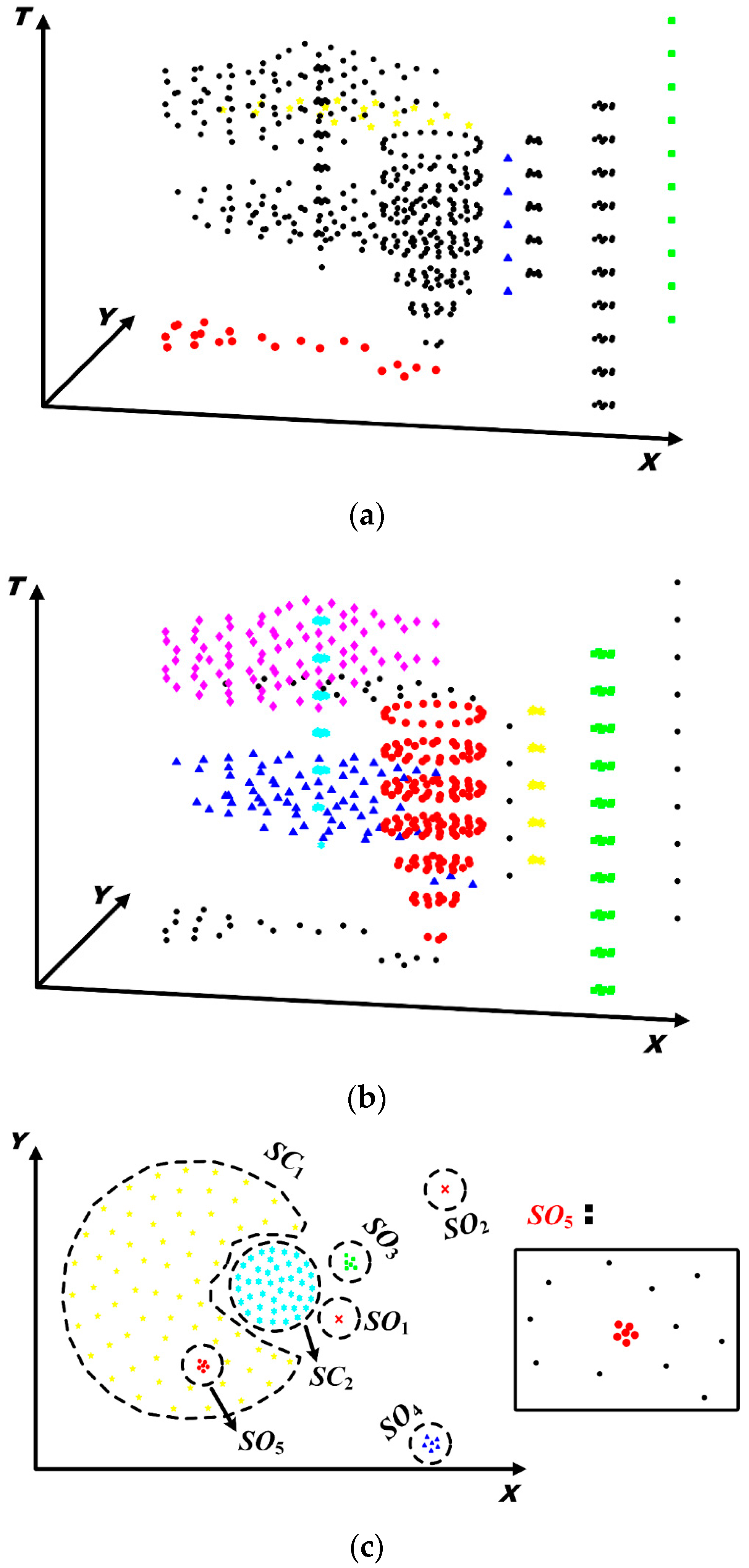
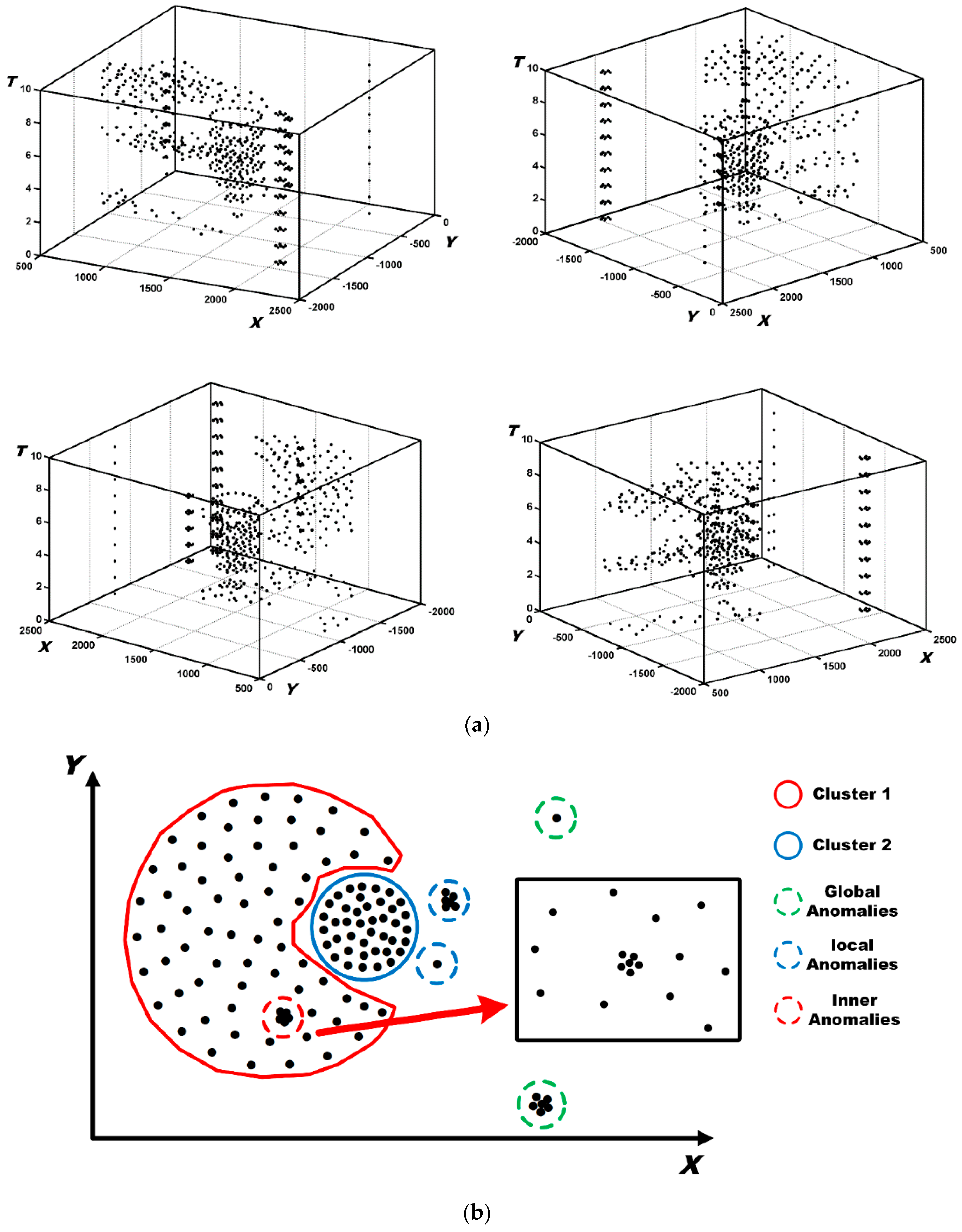
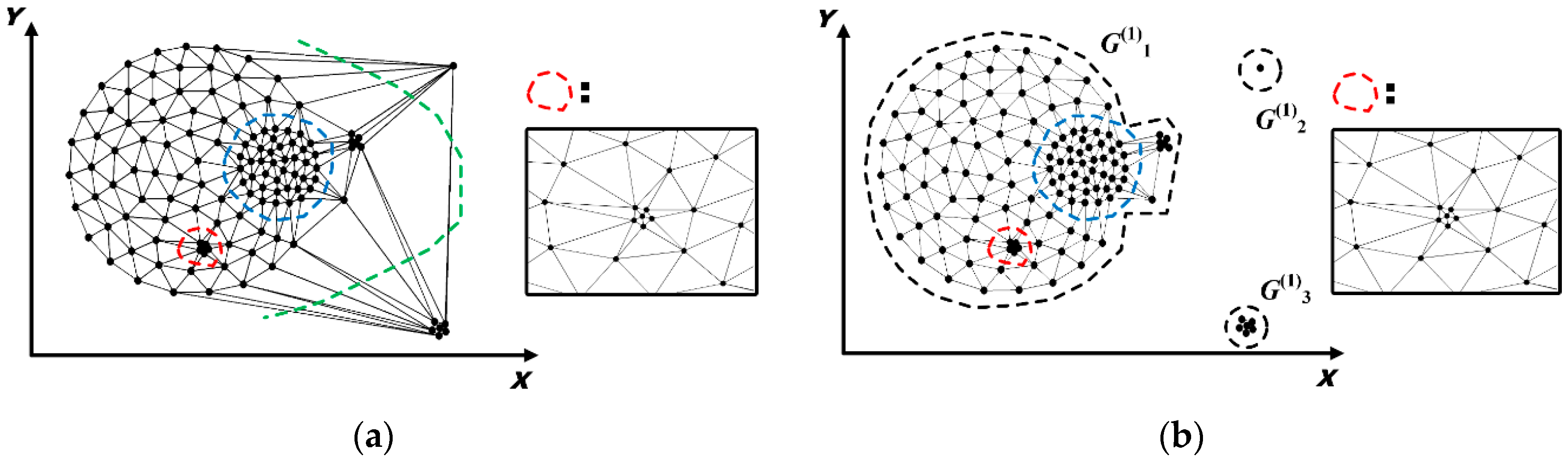
5.1. Spatial Distribution Patterns Detection

In order to detect spatial distribution patterns from spatial point events, a number of spatial clustering [25,26] and spatial outlier detection [27,28] methods have been proposed. However, these methods cannot accurately detect different types of spatial clusters and outliers simultaneously. Delaunay triangulation has been proven to be an efficient tool for constructing spatial proximity relationships for spatial datasets and has thus been successfully employed in spatial clustering [25,26]. Unfortunately, for spatial point events multiple types of clusters and outliers may be involved, as described in Section 3.1 and existing methods are unable to accurately obtain these spatial patterns. For example, Figure 4a shows the Delaunay triangulation for the spatial events in Figure 2b, with three types of inconsistent long edges connecting different types of spatial patterns: (1) I-long edges intersected with green dashed lines, where global long edges connect global spatial outliers such as the point and the small cluster on the right side of Figure 4a with other patterns; (2) II-long edges intersected with blue dashed lines, where local long edges connect local spatial outliers such as the point and the small cluster in the middle of Figure 4a with other patterns; and (3) III-long edges intersected with red dashed lines, which are usually located in a relatively even cluster due to the existence of inner spatial outlier regions such as the small dense cluster in the sparse quasi-circular cluster in Figure 4a. In order to accurately extract various types of spatial outliers and clusters from STE, a strategy of multi-constrained Delaunay triangulation, which is employed to remove the above three kinds of long edges in hierarchy, is proposed. This is described in detail below.

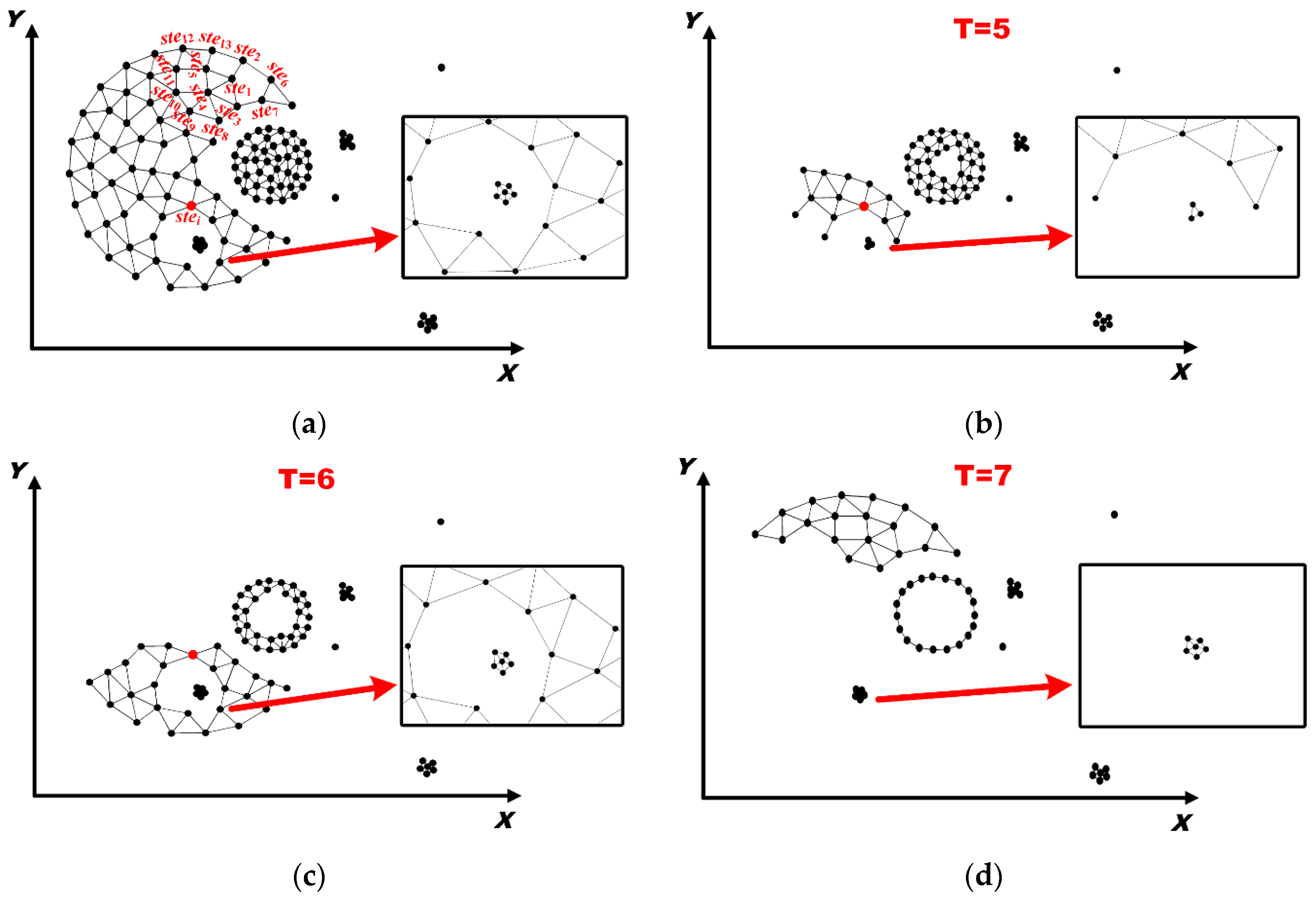
5.1.1. Identification and Removal of I-Long Edges

I-long edges: Given an STE, the corresponding Delaunay triangulation can be built where the I-long edges, denoted as Long_Edges^I(DT), are defined as:

$$Long\_Edge{s}^{\mathrm{I}}\left(DT\right)=\left\{E_i|\left|E_i\right|\ge Mean\left(DT\right)+\frac{Mean\left(DT\right)}{\left|E_i\right|}*Std\left(DT\right)\right\},E_i\in DT$$

(5)

where DT denotes the Delaunay triangulation while E_i is any edge in DT with the length of |E_i|. Mean(DT) and Std(DT) denote the average length of edges in DT and the corresponding standard, respectively.

Here, $\frac{Mean\left(DT\right)}{\left|E_i\right|}$ is an adjusting coefficient that is inversely proportional to the length of edges. Mean(DT) and Std(DT) are both constants, so a longer edge will correspond to a smaller $Mean\left(DT\right)+\frac{Mean\left(DT\right)}{\left|E_i\right|}*Std\left(DT\right)$. As a result, the coefficient $\frac{Mean\left(DT\right)}{\left|E_i\right|}$ is sufficient to identify I-long edges. By removing all I-long edges, a series of sub-graphs for the remaining edges can be obtained, i.e., G⁽¹⁾₁, G⁽¹⁾₂, G⁽¹⁾₃ in Figure 4b. In these sub-graphs the global spatial outliers have been separated from other patterns. II-long edges and III-long edges are further identified below in order to isolate other spatial patterns.

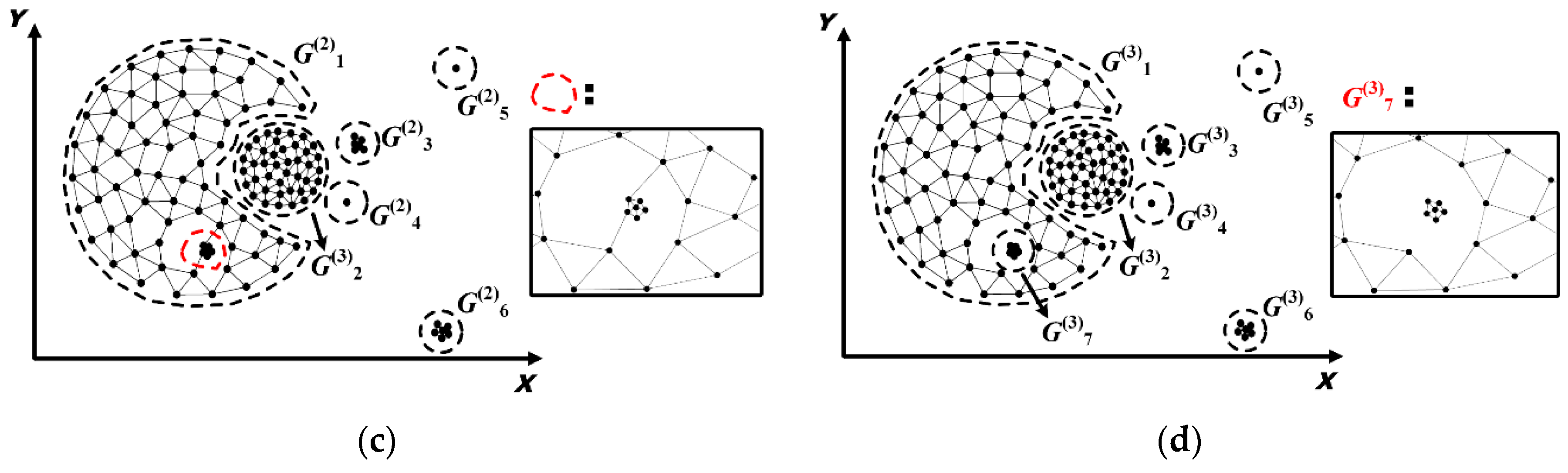
5.1.2. Identification and Removal of II-Long Edges

II-long edges: For any ste_i in sub-graph G⁽¹⁾_k, there are a set of local edges LE_i connecting ste_i with other events. The average length of these local edges and the corresponding standard are denoted as Mean(LE_i) and Std(LE_i), respectively. Further, those II-long edges, denoted as Long_Edges^II(G⁽¹⁾_k), are defined as

$$Long\_Edge{s}^{\mathrm{II}}(G^{(1)}{}_k)=\left\{Local\_Edge(j)|\left|Local\_Edge(j)\right|\ge Mean\left(L{E}_i\right)+\frac{Mean\left(L{E}_i\right)}{\left|Local\_Edge(j)\right|}*Std\left(G^{(1)}{}_k\right)\right\}$$

$$whereLocal\_Edge(j)\in L{E}_{i}andStd(G^{(1)}{}_k)=\frac{{\displaystyle \sum _{i=1}^{\left|G^{(1)}{}_k\right|}Std(L{E}_i)}}{\left|G^{(1)}{}_k\right|}$$

(6)

where Std(G⁽¹⁾_k) represents the average standard of LE_i in G⁽¹⁾_k. Similarly, $\frac{Mean\left(L{E}_i\right)}{\left|Local\_Edge(j)\right|}$ is also an adjusting coefficient to sufficiently identify II-long edges.

After removing all II-long edges in each G⁽¹⁾_k, a new series of sub-graphs can be obtained, i.e., G⁽²⁾₁, G⁽²⁾₂, …, G⁽²⁾₆ in Figure 4c. Those local spatial outliers are further separated. However, some relatively long edges remain in the magnified region in Figure 4c, so the III-long edges that lead the inner spatial outlier region cannot be further divided. These III-long edges need to be identified and dealt with.

5.1.3. Identification and Removal of III-Long Edges

Figure 4c shows that III-long edges are usually located in locally extremely uneven regions, which must therefore be identified first. This problem can be translated into finding those events whose local edges have an extremely large length standard.

Local extremely uneven regions: For any ste_i in G⁽²⁾_k, all events connected with ste_i by local edges LE_i of ste_i are denoted as Con_stei. For local edges LE_j of events in Con_stei, the average and standard value of all Std(LE_j) are denoted as Mean_Std(Con_stei) and Std_Std(Con_stei), respectively, where

$$Mea{n}_{Std}(Co{n}_{st{e}_i})=\frac{{\displaystyle \sum _{j=1}^{\left|Co{n}_{st{e}_i}\right|}Std(L{E}_j)}}{\left|Co{n}_{st{e}_i}\right|}andSt{d}_{Std}\left(Co{n}_{st{e}_i}\right)=\sqrt{\frac{{\displaystyle \sum _{j=1}^{\left|Co{n}_{st{e}_i}\right|}Std(L{E}_j)}}{\left|Co{n}_{st{e}_i}\right|-1}}$$

(7)

Then any locally extremely uneven regions LEUR(G⁽²⁾_k) can be defined as:

$$LEUR(G^{(2)}{}_k)=\left\{st{e}_i|Std(L{E}_i)\ge Mea{n}_{Std}(Co{n}_{st{e}_i})+2\frac{Mea{n}_{Std}(Co{n}_{st{e}_i})}{Std(L{E}_i)}\ast St{d}_{Std}(G^{(2)}{}_k)\right\},st{e}_i\in G^{(2)}{}_k$$

$$whereSt{d}_{Std}(G^{(2)}{}_k)=\frac{{\displaystyle \sum _{i=1}^{\left|G^{(2)}{}_k\right|}St{d}_{Std}\left(Co{n}_{st{e}_i}\right)}}{\left|G^{(2)}{}_k\right|}$$

(8)

III-long edges: For each G⁽²⁾_k, those III-long edges, denoted as Long_Edges^III(G⁽²⁾_k) , are defined as:

$$Long\_Edge{s}^{\mathrm{III}}(G^{(2)}{}_k)=\left\{Local\_Edge(j)|\left|Local\_Edge(j)\right|\ge Mean\left(L{E}_i\right)+2\frac{Mean\left(L{E}_i\right)}{\left|Local\_Edge(j)\right|}*Std\left(G^{(1)}{}_k\right)\right\}$$

$$whereLocal\_Edge(j)\in L{E}_{i}andL{E}_i\in LEUR\left(G^{(2)}{}_k\right)$$

(9)

Equation (9) shows that III-long edges must be located in LEUR(G⁽²⁾_k) and their lengths need to be larger than an indicator that is similar to the one defining II-long edges. Finally, all types of spatial patterns, i.e., G⁽³⁾₁, G⁽³⁾₂, …, G⁽³⁾₇ in Figure 4d, are separated after removing III-long edges. To determine which types of spatial patterns these sub-graphs are, in the following an indicator will be defined that considers the volumes of these sub-graphs.

It should be pointed out that the previous multi-constraint Delaunay triangulation is mainly designed to detect various types of spatial clusters with different shapes and densities [25,26]. The proposed multi-constraint Delaunay triangulation in this study can give a more detailed analysis of the characteristics of edges from different levels, by which various spatial clusters and outliers can be simultaneously detected. For example, III-long edges in Figure 4c are usually located in locally extremely uneven regions, the proposed approach in this paper is able to identify these uneven regions and then extract and delete the hidden III-long edges. This is the main difference from the multi-constrained Delaunay triangulation used before.

5.1.4. Determination of Spatial Patterns

Spatial outliers usually contain very few ste_i and so are defined as those relatively small sub-graphs after the elimination of long edges in the Delaunay triangulation [29]. In addition, those aggregated structures except spatial outliers are defined as spatial clusters in this study. Therefore, following the example of identification of long edges in Section 5.1.1, Section 5.1.2 and Section 5.1.3, the volume of each connected sub-graph will be used to define an indicator for the identification of spatial outliers and clusters.

Spatial clusters and spatial outliers: For each sub-graph G⁽³⁾_k, the volume of G⁽³⁾_k, denoted as Vol(G⁽³⁾_k) is defined as the number of events in G⁽³⁾_k. The mean volume of all the sub-graphs will be employed to separate those small sub-graphs, so amounts of extremely small sub-graphs (with the volume of 1 for example) may seriously obstruct the determination of other relatively small sub-graphs. Therefore, the representative members rvol_i are selected as those volumes that are not equal to each other and gathered together to form a new set RVol. For example, if RVol = {1, 1, 1, 5, 5, 35, 40, 45, 55}, this new set RVol can be obtained and expressed as Rvol = {1, 5, 35, 40, 45, 55}. Then, spatial clusters SC and spatial outliers SA are respectively defined as:

$$SC=\left\{G^{(3)}{}_k|Vol(G^{(3)}{}_k)>Mean\left(RVol\right)-\frac{Vol(G^{(3)}{}_k)}{Mean\left(RVol\right)}*Std\left(RVol\right)\right\}$$

$$SO=\left\{G^{(3)}{}_k|Vol(G^{(3)}{}_k)\le Mean\left(RVol\right)-\frac{Vol(G^{(3)}{}_k)}{Mean\left(RVol\right)}*Std\left(RVol\right)\right\}$$

(10)

where Mean(RVol) and Std(RVol) represent the average value and the standard of the set RVol, respectively. For a smaller sub-graph, the term on the right-hand side of the symbol “≤” in Equation (10) will take a larger value and can therefore be used to identify spatial outliers. Figure 5a,b give the spatial outlier points and regions, respectively, while Figure 5c shows the spatial clusters.

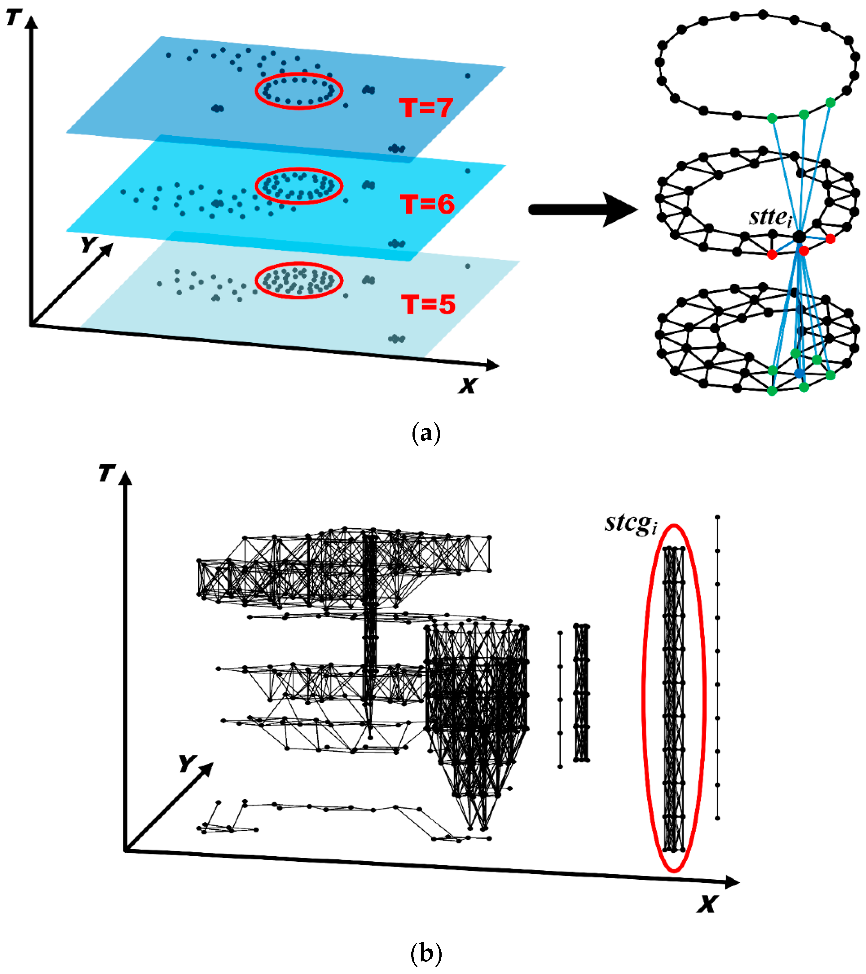
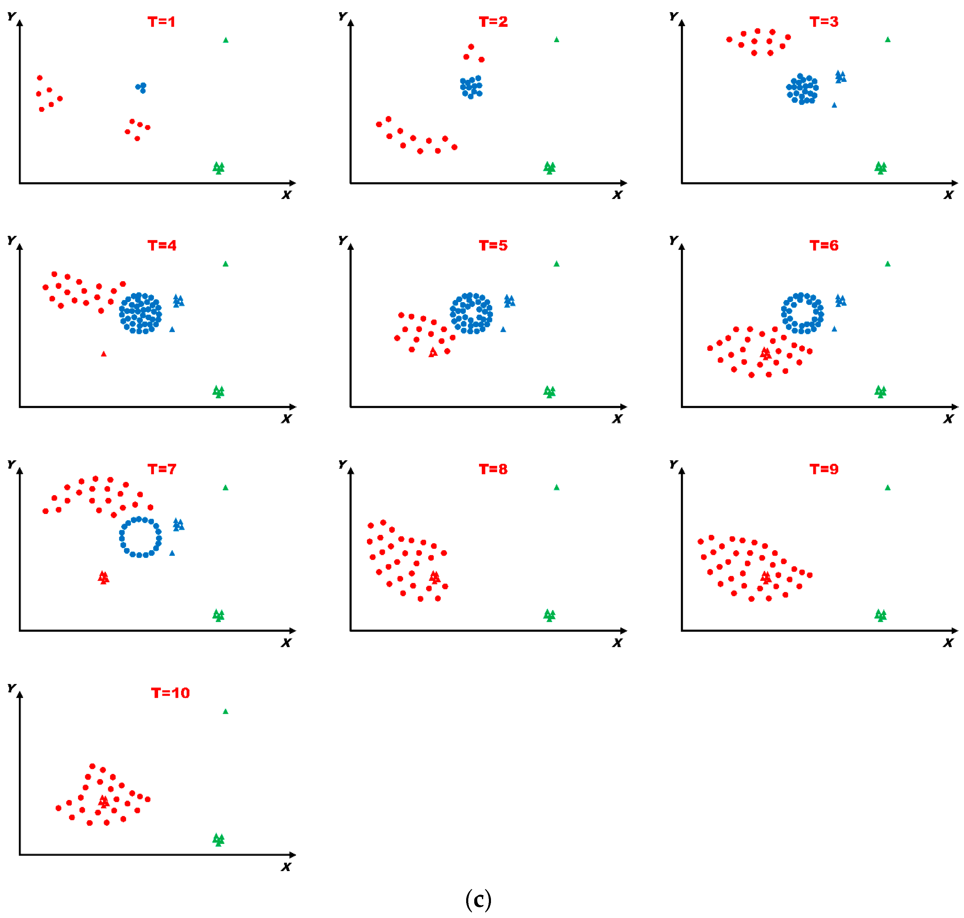
5.2. Discovery of Evolving Spatio-Temporal Patterns

The spatio-temporal distribution patterns for the given time period reflect the evolving process by which the ultimate spatial distribution patterns are formed, i.e., the evolving spatio-temporal patterns. In this section, these will be discovered based on spatio-temporal clustering using the following procedures.

Spatial neighborhoods of STE: Given the spatial patterns obtained from STE, each pattern is a graph made up of a series of spatial Twitter events and the remaining edges in the Delaunay triangulation. For any ste_i, all other events ste_j connected with ste_i form spatial neighborhoods of ste_i, denoted as SN^δ(ste_i), where δ is a threshold representing the number of edges on the shortest path between ste_i and ste_j. Given a δ, SN^δ(ste_i) contains all the spatial Twitter events connected with ste_i by less than or equivalent to δ edges on the shortest path. For example, Figure 6a shows the spatial patterns obtained in Section 5.1. In the figure, ste₁ is connected with ste₂, ste₃, …, ste₅ directly, so ste₂, ste₃, …, ste₅ form SN¹(ste_i). And ste₆, …, ste₁₃ all belong to SN²(ste_i).

Temporal expansion of STE: To determine the time stamp at which each spatial Twitter event occurred, a temporal expansion is performed on STE. Specifically, after the temporal expansion, each member ste_i in STE has m more attributes IsOccur_T_t, where m is the number of time stamps in STTE, that indicate whether a spatial Twitter event occurred at a specific time stamp; if a spatio-temporal Twitter event occurred at T = t at ste_i, then the attribute value of IsOccur_T_t for ste_i, denoted as ste_i·IsOccur_T_t, equals 1 and if not it is 0. For example, Figure 6b–d show the distribution of spatio-temporal Twitter events at T = 5, 6 and 7, respectively. For the ste_i in Figure 6a, it can be obtained that ste_i·IsOccur_T₅ = 1, ste_i·IsOccur_T₆ = 1 and ste_i·IsOccur_T₇ = 0.

Spatial neighborhoods of STTE: Given STTE and STE, for any stte_i located at ste_i’ at time t, if there are spatial Twitter events in SN^δ(ste_i’) with IsOccur_T_t = 1, then those spatio-temporal Twitter events form spatial neighborhoods of stte_i, denoted as SN^δ(stte_i). Figure 6b–d thus show the spatial neighborhoods of STTE at T = 5, 6 and 7, respectively. Here, we assume δ = 1 and two spatio-temporal Twitter events connected by an edge are in the same spatial neighborhood as each other.

Temporal neighborhoods of STTE: Given any stte_i located at ste_i’ at time t and in a time window TW^ε = [t-ε, t-ε+1,…, t-1, t+1,…, t+ε-1, t+ε], other spatio-temporal Twitter events that are also occurring at ste_i’ at time tw_i (tw_i∈TW^ε) are members of the same temporal neighborhood as stte_i, denoted as TN^ε(stte_i). Here, ε is a threshold that determines the range of that temporal neighborhood.

Spatio-temporal neighborhoods of STTE: Given any stte_i and a TW^ε, the spatio-temporal neighborhoods of stte_i, denoted as STN^δ,ε(stte_i), are derived from the following:

(i)

all spatio-temporal Twitter events belonging to SN^δ(stte_i);

(ii)

all spatio-temporal Twitter events belonging to TN^ε(stte_i); and

(iii)

all spatio-temporal Twitter events corresponding to spatial Twitter events in SN^δ(ste_i’) with IsOccur_T_twi(tw_i∈TW^ε)=1, where ste_i’ is the spatial Twitter event of stte_i.

Figure 7a shows the spatio-temporal Twitter events occurring at T = 5–7; the regions surrounded by red circles are produced by the amplification process. Given TW¹ = [t − 1, t + 1], the red, blue and green points represent the above three treatments of STN^1,1(stte_i), respectively.

Spatio-temporal connected graphs of STTE: For each stte_i in STTE, a series of edges can be drawn to connect stte_i and events in STN^δ,ε(stte_i). A graph can be constructed of all the spatio-temporal Twitter events and these edges. All the connected sub-graphs are considered as spatio-temporal connected graphs of STTE, denoted as STCG = {stcg₁, stcg₂, …, stcg_n}. Figure 7b shows the spatio-temporal connected graphs; stcg_i, surrounded by the red ellipse, is an example of a spatio-temporal connected graph.

Evolving spatio-temporal patterns: Given all stcg_i of STTE and the volume of each stcg_i, spatio-temporal clusters (STC), spatio-temporal outlier points (STOP) and spatio-temporal outlier regions (STOR) can be detected using the identification indicator of each of the above spatial patterns. Then, all STC, STOP and STOR consist of evolving spatio-temporal patterns (STEP) of STTE. In other words, STEP describe what kinds of spatio-temporal patterns evolve into each of the spatial distribution patterns. Figure 8 shows the discovered evolving spatio-temporal patterns, where STOP, STOR and STC are shown in Figure 8a,b, respectively, and Figure 8c exhibits the spatial distribution patterns of STE. This suggest several interesting conclusions that can be drawn. For example, in Figure 8c SO₄, located in the lower right corner, belongs to a spatial outlier region but is derived from an STC, i.e., the spatio-temporal cluster represented by green squares in Figure 8b. In addition, the big spatial cluster SC₁ incorporates both STC and STO.

5.3. The Evolving_Pattern_Discovery Algorithm

Based on the related definitions introduced in Section 5.1 and Section 5.2, the proposed algorithm for discovering evolving spatio-temporal patterns from Twitter events can be described as follows:

• Input: Spatio-temporal Twitter events STTE, projected spatial Twitter events STE, threshold δ and ε
• Output: Evolving spatio-temporal patterns

Step I Spatial distribution pattern detection from STE:

(i)

Construct the Delaunay triangulation for STE to obtain the initial spatial proximity graph;

(ii)

Identify and remove inconsistent long edges, i.e., I-long edges, II-long edges and III-long edges, from the Delaunay triangulation;

(iii)

Extract connected sub-graphs and identify spatial clusters and outliers based on the volume of each connected sub-graph.

Step II Discovery of evolving spatio-temporal patterns from STTE:

(i)

Determine the spatial neighborhoods of each spatial Twitter event and the spatial neighborhoods of each spatio-temporal Twitter event based on δ;

(ii)

Construct time windows based on ε and determine the temporal neighborhoods of each spatio-temporal Twitter event;

(iii)

Determine the spatio-temporal neighborhoods of each spatio-temporal Twitter event; and

(iv)

Extract spatio-temporal connected graphs based on the spatio-temporal proximity relationships and identify spatio-temporal clusters and outliers based on the volume of each spatio-temporal connected graph.

In this algorithm, constructing Delaunay triangulation requires O(NlogN), where N is the number of spatial Twitter events. Removing I-long edges and updating the graph require about O(N₁ + N), where N₁ is the number of edges in the Delaunay triangulation. Similarly, the time complexity of removing II-long edges and updating the graph are about O(N₂ + N), where N₂ is the number of the remaining edges after removing I-long edges. The next step, which involves finding extremely uneven regions, removing III-long edges and updating the graph again, require about O(N₃ + 2N), where N₃ is the number of edges located in the extremely uneven regions. Finally, determining the spatio-temporal neighborhoods of spatio-temporal Twitter events and clustering the spatio-temporal connected graphs require about O(N’), where N’ is the number of spatio-temporal Twitter events.

6. Experimental Evaluation and Analysis by Visualization

This section evaluates the effectiveness and practicality of the new framework proposed here by testing it experimentally on a real life dataset. In Section 6.1, the dataset and labels utilized in the experiments are described in detail, after which the experimental analysis is presented in Section 6.2. Finally, Section 6.3 examines the results of the analysis of evolving spatio-temporal patterns.

6.1. Dataset and Labels

The Twitter dataset was purchased from www.datasift.com after a processing of data reduction. It consisted of 10% of all the tweets sent from 21 June 2012 to 31 May 2013 in 10 countries of Latin America and covered the target domain ‘civil unrest’. The tweets from 21 June 2012 to 1 September 2012 in one country, Mexico, was selected to create the case study. It must be noticed that the errors existing in the Twitter data will have an influence on the detection results, so those tweets with significant errors, those published in the ocean for example, have been deleted before performing the experiments. This case study provides an appropriate experimental test for the validation of the framework because ground truth data is available for this scenario. Here the ground truth consists of a group of significant events provided by a Gold Standard Report (GSR) provided by http://www.mitre.org/. Specifically, among the top 100 newspapers in Latin America provided by International Media and Newspapers, the top 3 ones in Mexico, i.e., La Jornada, Reforma and Milenio, were selected to collect news related to ‘civil unrest’ with the input from both the most influential international news outlets and subject matter experts. Events in the news reported by the above two ways would be defined as conflict events. Authoritative news outlets and experts guarantee that the events from GSR are reliable.

For the seed query, 10 tweets related to civil unrest were chosen by users based on the guidance of domain experts to initiate the process [13]. All terms in the 10 tweets were ranked in descending order based on their corresponding DFIDF values [24]. The top 5 terms were selected as the seed terms and included both ‘protest’ and ‘march’. Based on these 5 seed terms, a dynamic query expansion was performed to extract spatio-temporal Twitter events and projected spatial Twitter events. Significant events from the GSR were also projected into the spatio-temporal cube based on their spatial and time tags. Figure 9a,b show the spatio-temporal distribution and spatial projection of both the extracted domain related Twitter events (shown by black points) and the significant events (shown by red triangles) provided by the GSR, respectively.

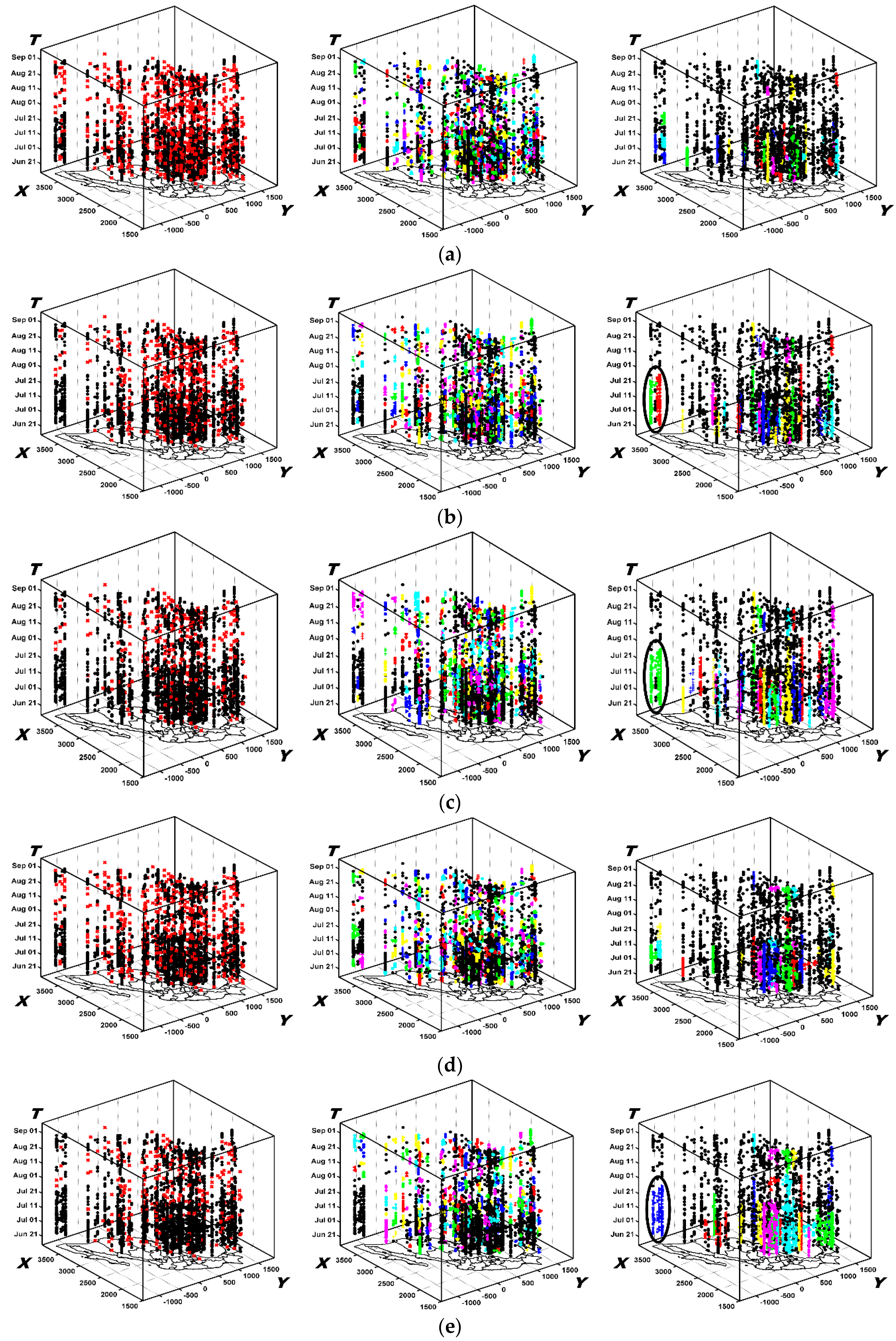
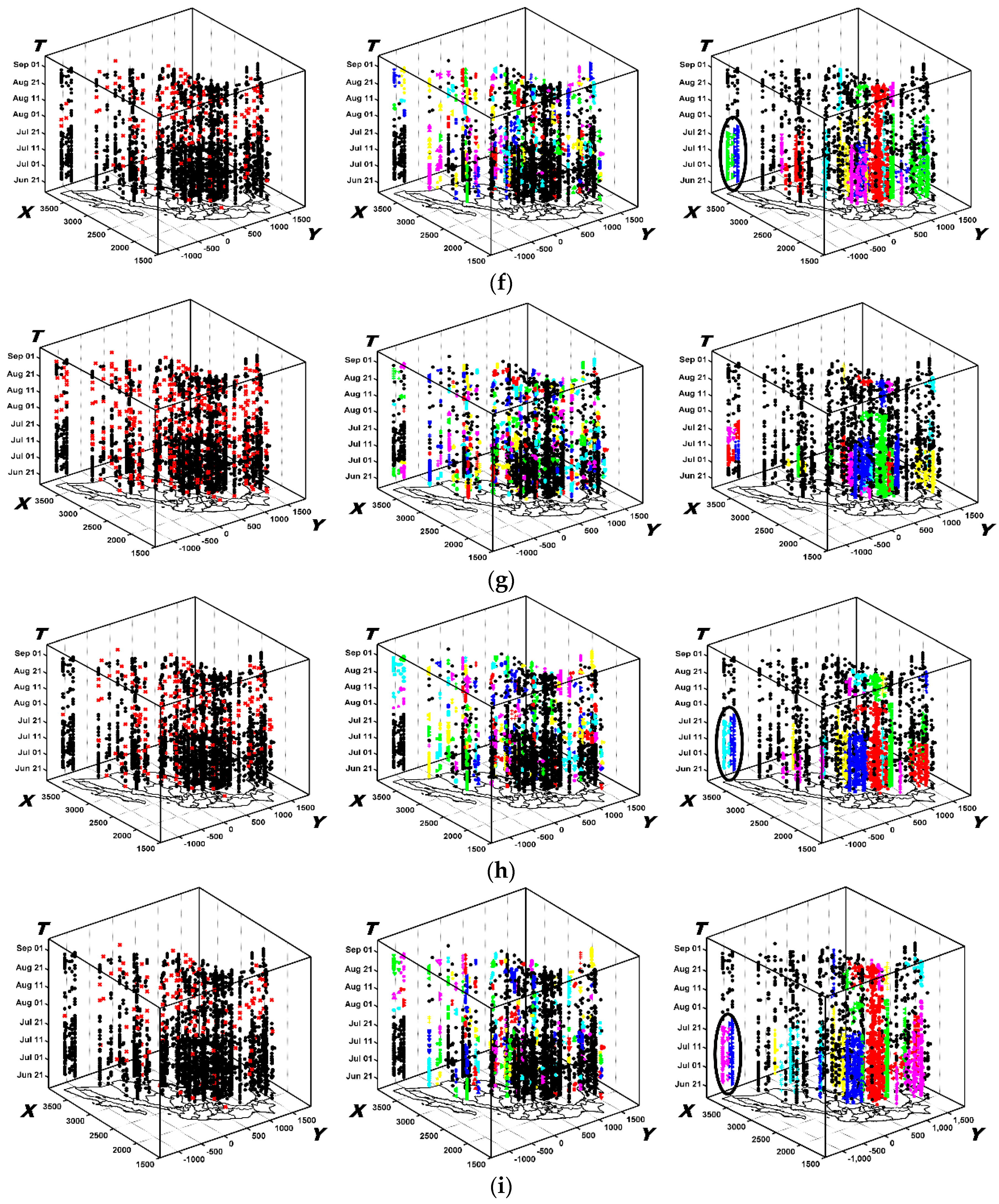
6.2. Experimental Comparisons

In a previous study we demonstrated that dynamic query expansion is an effective tool for extracting domain related Twitter events [13]. Therefore, given the extracted domain related Twitter events, two spatio-temporal point events clustering methods, namely ST-DBSCAN [19] and STSNN [15], are utilized here for comparison. In all experimental results, the symbol “×” represent the spatial and spatio-temporal outlier points. For spatial/spatio-temporal clusters and outlier regions, they are represented by symbols with different shapes and colors.

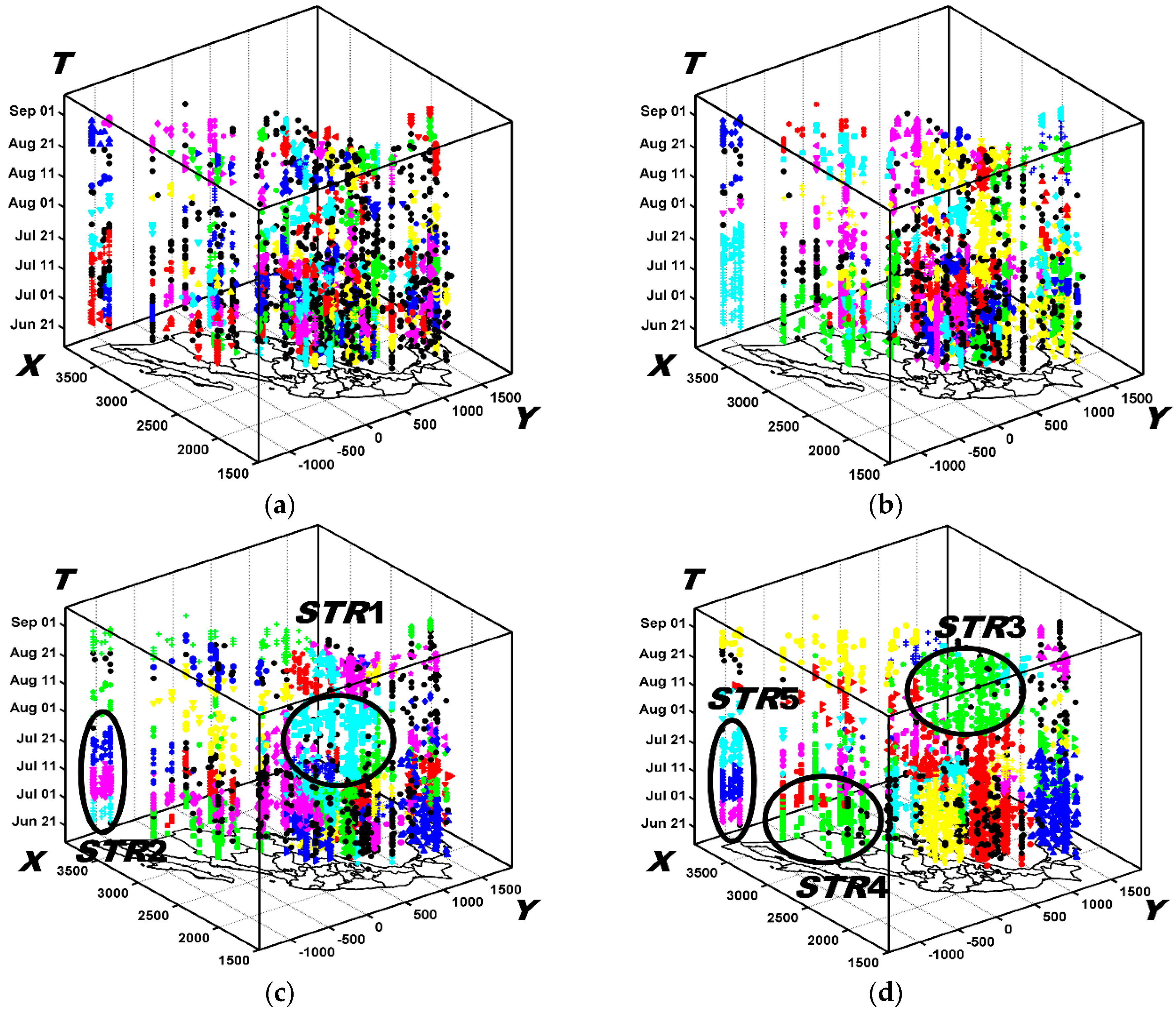
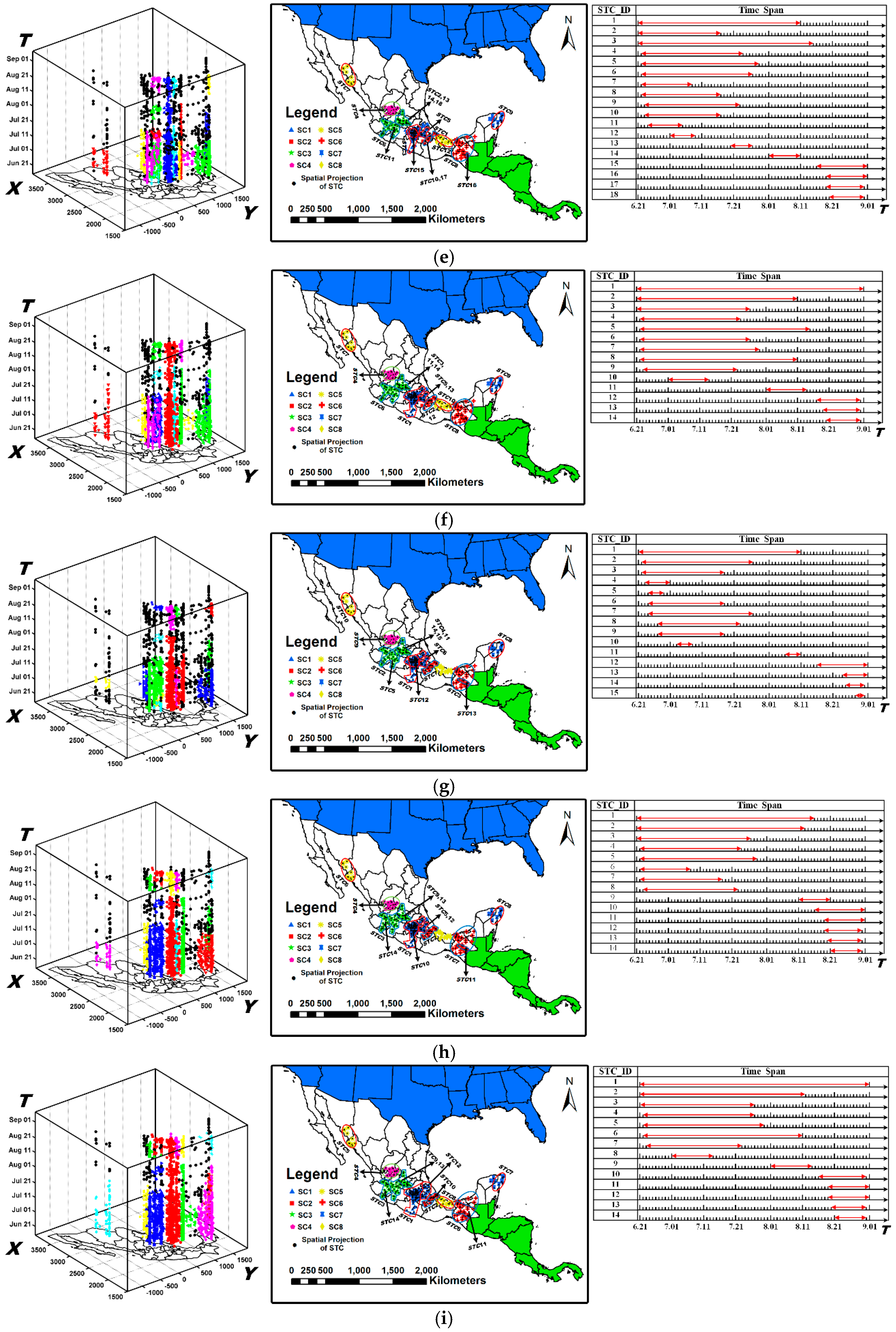
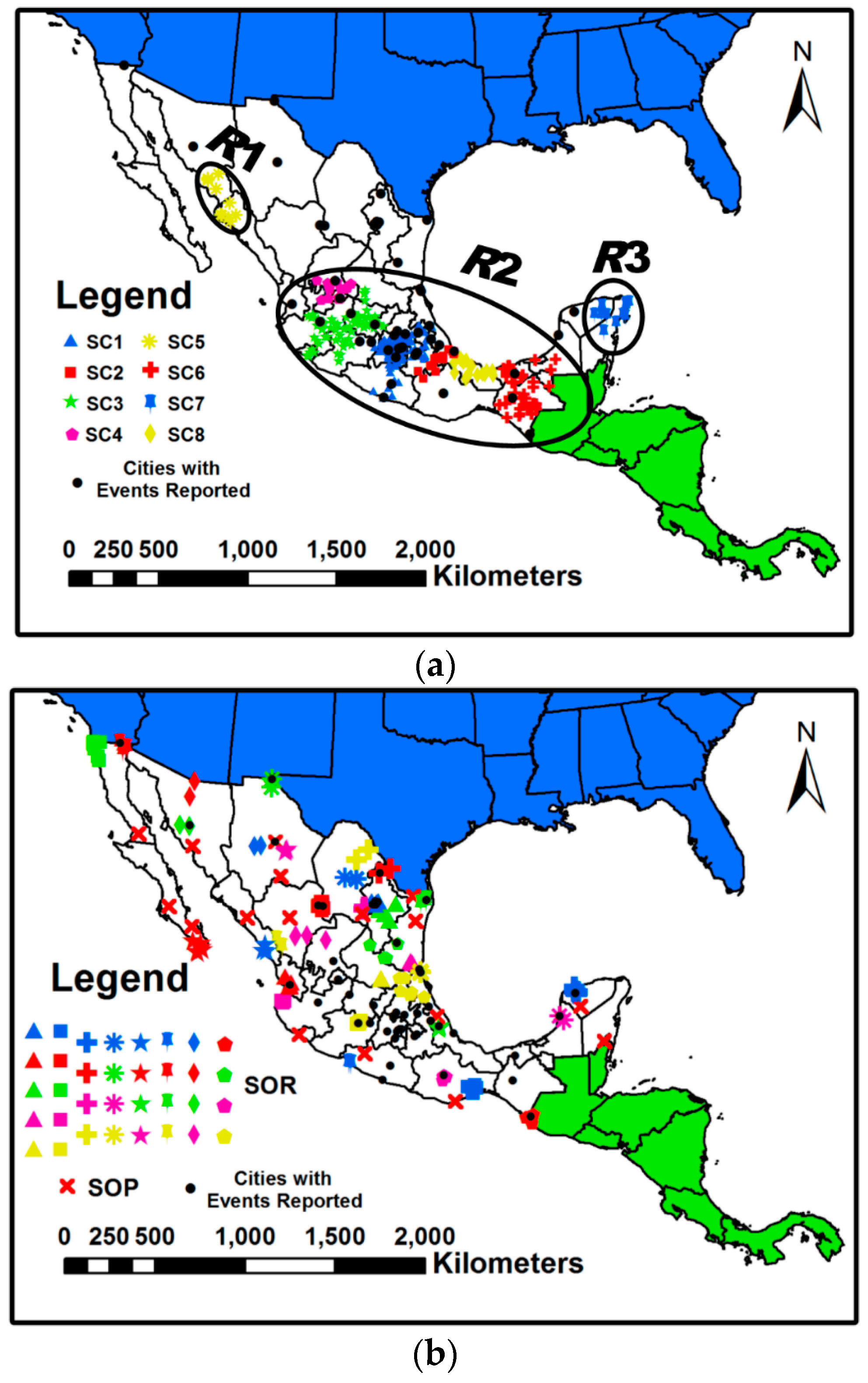
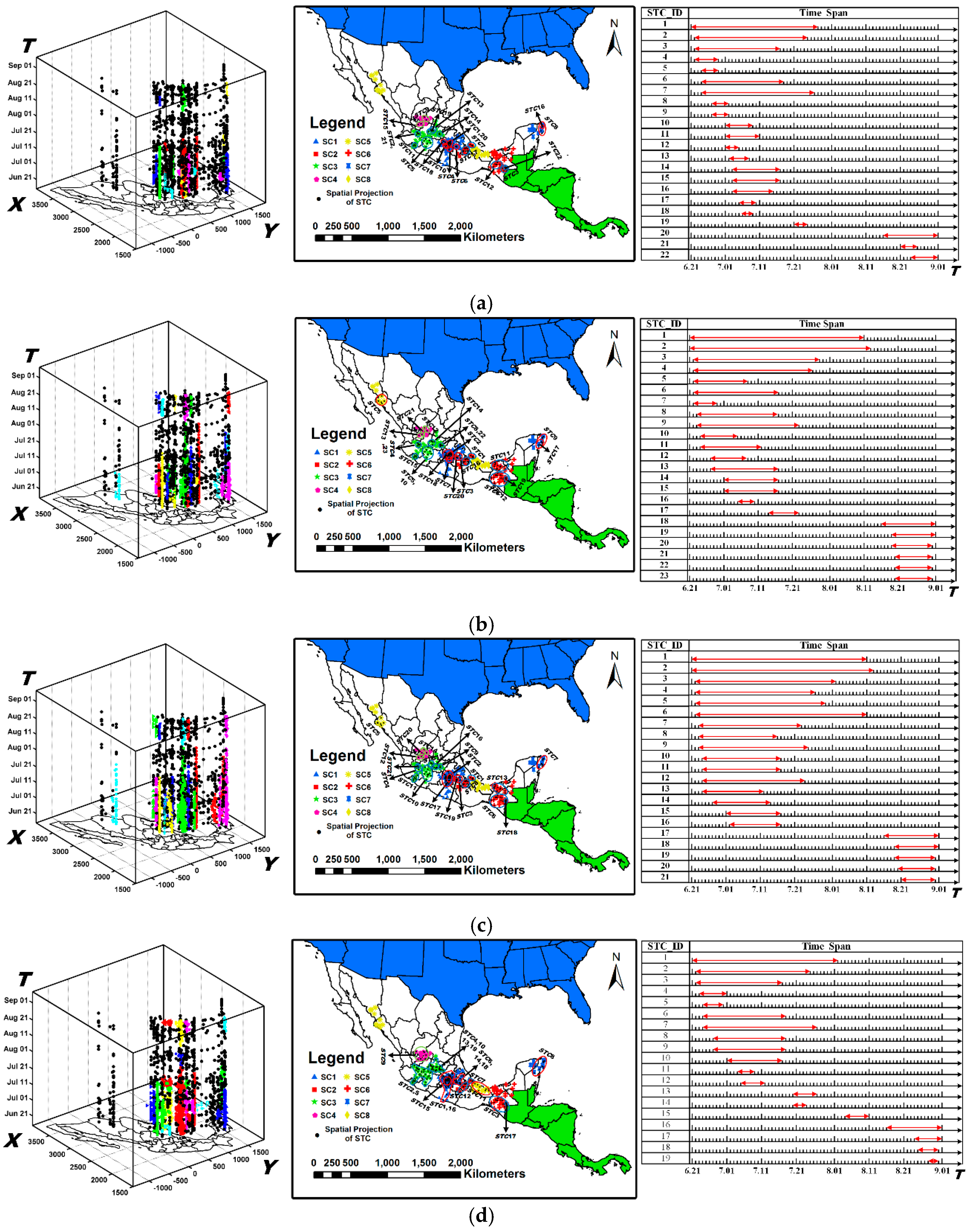
6.2.1. The Results Obtained by the New Method

Figure 10 shows the spatial distribution patterns for STE produced by our new method, where Figure 10a depicts the spatial clusters and Figure 10b both the spatial outlier points and regions. Figure 10a reveals that 8 spatial clusters with different shapes and densities are obtained and that these can be further divided into three main regions, R1, R2 and R3. R1 and R3 are composed of SC5 and SC7, respectively, while R2 covers all the remaining 6 clusters. By comparing these results with the significant events reported in the GSR, these events are mainly distributed in R2, especially in SC1. The spatial outlier points and regions in Figure 10b mainly distribute in the area surrounding R2 and in northern Mexico. One can see that parts of spatial outliers cover all the remaining significant events except those covered by spatial clusters. This indicates that spatial outliers are not just useless noise but can indicate important events as well as spatial clusters.

Based on these spatial distribution patterns, the evolving spatio-temporal patterns can be discovered after setting the thresholds δ and ε. To observe how the results vary for different parameters, δ and ε are assigned values of 1, 2 and 3 to generate a total of 9 pairs of parameters. Figure 11 illustrates all the evolving spatio-temporal patterns for each pair of parameters, where STOP, STOR and STC are shown from left to right, respectively. The figure shows that as δ and ε increase, STOP diminishes while both STOR and STC increase their spatio-temporal ranges. When δ and ε are set as infinity, the spatio-temporal Twitter events whose spatial projections belong to the same spatial distribution pattern are clustered together. Note that because STOP, STOR and STC evolve into their corresponding spatial distribution patterns, each STOP, STOR or STC contain only those spatio-temporal Twitter events located in the same spatial distribution pattern. The proposed method also extracts those spatio-temporal clusters (e.g., those regions signified by ellipses in Figure 11) that form spatial outlier regions. The most significant characteristic of this type of spatio-temporal cluster is that it locally aggregates in the spatial dimension and is continuous in the time dimension.

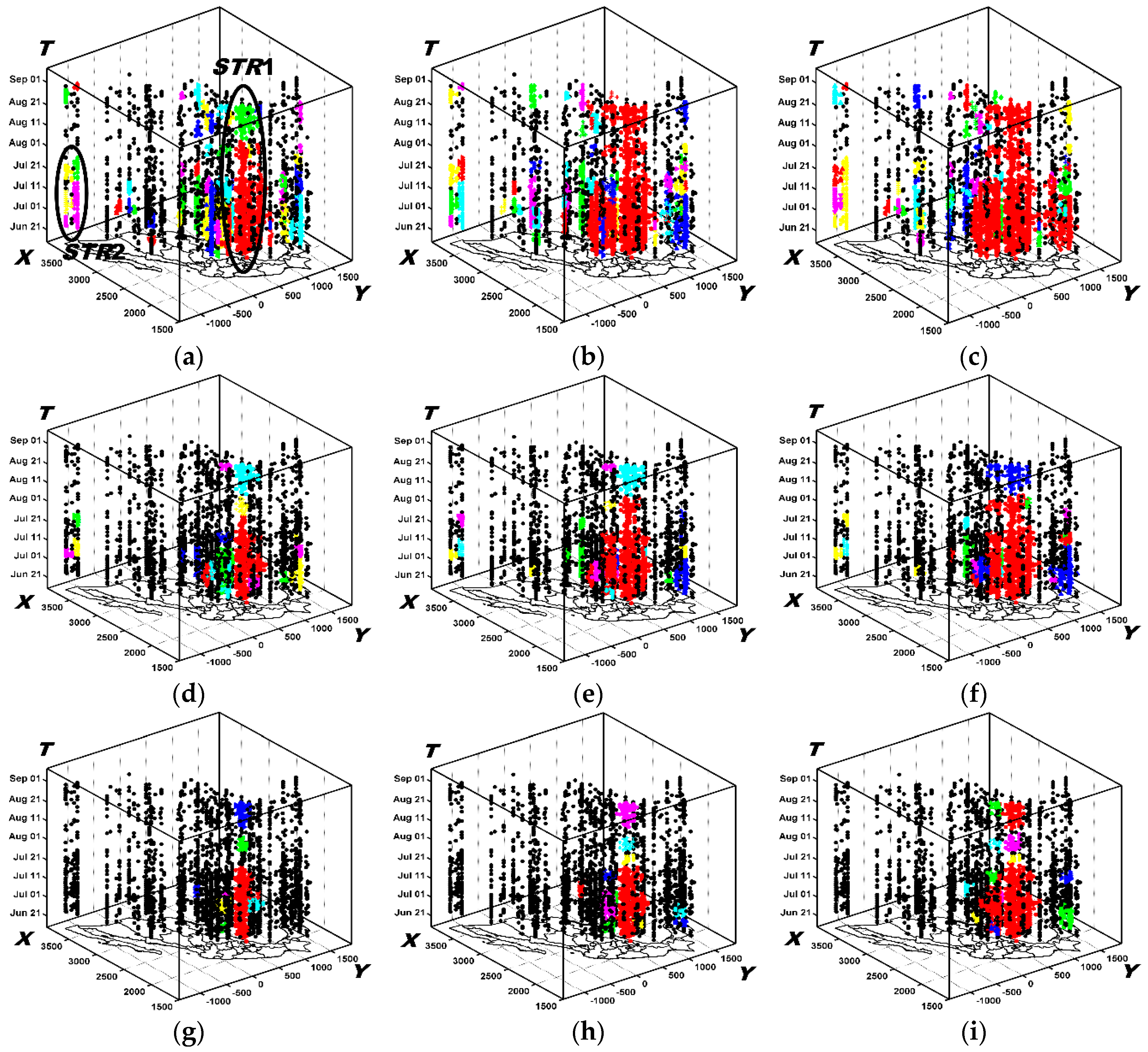
6.2.2. The Results Obtained by ST-DBSCAN

For ST-DBSCAN, the threshold Eps is set as 70 km, 85 km and 100 km, in turn, and MinPts is set as 5, 10 and 15. Repeated experiments revealed that the clustering results are mainly affected by Eps and MinPts, so ΔT is set at 2 days throughout. The results for the 9 sets of parameters are shown in Figure 12, clearly revealing that a larger Eps and a smaller MinPts correspond to larger spatio-temporal clusters. In Figure 12a, two spatio-temporal regions are represented by two black ellipses, labelled STR1 and STR2. As Eps increases and MinPts diminishes, the spatio-temporal cluster in STR1 expands significantly while STR2 is formed by a series of small clusters at all times. ST-DBSCAN only identifies the dense clusters in STR1 and cannot discover the clusters with small spatial ranges but large temporal ranges such as the ones in STR2. However, when Eps is 100 km and MinPts is 5 the spatio-temporal cluster in STR1 contains spatio-temporal Twitter events located in different spatial distribution patterns, as shown in Figure 12c.

6.2.3. The Results Obtained by STSNN

For STSNN, the threshold k is set as 6, 10, 16 and 20 and based on a suggestion by Liu et al. (2014), k_T and MinPts are both set at 0.5k. The threshold ΔT is again set as 2 days. The clustering results for each group of parameters are shown in Figure 13. Here, only a number of discrete small clusters are obtained for k = 6 and 10, but when k is set as 16, a single large spherical spatio-temporal cluster appears in STR1, as shown in Figure 13c. However, this approach suffers from the same problem as ST-DBSCAN, in that both ignore the final spatial distribution patterns of Twitter events. In addition, neither is able to accurately identify those clusters with small spatial ranges and large temporal ranges, such as the one in STR2. In the spatial dimension, this kind of cluster only represents spatial outliers located in a local region collectively, but when considering both space and time indicates that these events take place continuously over a long period of time. It therefore belongs to an important spatio-temporal cluster that is evolving into a spatial outlier region. For k = 20, more significant spatio-temporal cluster are obtained, represented by STR3 and STR4 in Figure 13d. However, the cluster in STR2 of Figure 13c is still not completely detected, for example by STR5 in Figure 13d.

6.3. Analysis of Evolving Spatio-Temporal Patterns

A specific analysis of the evolving spatio-temporal patterns reveals that for the results obtained by the new method and reported in Section 6.2, the emphasis is on analyzing how the spatio-temporal clusters that go on to form spatial clusters vary as the parameters change. Moreover, by focusing on a single set of these results, a more detailed analysis of the evolution of spatio-temporal patterns can be obtained and the results will be compared with the significant events identified from the GSR.

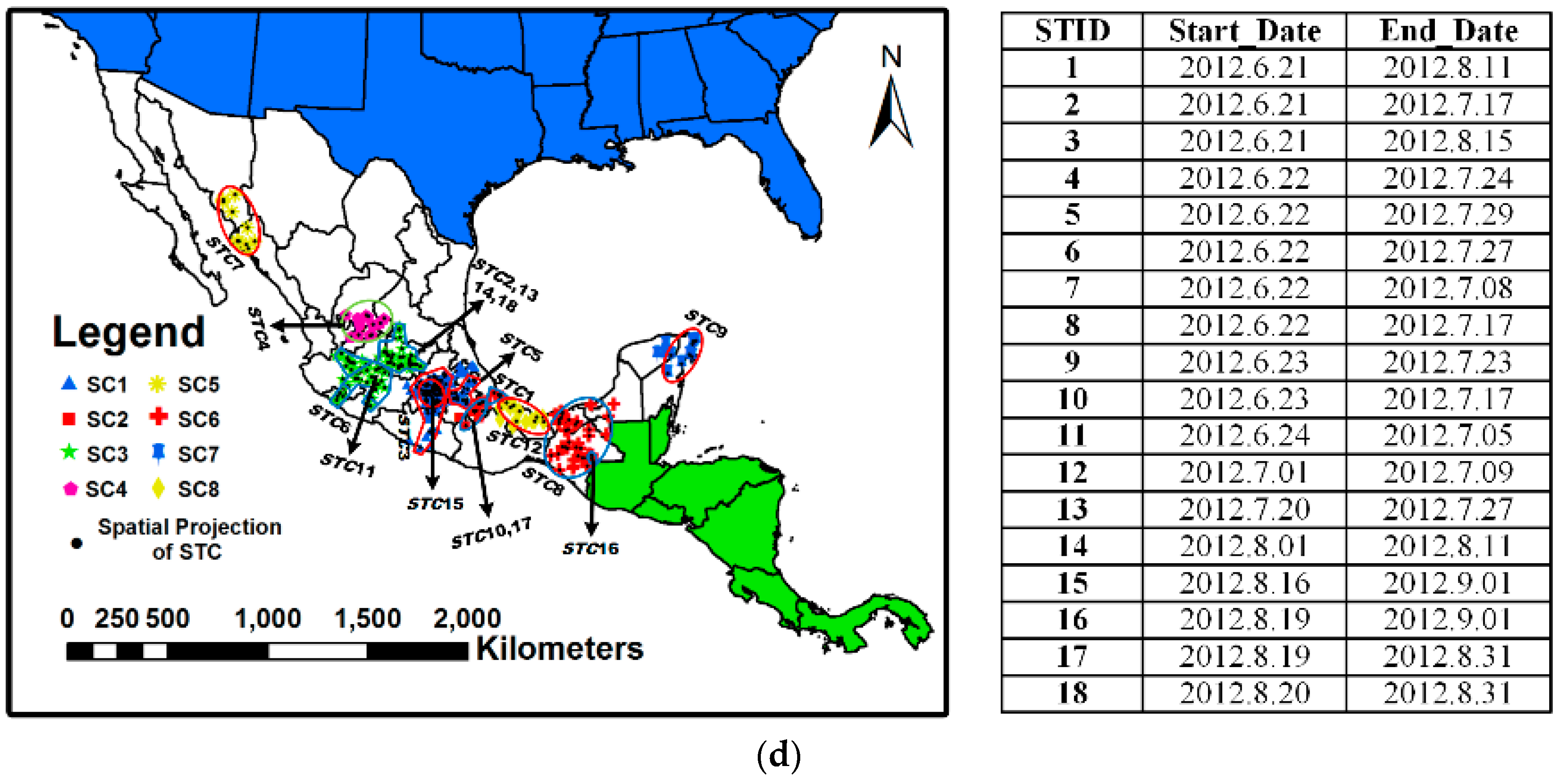
6.3.1. Analysis of Spatio-Temporal Clusters by Our Method

The details of the spatio-temporal clusters that evolve into spatial clusters can be visualized, as shown in Figure 14. For each group of results, the spatio-temporal distribution, spatial locations and time spans (denoted by ‘$\leftrightarrow$’) of the spatio-temporal clusters are shown from left to right. The spatio-temporal clusters with (δ, ε) = (1, 1 days) have small spatial and temporal ranges, as shown in Figure 14a, and are mostly distributed in sporadic spatial clusters, with no significant spatio-temporal clusters forming (SC5 and SC8). In addition, these mainly take place on 2 sets of dates [2012.6.21, 2012.7.28] and [2012.8.16, 2012.9.01], and over a short period of time. As δ increases and ε remains the same, the spatial ranges of these spatio-temporal clusters expand significantly, as can be seen by comparing Figure 14d,g with Figure 14a. Similarly, as ε increases and δ remains the same, each spatio-temporal cluster extends over a longer time period, as shown in Figure 14b,c. δ can also affect the time periods of the spatio-temporal clusters. For example, in Figure 14d, for (δ, ε) = (2, 1 days) not only do the spatial ranges of STC1 in SC1 expand but the time period lengthens from [2012.6.21, 2012.7.28] to [2012.6.21, 2012.8.02]. At the same time, ε can also affect the spatial ranges of the spatio-temporal clusters; when δ remains the same and ε increases to 2 or 3 days, Figure 14b,c reveal that a new spatio-temporal cluster STC5 appears in SC5 that is not visible in Figure 14a.

For the obtained evolving spatio-temporal patterns, δ and ε can to a large extent reflect the outbreak degree of STTE. For example, spatio-temporal clusters with small δ and ε mean those STTE extend only a short distance in the spatial dimension and continuously in the time dimension, but as δ and ε increase, the new members that appear in addition to the original spatio-temporal clusters represent a process of wide and discontinuous extension.

Furthermore, a more detailed analysis illustrates how those spatio-temporal Twitter events evolve into the final spatial distribution patterns by selecting (δ, ε) = (2, 2 days) because of their eclectic nature. Figure 15a,c show the obtained spatio-temporal outlier points, regions and spatio-temporal clusters from left to right, respectively, while the corresponding spatial locations and time periods are shown in Figure 15b,d. The figures reveal 12 spatio-temporal clusters that are in the process of evolving into spatial outliers, mainly located in central and northern Mexico. In Figure 15b, STC1-STC11 is present from late-June to mid- and late-July, while STC12 first appears on 20 August 2012 and lasts until 1 September 2012. A number of spatio-temporal outlier points and regions also form spatial outliers. Spatial clusters are generally evolved into by spatio-temporal clusters, as shown in Figure 15c,d, and most occur between late June to late-July and early-August, with the final four lasting from mid-August to about 31 August 2012. Spatio-temporal outlier points and regions are also implicated in the evolution of spatial clusters, especially those clusters located in central Mexico.

6.3.2. Comparison with Labels

To compare our results with the significant events identified by the GSR, three typical cities where significant numbers of events were reported, namely Ciudad de México, Pachuca de Soto and Monterrey, are selected for further analysis. Figure 16a gives the spatial location of these three cities and the reported dates of significant events are listed in Figure 16b. By combining Figure 16a with Figure 15b,d, one can see that Ciudad de México and Pachuca de Soto both fall within the range of SC1. Ciudad de México also locates in both STC3 and STC15 while Pachuca de Soto locates in STC3. In addition, Monterrey is in STC1 and STC12, both of which form spatial outliers and are represented by ‘$▲$’ in Figure 15b. Figure 16b reveals that significant events were reported in Ciudad de México almost daily throughout July and August, while Pachuca de Soto is reported to have had significant events during mid-July, late-July and on 13 August 2012. STC3 and STC15 in Figure 15d exist during the periods [2012.6.21, 2012.8.15] and [2012.8.16, 2012.9.01], respectively. For Monterrey, significant events were reported during early-July, mid-July and late-August. STC1 and STC12 in Figure 16b exist during the periods [2012.6.21, 2012.8.02] and [2012.8.20, 2012.9.01], respectively. Therefore, the evolving spatio-temporal patterns obtained using the new method are highly consistent with the reported significant events.

7. Conclusions

This paper proposes a framework for discovering evolving domain related spatio-temporal patterns from Twitter data. In our new framework, a dynamic query expansion is employed to extract spatio-temporal Twitter events from the initial Twitter data for a given target domain, after which a spatio-temporal approach that was specifically developed to discover the evolving spatio-temporal patterns of the domain related Twitter events is applied. By utilizing Twitter datasets in Mexico for the domain of civil unrest, an experimental comparison with ST-DBSCAN and STSNN was conducted to illustrate the effectiveness of our proposed method and its practicality demonstrated by comparing the results obtained by our method with the significant events identified in the Gold Standard Report.

In summary, the GSR only collected those dates when events reached their climax, but these events were usually preceded by a period during which minor conflicts escalated and were followed by the subsequent fallout from the event. The evolving spatio-temporal patterns for the Twitter events can reflect the characteristic of reported events based on the reactions of the human observers and participants. It would thus be helpful to refine this approach further in order to accurately predict the evolution process for different types of events in each representative region (i.e., those spatial clusters and outliers). However, to effectively perform the geographical analysis of Big Data, such as social media data focused on in this study, the data quality cannot be ignored because it is very common that there possibly contain numerous errors in the initial data. Also, the social media data is usually biased from the population, so it is a challenge that the bias should be remedied to make the data to reflect the spatio-temporal patterns correctly [30]. Therefore, our future work will focus on the analysis of quality, incompletion and uncertainty for Twitter data and further modifying our proposed methods. The modifiable temporal unit problem (MTUP) problem can impact the detection results, so how to select optimal width of time window by considering the MTUP problem and specific practical applications will also be investigated in the future [31,32]. As the variety of spatio-temporal Big Data, there is a challenge of mining potential spatio-temporal patterns from multiple datasets across different domains with different representations, distributions, scales, densities and so on [33,34]. In addition, methods of geographical visualization should be developed to present the complicated analyzed results to users vividly and comprehensibly.

References

1. Java, A.; Song, X.; Finin, T.; Tseng, B. Why we twitter: Understanding microblogging usage and communities. In Proceedings of the 9th WebKDD and 1st SNAKDD 2007 Workshop on Web Mining and Social Network Analysis, San Jose, CA, USA, 12–15 August 2007; pp. 56–65.
2. Cheng, A.; Mark, E.; Harshdee, S. Inside Twitter: An in-Depth Look Inside the Twitter World; SYSOMOS: Toronto, ON, Canada, June 2009. [Google Scholar]
3. De Albuquerque, J.P.; Herfort, B.; Brenning, A.; Zipf, A. A geographic approach for combining social media and authoritative data towards identifying useful information for disaster management. Int. J. Geogr. Inf. Sci. 2015. [Google Scholar] [CrossRef]
4. Heverin, T.; Zach, L. Microblogging for crisis communication: Examination of twitter use in response to a 2009 violent crisis in Seattle-Tacoma, Washington area. In Proceedings of the 7th International ISCRAM Conference, Seattle, WA, USA, 2–5 May 2010.
5. Pan, B.; Zheng, Y.; Wilkie, D.; Shahabi, C. Crowd sensing of traffic anomalies based on human mobility and social media. In Proceedings of the 21st ACM SIGSPATIAL International Conference on Advances in Geographic Information Systems, Orlando, FL, USA, 5–8 November 2013; pp. 334–343.
6. Chew, C.; Eysenbach, G. Pandemics in the age of Twitter: Content analysis of Tweets during the 2009 H1N1 outbreak. PLoS ONE 2009, 5, e14118. [Google Scholar] [CrossRef] [PubMed]
7. Ramage, D.; Dumais, S.; Liebling, D. Characterizing microblogs with topic models. In Proceedings of the 4th International AAAI Conference on Weblogs and Social Media, Washington, DC, USA, 23–26 May 2010; pp. 130–137.
8. Markman, V. Unsupervised discovery of fine-grained topic clusters in Twitter posts. Pap. AAAI Workshop Anal. Microtext 2011, WS-11–05, 32–37. [Google Scholar]
9. Fujisaka, T.; Lee, R.; Sumiya, K. Detection of unusually crowded places through micro-blogging sites. In Proceedings of 2010 IEEE 24th International Conference on Advanced Information Networking and Applications Workshops, Perth, Australia, 20–23 April 2010; pp. 467–472.
10. Lee, R.; Wakamiya, S.; Sumiya, K. Discovery of unusual regional social activities using geo-tagged microblogs. World Wide Web 2011, 14, 321–349. [Google Scholar] [CrossRef]
11. Chae, J.; Thom, D.; Bosch, H.; Jang, Y.; Maciejewski, R. Spatiotemporal social media analytics for abnormal event detection an examination using seasonal-trend decomposition. In Proceedings of the 2012 IEEE Conference on Visual Analytics Science and Technology (VAST), Seattle, WA, USA, 14–19 October 2012; pp. 143–152.
12. Cheng, T.; Wicks, T. Event detection using Twitter: A spatio-temporal approach. PLoS ONE 2014, 9, e97807. [Google Scholar] [CrossRef] [PubMed]
13. Zhao, L.; Chen, F.; Dai, J.; Hua, T.; Lu, C.-T.; Ramakrishnan, N. Unsupervised spatial event detection in targeted domains with applications to civil unrest modeling. PLoS ONE 2014, 9, e110206. [Google Scholar] [CrossRef] [PubMed]
14. Bakillah, M.; Li, R.Y.; Liang, S.H. Geo-located community detection in Twitter with enhanced fast-greedy optimization of modularity: The case study of typhoon Haiyan. Int. J. Geogr. Inf. Sci. 2014. [Google Scholar] [CrossRef]
15. Liu, Q.; Deng, M.; Bi, J.; Yang, W. A novel method for discovering spatio-temporal clusters of different sizes, shapes and densities in the presence of noise. Int. J. Digit. Earth 2014, 7, 138–157. [Google Scholar] [CrossRef]
16. Blei, D.; Ng, A.; Jordan, M. Latent Dirichlet Allocation. J. Mach. Learn. Res. 2003, 3, 993–1022. [Google Scholar]
17. Signorini, A.; Segre, A.M.; Polgreen, P.M. The use of Twitter to track levels of disease activity and public concern in the US during the influenza A H1N1 pandemic. PLoS ONE 2011, 6, e19467. [Google Scholar] [CrossRef] [PubMed]
18. Chakrabarti, D.; Punera, K. Event summarization using tweets. In Proceedings of the 5th International AAAI Conference on Weblogs and Social Media, Barcelona, Spain, 17–21 July 2011; pp. 66–73.
19. Wang, M.; Wang, A.; Li, A. Mining spatial-temporal clusters from geo-database. Lect. Notes Artif. Intell. 2006, 4093, 263–270. [Google Scholar]
20. Cheng, T.; Li, Z. A multiscale approach for spatio-temporal outlier detection. Trans. GIS 2006, 10, 253–263. [Google Scholar] [CrossRef]
21. Wu, E.; Liu, W.; Chawla, S. Spatio-temporal outlier detection in precipitation data. Knowl. Discov. Sens. Data 2010, 5840, 115–133. [Google Scholar]
22. Kulldorff, M.; Heffernan, R.; Hartman, J.; Assunção, R.; Mostashari, F. A space-time permutation scan statistic for disease outbreak detection. PLoS Med. 2005, 2, e59. [Google Scholar] [CrossRef] [PubMed] [Green Version]
23. Liu, P.; Zhou, D.; Wu, N. VDBSCAN: Varied density based spatial clustering of application with noise. In Proceedings of 2007 International Conference on Service Systems and Service Management, Chengdu, China, 9–11 June 2007; pp. 528–531.
24. Weng, J.; Lee, B.S. Event detection in Twitter. In Proceedings of the 5th International AAAI Conference on Weblogs and Social Media, Barcelona, Spain, 17–21 July 2011; pp. 401–408.
25. Estivill-Castro, V.; Lee, I. Argument free clustering for large spatial point-data sets. Comput. Environ. Urban Syst. 2002, 26, 315–334. [Google Scholar] [CrossRef]
26. Deng, M.; Liu, Q.; Cheng, T.; Shi, Y. An adaptive spatial clustering algorithm based on Delaunay triangulation. Comput. Environ. Urban Syst. 2011, 35, 320–332. [Google Scholar] [CrossRef]
27. Jiang, M.-F.; Tseng, S.-S.; Su, C.-M. Two-phase clustering process for outliers detection. Pattern Recognit. Lett. 2001, 22, 691–700. [Google Scholar] [CrossRef]
28. Al-Zoubi, M.B.; Al-Dahoud, A.A.; Yahya, A. New outlier detection method based on fuzzy clustering. WSEAS Trans. Inf. Sci. Appl. 2010, 7, 681–690. [Google Scholar]
29. Shi, Y.; Deng, M.; Yang, X.; Liu, Q. Adaptive detection of spatial point event outliers using multilevel constrained Delaunay triangulation. Comput. Environ. Urban Syst. 2016. [Google Scholar] [CrossRef]
30. Wang, J.; Ge, Y.; Li, L.; Meng, B.; Wu, J.; Bo, Y.; Du, S.; Liao, Y.; Hu, M.; Xu, C. Spatiotemporal data analysis in geography. Acta Geogr. Sin. 2014, 69, 1326–1345. [Google Scholar]
31. Cheng, T.; Adepeju, M. Modifiable temporal unit problem (MTUP) and its effect on space-time cluster detection. PLoS ONE 2014, 9, e100465. [Google Scholar] [CrossRef] [PubMed]
32. Huang, Q.; Wong, D.W.S. Modeling and visualizing regular human mobility patterns with uncertainty: An example using Twitter data. Ann. Assoc. Am. Geogr. 2015, 105, 1179–1197. [Google Scholar] [CrossRef]
33. Zheng, Y. Methodologies for cross-domain data fusion: An overview. IEEE Trans. Big Data 2015, 1, 16–34. [Google Scholar] [CrossRef]
34. Zheng, Y.; Zhang, H.; Yu, Y. Detecting collective anomalies from multiple spatio-temporal datasets across different domains. In Proceedings of the 23rd ACM SIGSPATIAL International Conference on Advances in Geographic Information Systems, Bellevue, WA, USA, 3–6 November 2015; pp. 1–10.
Figure 1. A real-world example of spatio-temporal Twitter events.
Ijgi 05 00193 g001
Figure 2. A simulated dataset of spatio-temporal point events with 10 time stamps. (a) spatio-temporal distribution of the dataset viewed from four different perspectives; (b) spatial projection of spatio-temporal point events for all time stamps; (c) spatial projection of spatio-temporal point events for individual time stamps.
Ijgi 05 00193 g002aIjgi 05 00193 g002b
Figure 3. The proposed framework for discovering evolving patterns in geo-tagged Twitter events.
Ijgi 05 00193 g003
Figure 4. The process of imposing multi-constraints on Delaunay triangulation. (a) the initial Delaunay triangulation; (b) the result of imposing constraints at the macro level; (c) the result of imposing constraints at the middle level; (d) the result of imposing constraints at the micro level.
Ijgi 05 00193 g004aIjgi 05 00193 g004b
Figure 5. The process of identifying spatial clusters and spatial outliers. (a) spatial outlier points; (b) spatial outlier regions; (c) spatial outlier clusters.
Ijgi 05 00193 g005
Figure 6. The construction of spatial proximity relationships. (a) spatial Twitter events covering the whole time period; (bd) spatial Twitter events at T = 5, T = 6 and T = 7, respectively.
Ijgi 05 00193 g006
Figure 7. The construction of spatial proximity relationships. (a) spatio-temporal Twitter events from T = 5 to T = 7; (b) spatio-temporal connecting graphs.
Ijgi 05 00193 g007
Figure 8. Evolving spatio-temporal patterns of STTE and spatial distribution patterns of STE. (a) Spatio-temporal outliers; (b) Spatio-temporal clusters; (c) the spatial distribution patterns of STE. In each figure, different symbols represent different STO or STC except for black points.
Ijgi 05 00193 g008
Figure 9. The STTE related to civil unrest in Mexico from June 21 to September 1. (a) spatio-temporal distribution viewed from two different perspectives; (b) the corresponding STE obtained by spatial projection of the spatio-temporal Twitter events.
Ijgi 05 00193 g009
Figure 10. The spatial distribution patterns for STE. (a) spatial clusters; (b) spatial outliers. SOP and SOR represent spatial outlier points and regions respectively.
Ijgi 05 00193 g010
Figure 11. The evolving spatio-temporal patterns of STTE discovered by the proposed method. (a) δ = 1, ε = 1; (b) δ = 1, ε = 2; (c) δ = 1, ε = 3; (d) δ = 2, ε = 1; (e) δ = 2, ε = 2; (f) δ = 2, ε = 3; (g) δ = 3, ε = 1; (h) δ = 3, ε = 2; (i) δ = 3, ε = 3.
Ijgi 05 00193 g011aIjgi 05 00193 g011b
Figure 12. The spatio-temporal clusters discovered by ST-DBSCAN. (a) Eps = 70, MinPts = 5, ΔT = 2; (b) Eps = 85, MinPts = 5, ΔT = 2; (c) Eps = 100, MinPts = 5, ΔT = 2; (d) Eps = 70, MinPts = 10, ΔT = 2; (e) Eps = 85, MinPts = 10, ΔT = 2; (f) Eps = 100, MinPts = 10, ΔT = 2; (g) Eps = 70, MinPts = 15, ΔT = 2; (h) Eps = 85, MinPts = 15, ΔT = 2; (i) Eps = 100, MinPts = 15, ΔT = 2.
Ijgi 05 00193 g012
Figure 13. The spatio-temporal clusters discovered by STSNN. (a) k = 6, kT = 3, MinPts = 3, ΔT = 2; (b) k = 10, kT = 5, MinPts = 5, ΔT = 2; (c) k = 16, kT = 8, MinPts = 8, ΔT = 2; (d) k = 20, kT = 10, MinPts = 10, ΔT = 2.
Ijgi 05 00193 g013
Figure 14. The spatio-temporal clusters in STTE that form the spatial clusters in STE and their spatial locations and time periods. (a) δ = 1, ε = 1; (b) δ = 1, ε = 2; (c) δ = 1, ε = 3; (d) δ = 2, ε = 1; (e) δ = 2, ε = 2; (f) δ = 2, ε = 3; (g) δ = 3, ε = 1; (h) δ = 3, ε = 2; (i) δ = 3, ε = 3.
Ijgi 05 00193 g014aIjgi 05 00193 g014b
Figure 15. The evolving spatio-temporal patterns discovered for STTE with the parameters δ = 2, ε = 2. (a,b) the evolving spatio-temporal patterns of spatial outliers and their spatial locations and time ranges; (c,d) the evolving spatio-temporal patterns of spatial clusters and their spatial locations and time ranges.
Ijgi 05 00193 g015aIjgi 05 00193 g015b
Figure 16. Three cities reporting numerous significant events. (a) geo-location of the three cities; (b) reporting dates of significant events for the three cities.
Ijgi 05 00193 g016aIjgi 05 00193 g016b