Article

A Long Baseline Three Carrier Ambiguity Resolution with a New Ionospheric Constraint

1
State Key Laboratory of Geodesy and Earth’s Dynamics, Institute of Geodesy and Geophysics, Chinese Academy of Sciences, Wuhan 430077, China
2
University of Chinese Academy of Sciences, No. 19A Yuquan Road, Beijing 100049, China
3
Shandong Women’s University, Jinan 250300, China
*
Author to whom correspondence should be addressed.
ISPRS Int. J. Geo-Inf. 2016, 5(11), 198; https://0-doi-org.brum.beds.ac.uk/10.3390/ijgi5110198
Submission received: 23 August 2016 / Revised: 25 October 2016 / Accepted: 27 October 2016 / Published: 1 November 2016
(This article belongs to the Special Issue Recent Advances in Geodesy & Its Applications)

Abstract

:
Global navigation satellite sensors can transmit three frequency signals. When the classical three-carrier ambiguity resolution (TCAR) is applied to long baselines of hundreds of kilometres, the narrow-lane integer ambiguity resolution (IAR) is affected by the remaining double-differenced (DD) ionospheric delays. As such, large amounts of observational data are typically needed for successful recovery. To strengthen ionospheric delays, we analysed the combination of three frequency signals and a new ambiguity-free ionospheric combination where the least amount of noise is defined, which is enhanced with epoch-differenced ionospheric delays to provide better absolute ionospheric delay and temporal change. To optimize ionosphere estimations, we propose defining the optimal smoothing length, and also propose a strategy to diagnose wrongly determined ionospheric estimations. With such ionospheric information, we can obtain the ionosphere-weighted model by incorporating the ionospheric information to the geometry-based model and use the real triple-frequency observations to evaluate our method. Our results show that the precision of ionospheric estimations from our new ionospheric model is 25% higher than that from the current combination method and that it can provide real-time smoothed ionospheric delay with magnitudes defined to the nearest centimetre. Additionally, using ionospheric estimation as a constraint, the ionosphere-weighted model requires 20% less time to generate the first-fixed solution (TFFS) than the geometry-based model.

1. Introduction

Modern navigation satellite systems can transmit three or more frequency signals. GPS and QZSS introduced the L5 signal, in addition to the current L1 and L2 signals. Chinese Beidou satellites can transmit L2, L7 and L6 signals, and Galileo was designed to provide signals centred at L1, E6, E5B and E5A. The third frequency is close to the second frequency, which creates favourable conditions for directly fixing extra wide-lane (EWL) ambiguity and further achieving wide-lane (WL) and narrow-lane (NL) ambiguity resolutions (AR). Thus, using triple-frequency signals to improve the efficiency and reliability of AR in long baselines has become an active research topic.
Triple-frequency combinations can be divided into EWL, WL and NL combinations according to their wavelength, varying from longest to shortest. The EWL combination has the longest wavelength, and its magnitude is many times larger than that of the combination noise and the ionospheric residual. Employing the least squares (LS) algorithm, the EWL ambiguity can be determined by using the single epoch observable [1]. Combining the resolved EWL ambiguity with the original phase observations and pseudorange observations to resolve WL ambiguity, the success rate of such WL resolutions can reach 99% in epoch-wise data processing [2,3]. Compared to the EWL and WL resolutions, the narrow-lane IAR is more easily affected by the ionospheric residual and the combination noise because its wavelength is small [2]. As such, extensive research has been conducted in this area, and some modified methods have been developed.
One typical resolution is to select geometry-free and ionosphere-free (GIF) models characterized by smaller ionospheric effects and a lack of geometry coupling. A new combination selection strategy based on ionospheric terms with smaller total noise levels was proposed for the GPS, Galileo and BDS systems [4]. Similarly, combination sets of Galileo’s three frequencies were also proposed with smaller ratios between the combination ionospheric delay and wavelength, as well as their corresponding combination noise varying from 0.1 to 0.2 cycles [5,6]. However, for the many proposed “virtual” ionosphere-free (IF) combinations, most proposals reduce the ionospheric effect but do not actually remove it. Thus, these NL ambiguity resolutions are still affected by the ionospheric effect when the ionosphere is active or when these algorithms are applied to long baselines. In some of the special combination methods, the estimated coefficients fully satisfy the GIF conditions. However, these combinations lead to a stable NL ambiguity root mean square (RMS) value of approximately 3.5 cycles [2]. Nearly 200 observations of float NL estimates must be smoothed for the NL resolution to achieve a small estimation error of 0.25 cycles, and the number of necessary smoothed NL estimates will be decreased if the noise level is decreased.
To overcome the aforementioned deficiencies in GIF models, many researchers have extended the concepts and algorithms of TCAR to allow for their use with the geometry-based model [4,7,8,9,10,11,12]. These studies involve the use of large numbers of unknown parameters in the estimation process, and the convergence of these unknowns is time consuming. To address the issue of ionospheric delays, some ionosphere-free techniques have been used; however, these approaches sacrifice the integer nature of the ambiguity and make it difficult to find integer ambiguity candidates [13]. Recent experiments have verified that DD ionospheric delays can be treated as unknown parameters accompanied with coordinates and ambiguities. In turn, the advantage becomes more significant, especially when this type of resolution is applied to long baselines [14]. To further shorten the time required for successful IAR, some scholars propose using external ionospheric constraints to strength ionospheric estimates. One way to accurately estimate the DD ionospheric delay is to interpolate the ionospheric delay from the permanent GNSS network. The magnitude of precision of the ionospheric estimation can be defined to the nearest centimetre. Such a wide GNSS network is not available in most places, especially in rural and marine areas [15]. The global ionospheric TEC map (GIM) can also provide an estimation of ionospheric delay, and its precision is 2–8 TECu, which hardly satisfies the requirement of being treated as an ionospheric constraint [16]. In addition, the DD ionospheric delay can also be estimated by combining the raw observables and the resolved ambiguities. The precision of ionospheric estimates can achieve magnitudes defined to the nearest centimetre only after estimates from tens of epochs are smoothed [17]. Compared with the operation of extracting ionospheric estimates from external information, this method is more convenient to use; however, the smoothing duration is too long to satisfy real-time positioning.
In real-time positioning applications, the ionospheric delay that is treated as an ionospheric constraint should be estimated with the filtering process; for the ionosphere-weighted TCAR, a crucial question is how to shorten the time to obtain more accurate ionospheric estimates. In view of this requirement, we modified the previously mentioned method. The main improvements in our algorithm are as follows: (1) A new ionospheric model is proposed to estimate DD ionospheric delays to obtain more accurate ionospheric estimates over a shorter time period; (2) We use the epoch-differenced ionospheric information to smooth ionospheric model estimates by employing the Hatch algorithm. To optimize the smoothed ionosphere estimations, the optimal smoothing length is defined, and a resolution for diagnosing wrongly determined WL ambiguities is also proposed; (3) The resolved ionospheric information from the second step is treated as a pseudorange to enhance the strength of the current observation model; thus, the geometry-based model is extended to an ionosphere-weighted model. To assess the performance of the new proposed TCAR algorithm, experiments are carried out, and the conclusions are given. Compared with other navigation systems, the GPS system has the highest observation quality and the most precise orbit/clock estimations, in addition to some Block IIF satellites in orbit that can transmit triple-frequency signals. Based on these results, we use the GPS system as an example to illustrate our method along with other systems.
The study is organized as follows: In Section 2, we revisit briefly the fundamental mathematical model and several assumptions and conventions concerning the TCAR method, especially regarding combinations. In Section 3, we review and analyse the current TCAR method. In Section 4, we explicitly describe the new ionospheric model and how to extend the geometry-based model to the ionosphere-weighted model by incorporating more realistic ionospheric delays as constraints. In Section 5, we conduct relevant experiments to evaluate the performance of our new TCAR method. Finally, in Section 6, we offer some concluding remarks about the method.

2. On the Fundamental Combinations Concerning TCAR

In this section, we briefly revisit some fundamental information regarding combinations. The new ambiguity resolution focuses on DD combinations; thus for simplicity, the DD operator B is omitted in the following sections unless specified otherwise.
Without loss of generality, suppose f1, f2, f3 are the frequencies of the three carriers, and they satisfy f1 > f2 > f3; N(1,0,0), N(0,1,0) and N(0,0,1) are DD ambiguities on the three frequencies; the subscribe represents different frequency for the corresponding DD phase observables. The DD non-dispersive delay mainly consists of geometric distances and tropospheric delay. I1 denotes the DD ionospheric delay with respect to the first frequency. The parameters at the end of the equations represent the pseudorange and phase measurement noise, respectively. In the following sections, the standard deviations of pseudorange and phased observables are assumed to be 0.2 m and 0.003 m, respectively [2]. Assuming that the combination coefficients i, j and k are arbitrary integers, the linear combined DD pseudorange observation can be modelled as follows:
p ( i , j , k ) = ρ + η ( i , j , k ) I 1 + μ ( i , j , k ) ε p ϕ ( i , j , k ) = ρ η ( i , j , k ) I 1 λ ( i , j , k ) N ( i , j , k ) + μ ( i , j , k ) ε ϕ
where the combined ambiguity, combination wavelength, ionosphere and noise amplitude factors, for the EWL, WL and NL combinations are summarized in Table 1.

3. The Current TCAR Method

As there are many modified TCAR methods, to assess the performance of the proposed method, we selected the most recent TCAR method with a similar calculation process and a high IAR success rate for comparison. Its main procedures can be summarized as follows.

3.1. EWL and WL Resolutions

In the first step, the floating EWL ambiguities are sequentially estimated by the following two equations:
N ( 0 , 1 , 1 ) = P ( 0 , 1 , 1 ) ϕ ( 0 , 1 , 1 ) λ ( 0 , 1 , 1 )
[ v p ( 1 , 1 , 0 ) v ϕ ( 1 , 6 , 5 ) ] = [ B    0 B λ ( 1 , 6 , 5 ) ] [ Δ X N ( 1 , 6 , 5 ) ] [ l p ( 1 , 1 , 0 ) l ϕ ( 1 , 6 , 5 ) ]
where symbol “l” represents their corresponding observed minus computed (OMC) vectors; and the matrix B is the design matrix of the baseline parameters. In the second step, we round the float ambiguity derivation to the nearest integer. After the EWL resolution, we use the following Equation (4) to resolve the integer WL ambiguity:
N ( 1 , 1 , 0 ) = 5 N ( 0 , 1 , 1 ) + N ( 1 , 6 , 5 ) N ( 1 , 0 , 1 ) = 6 N ( 0 , 1 , 1 ) + N ( 1 , 6 , 5 )

3.2. NL Resolution

The second step is estimating the integer NL ambiguity, and the corresponding observation equation is expressed as follows:
[ v E W L v W L v 1 ] = [ B    0 I τ I η ( 0 , 1 , 1 ) B    0 I τ I η ( 1 , 1 , 0 ) B I λ ( 1 , 0 , 0 ) I τ I η ( 1 , 0 , 0 ) ] [ Δ X N ( 1 , 0 , 0 ) t r o I o n ] [ l E W L l W L l 1 ]
where VEWL, VWL and V1 are the residual vector of phase observables, respectively; and IEWL, IWL and I1 are the corresponding OMC vectors. In the filtering process, the LAMBDA algorithm is used to search and fix narrow ambiguity [18,19,20,21]. Equation (6) can be used to estimate the ionospheric delay. However, the precision of its estimate is approximately 0.3 m; thus, the ionospheric estimations only minimally contribute to the ambiguity resolution even if it is treated as a constraint (Equation (5)) [8,17]. For comparison with the new ionospheric model, Equation (6) is defined as the “ionospheric combination method” in the following sections.
I o n Λ = [ ϕ ( 0 , 1 , 1 ) ϕ ( 1 , 6 , 5 ) ] + [ λ ( 0 , 1 , 1 ) N ( 0 , 1 , 1 ) λ ( 1 , 6 , 5 ) N ( 1 , 6 , 5 ) ] η ( 1 , 6 , 5 ) η ( 0 , 1 , 1 )

4. New Ionosphere-Weighted Model

Compared with the current TCAR methods, the new TCAR method has been modified in two aspects: first, the EWL and WL ambiguities, as well as the pseudorange and phase observables, are combined to formulate a new ionospheric model to estimate the DD ionospheric delays (refer to 
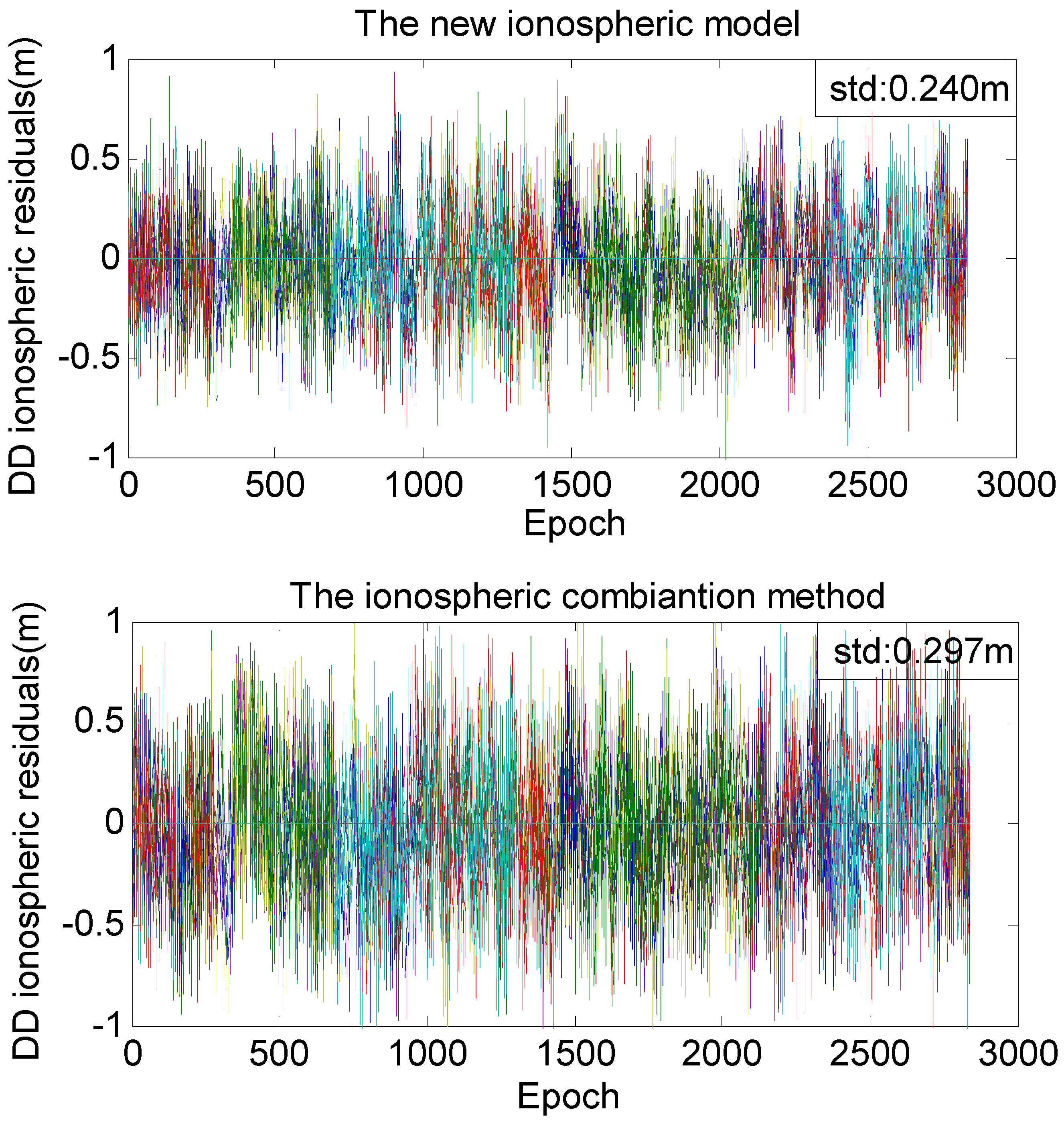
Section 4.1). Compared with the ionospheric combination method, which performs ionospheric estimates at a precision level of 0.3 m [22], the new ionospheric model has more degrees of freedom. Additionally, model estimates have been instantaneously smoothed by the epoch-differenced ionospheric information with high precision (refer to Section 4.2). Thus, the precision of real-time ionospheric estimates is expected to be better than 0.1 m. Second, ionospheric estimations with high precision are added into the geometry-based model, extending the geometry-related model into an ionosphere-weighted model (refer to Section 4.3). Ionospheric constraints can help to enhance the strength of the observation model and thereby reduce convergence time of unknowns, especially the ionospheric unknown. These modifications help to shorten the time to TFFS compared to the current observation model without any constraints.
It is known that EWL ambiguity can be reliably determined in a single epoch. Even for long baselines with hundreds of kilometres, the success rate of the current EWL AR can reach 99%. The EWL resolution in the new method also refers to Equations (2) and (3). We then used Equation (4) to resolve the WL ambiguities.

4.1. New Model of Estimating DD Ionospheric Delay

Before the DD ionospheric model is formulated, the following independent variables exist: three pseudorange observations, three phase observations, two EWL ambiguities and two WL ambiguities. To increase the degrees of freedom in the model and avoid singularities, only eight variables can be selected, and the corresponding general model can be used to calculate the ionospheric delay, expressed as follows:
D D i o n ( x i ( i = 1 , .. , 8 ) ) = x 1 ϕ ( 1 , 0 , 0 ) + x 2 ϕ ( 0 , 1 , 0 ) + x 3 ϕ ( 0 , 0 , 1 ) + x 5 p ( 1 , 0 , 0 ) + x 6 p ( 0 , 1 , 0 ) + x 7 p ( 0 , 0 , 1 ) + x 8 N ( 1 , 0 , 1 )
To optimize the model, Equation (7) should obey the following constraints:
  • Geometry-free condition:
    x 1 + x 2 + x 3 + x 4 + x 5 + x 6 = 0
  • Retain the remaining DD ionosphere delay:
    x 1 η ( 1 , 0 , 0 ) x 2 η ( 0 , 1 , 0 ) x 3 η ( 0 , 0 , 1 ) + x 4 η ( 1 , 0 , 0 ) + x 5 η ( 0 , 1 , 0 ) + x 6 η ( 0 , 0 , 1 ) = 1
  • Eliminate N(1,0,0):
    x 1 λ ( 1 , 0 , 0 ) + x 7 + x 8 = 0
  • Eliminate N(0,1,0):
    x 2 λ ( 0 , 1 , 0 ) x 7 = 0
  • Eliminate N(0,0,1):
    x 3 λ ( 0 , 0 , 1 ) x 8 = 0
  • Minimize the noise condition:
    ( x 1 2 + x 2 2 + x 3 2 ) σ p 2 + ( x 4 2 + x 5 2 + x 6 2 ) σ ϕ 2 = min
The pseudorange and phase observables are correlated with each other by shared errors. However, the correlations are eliminated and do not contribute to the minimum noise condition due to geometry-free constraints; a detailed deduction process is outlined by Vollath and Sauer [23]. Based on this, the ratio of pseudorange and phase noise is important in minimizing the noise condition, and it directly affects estimation of the unknowns. 
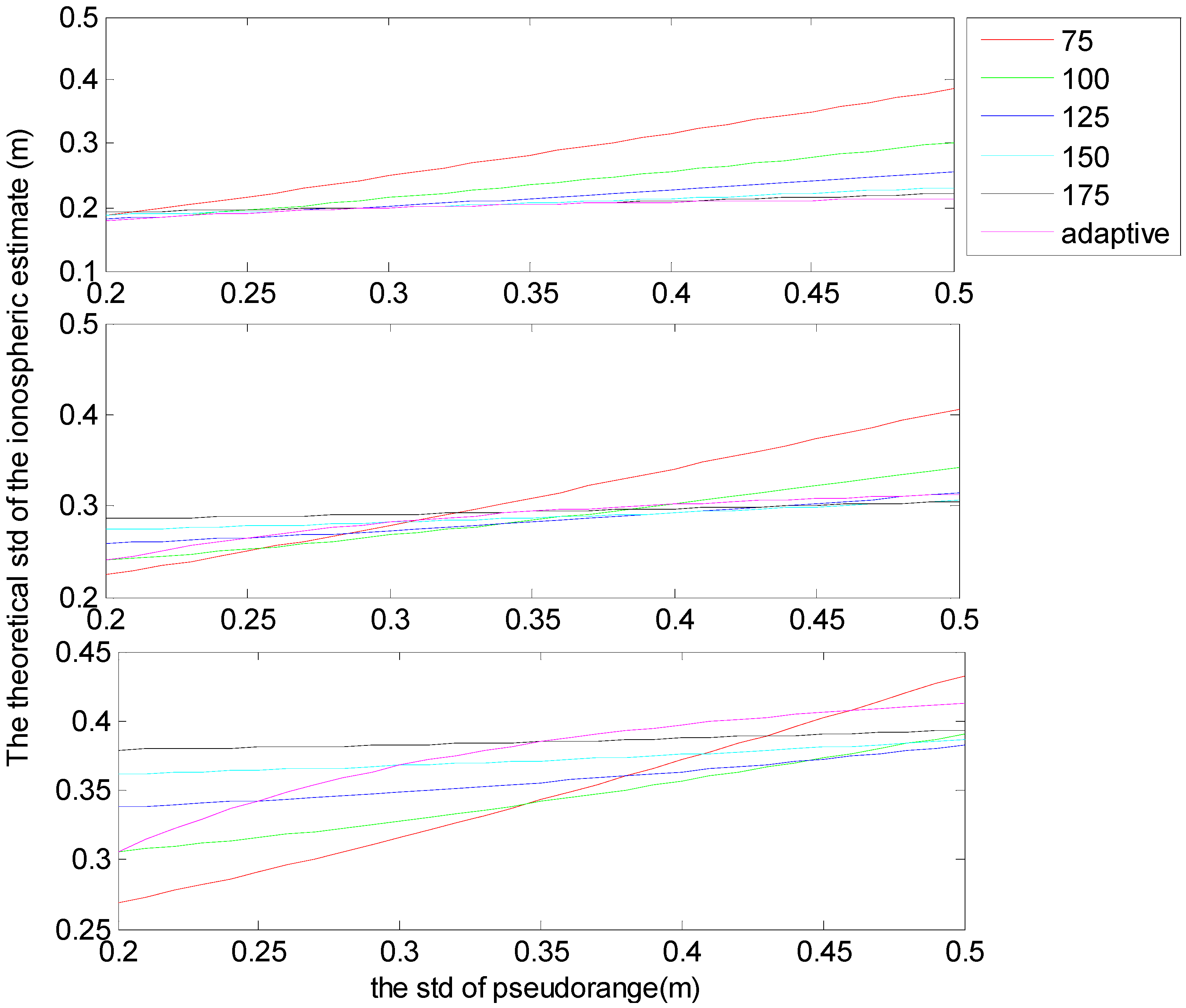
Figure 1 illustrates correlations between theoretical standard deviations of optimal DD ionospheric estimations and phase noise, as well as correlations between standard deviations of ionospheric estimations and pseudorange noise. Although the ratio of pseudorange and phase noise may occasionally vary, estimates using 125 as the ratio are the closest to that from the adaptive estimates, and the deviations are smaller than when the ratio is 75, 100, 125 and 150. Based on the above deductions and to enable straightforward computation, we set the ratio to 125; estimations of the unknowns from Equation (7) are summarized in Table 2.
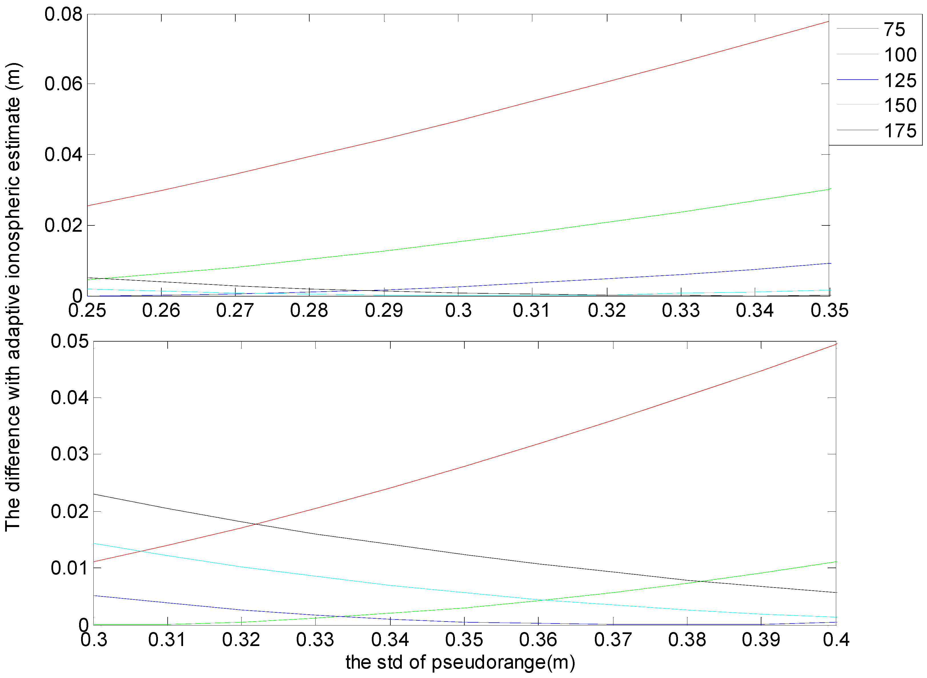
As we all know, the standard deviation (std) of phase observables mainly range from 0.2 mm to 0.3 mm. When the phase noise is around 0.3 mm, the corresponding std of pseudorange observable often limits from 0.3 m to 0.4 m. For the above-mentioned conditions, Figure 2 presents the corresponding differences between ionospheric estimates and adaptive estimates. It can be seen from Figure 2, the estimates from the ratio of 125 is almost the closest to that from the adaptive estimates. Although there are two exceptions: in the top panel, when pseudorange noise ranges from 0.3 m to 0.35 m, the difference between ionospheric estimated from the ratio of 125 is larger than that from the ratio of 150; and, in the bottom panel, when pseudorange noise range from 0.3 m to 0.35 m, the difference between ionospheric estimated from the ratio of 125 is larger than that from the ratio of 100. However, for these two exceptional conditions, the maximum difference is only 0.7 mm, which happens at the top panel when the pseudorange is 0.35 m. Thus, the deviation is not obvious, and the ionospheric estimates from ratio of 125 is still can be believed has the optimum performance.

4.2. Smoothed Ionospheric Delay Estimates

We can obtain epoch-differenced ionospheric information with high precision by using the following equations:
I o n ( k ) = ϕ ( 1 , 0 , 0 ) ( k ) ϕ ( 0 , 1 , 0 ) ( k ) η ( 1 , 0 , 0 ) η ( 0 , 1 , 0 ) λ ( 1 , 0 , 0 ) N ( 1 , 0 , 0 ) λ ( 0 , 1 , 0 ) N ( 0 , 1 , 0 ) η ( 1 , 0 , 0 ) η ( 0 , 1 , 0 )
Δ I o n ( k 1 , k ) = ( ϕ ( 1 , 0 , 0 ) ( k ) ϕ ( 1 , 0 , 0 ) ( k 1 ) ) ( ϕ ( 0 , 1 , 0 ) ( k ) ϕ ( 0 , 1 , 0 ) ( k 1 ) ) η ( 1 , 0 , 0 ) η ( 0 , 1 , 0 )
where the symbol k represents the current epoch. After ionosphere has been determined, we use Equation (10) to obtain more precise DD ionospheric estimates.
I o n ~ ( k ) = ω D D i o n ( k ) + ( 1 ω ) ( I o n ~ ( k 1 ) + Δ I o n ( k 1 , k ) )
In Equation (10), weighting factor equals to inversion of the smoothing length.
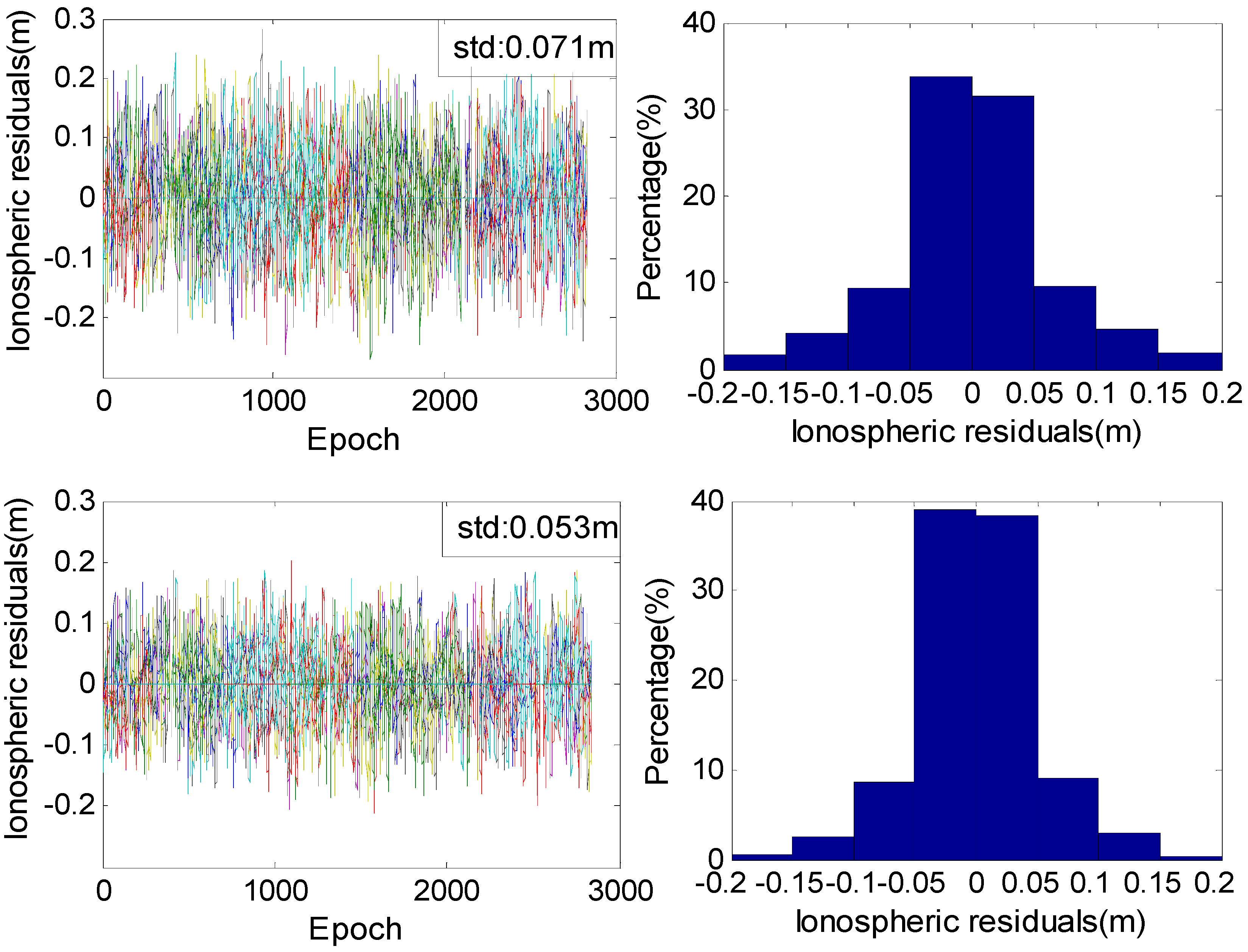
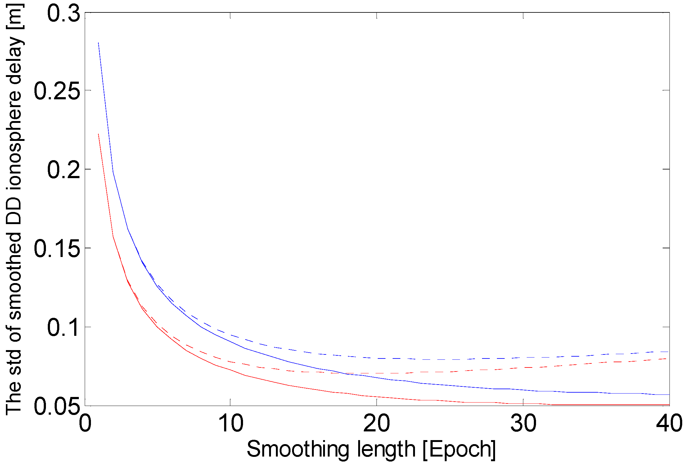
Considering higher-order ionosphere effects and combination noise, the standard deviation of ionosphere will generally range from 0.01 to 0.02 m [24,25]. In Figure 3, given the same smoothing length, the precision of ionospheric delay estimates from the new method is always better than that from the current ionospheric combination method. When the standard deviation of ionospheric is 0.02 m, the precision of ionospheric from the new method initially improves as the smoothing length increases, reaching an optimal smoothing length at 16 epochs, and then the standard deviation increases as the length increases. If ionospheric has a standard deviation of 0.01 m, the new method obtains ionospheric with nearly the same standard deviation when the smoothing length is equal to or more than 16 epochs. With the new method, when Equation (10) is used to estimate ionospheric, the smoothing window should updates instantaneously, and the maximum smoothing length could be set to 16 epochs.
In Equation (10), if the two WL ambiguities are not correctly determined, the ionospheric estimates from Equation (7) will be seriously deteriorated, which thus affects the current estimate and the 15 subsequent epochs’ ionospheric estimates from Equation (10). Although this phenomenon is rare, we use the following test to avoid it:
| D D i o n ( t ) ( I o n ( k 1 ) + Δ I o n ~ ( k 1 , k ) ) | < γ
where adaptive value is an empirical value set to 1.0. Table 2 suggests that wrongly determined WL ambiguities will cause a systematic bias in ionosphere of at least 2. In addition, Figure 3 shows that the standard deviation of adaptive value is slightly smaller than 0.4 and that the double values of the standard deviation of adaptive value is only 0.8. Based on the two deductions, setting adaptive value to 1.0 can distinguish whether the WL ambiguities are wrong fixed or not. If the test fails, one could use the results derived from Equation (12) as the optimal ionospheric estimate for the current epoch.
I o n ~ ( t ) = I o n ~ ( t - 1 ) + Δ I o n ( t 1 , t )

4.3. NL Ambiguity Resolution

To transform DD ionospheric estimates from Step 2 into ionospheric constraints, derived ionospheric estimates are employed as pseudoranges and assimilated into the current observation model. After this step, Equation (5) can be extended as follows:
[ v E W L v W L v 1 v I o n ] = [ B 0 I τ I η ( 0 , 1 , 1 ) B 0 I τ I η ( 1 , 1 , 0 ) B I λ ( 1 , 0 , 0 ) I τ I η ( 1 , 1 , 0 ) B 0 I τ I ] [ Δ X N ( 1 , 0 , 0 ) t r o I o n ] [ l E W L l W L l 1 l I o n ]
where the parameters at the left of the equation represents the difference between the ionospheric delay estimate and the actual delay In the filtering process, the covariance between ionospheric delay estimate and other observables (or combinations) can be computed by the error propagation law. In addition, the variance of its own is conservatively set as follows:
s t d = { 0.2 m t < δ 1 0.1 m δ 1 < t < δ 2 0.08 m δ 2 < t < δ 3 0.06 m t = δ 3
where three adaptive value are set to 5, 10 and 16, respectively. The values in Equation (14) are determined according to 
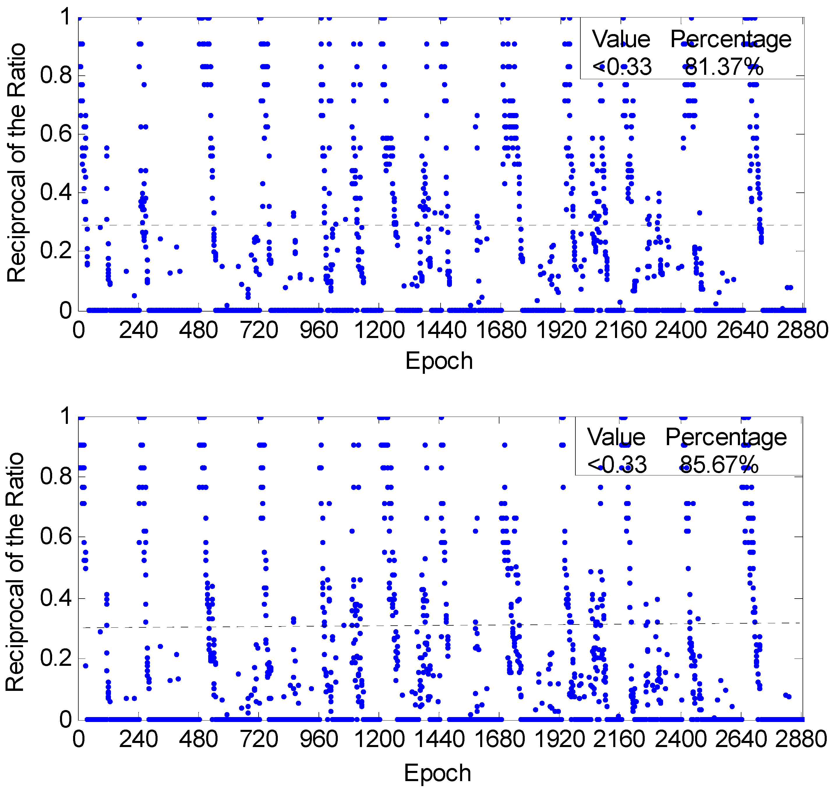
Figure 3, and they will be further evaluated in later experiments to confirm proper value settings. We used the LAMBDA algorithm to search and fix ambiguities, and the epoch is identified as fixed when the ratio is larger than 3. Ratio is estimated by using Equation (15):
a a 2 Q a 2 a a 1 Q a 2 = R 2 R 1 C
where Equation (15) is used for the squared norm of ambiguity residuals of the best, and second-best integer solution, respectively, as measured by the squared norm of the ambiguity residual vector. C is the discriminative value, a fixed value is used in many software package, e.g., 3, which is also the same in our experiments.
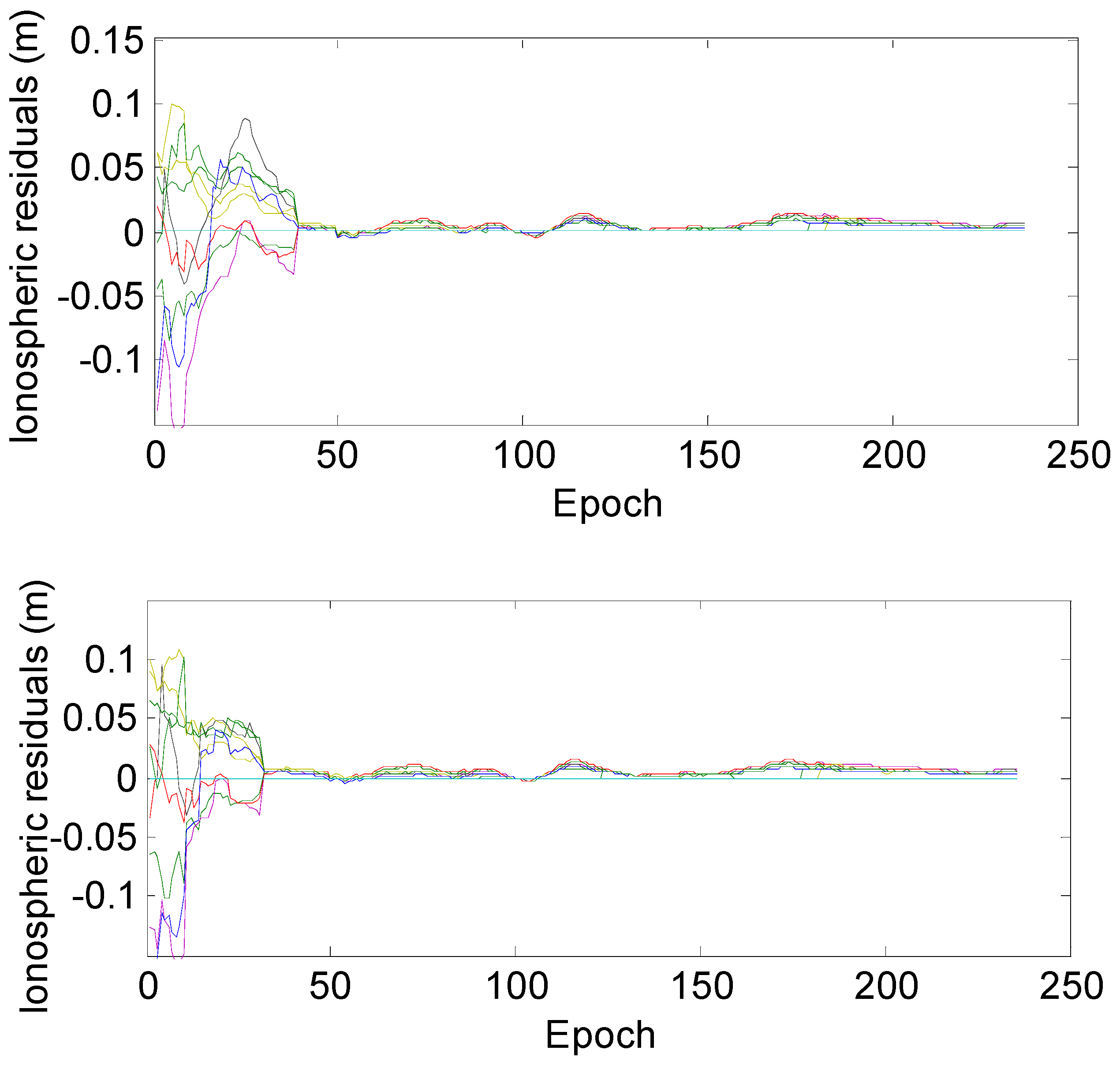
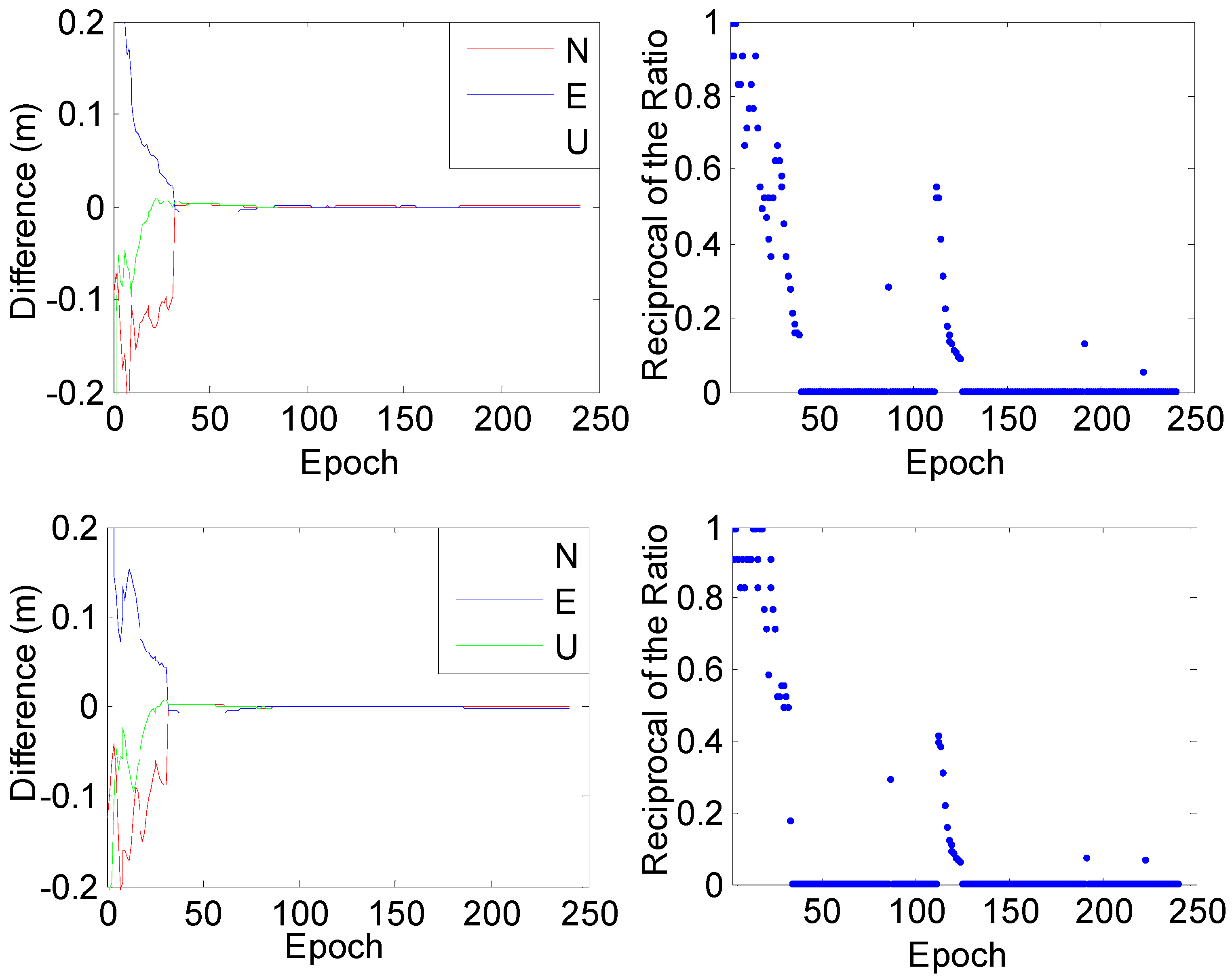
These ionospheric estimates may enhance the strength of the current model and thereby shorten the convergence time of the unknowns. This assumption will also be verified in subsequent tests using actual observational data.

5. Experiments and Analysis

To demonstrate the new TCAR and evaluate its performance, we selected three independent long baselines (HOFN-MYVA, OBE4-WTZ3 and LLAG-MASL) with distances longer than 100 km as the experiment conditions. The corresponding HOFN-MYVA, OBE4-WTZ3 and LLAG-MASL baseline lengths are 173 km, 166 km and 104 km, respectively. Six GNSS stations (HOFN, MYVA, OBE4, WTZ3, LLAG and MASL) belonging to the MGEX network were arbitrarily chosen. The experimental GPS observations were collected from 21 to 30 January 2015 with a sampling interval of 30 s. When there were only two frequency signals recorded in the raw file, the semi-generated method was used to simulate the third frequency signal. Here, for simplicity, we show only the results from the baseline of HOFN-MYVA on 21 January 2015 to compare the performance of our new method and the current method. The results at other baselines for the two methods are similar.

5.1. Evaluate the Precision of the Ionospheric Estimates

Figure 4 shows DD ionospheric estimates using the post-processing method. It can be observed that the ionospheric exhibits large daily variations, and its effect cannot be eliminated by double differencing operation.
Figure 5 demonstrates the performances of the two ionospheric models. The standard deviation of the ionospheric delays estimated from the new method is 20% less than that from the combination method.
Figure 6 shows the standard deviations of ionospheric delays derived from smoothing lengths of 10 and 16 epochs. The standard deviation of ionospheric estimations can be less than 0.08 m when the smoothing length is 10 epochs; it decreases to 0.06 m when the smoothing length is increased to 16 epochs. These results about precision versus smoothing length agree well with the deductions shown in Figure 3 and the values calculated with Equation (14). When the smoothing length is 16 epochs, the smoothed ionospheric estimates can achieve magnitudes defined to the nearest centimetre, which creates a favourable condition to shorten the convergence time for the unknown parameters.

5.2. Evaluate the Performance of NL Resolution

To differentiate it from the new method, the current TCAR method, introduced in Section 2, is hereafter referred to as the old method. We divide the daily GPS data on Day 21 of the year (Doy) into 12 non-overlapping portions. Each portion contains two hours of data and has been, respectively, processed by the new and old methods. We use the TFFS and positioning experiments to evaluate the AR performance [26,27,28,29,30]. In the positioning experiments, we take station HOFN as base station; its precise coordinate comes from weekly solutions. We take station MYVA as the rover station; the positioning errors can be computed by subtracting the estimated coordinates from the precisely observed ground coordinates.
Figure 7 and Figure 8 illustrate the results from the first part of the experiments. The ionospheric residuals will dramatically decreased as the ambiguity is fixed. The two figures consistently show that the TFFS with the old method is 39 epochs, decreasing to 32 epochs with the new method. For the ionospheric estimations derived from the new method (bottom panel), the differences between DD ionospheric delay estimations and actual values are generally less than 0.05 m after the 16th epoch, and their magnitudes are smaller than those estimated from the old method (top panel).
Table 3 summarizes the TFFS for all 12 portions. Using the old method, the TFFS ranges from 20 to 25 min; with the new method, the TFFS decreases to 15 to 20 min. The average TFFS for the new method is 20% less than the old method. The TFFS of the three baselines are shown in Figure 9.
T1 and T2, respectively, represent the TFFS for the old and the new method, I represents the improvement, and the calculation process is as follows:
I = T 1 T 2 T 1 100 %
As shown in Table 3, using the new method, the IAR successfully finished within 30 min for all 12 experimental cases. Thus, Figure 10 explicitly describes ionospheric estimates in only the first 60 epochs for each case. It can be observed that the ionospheric residuals from the 16th epoch are nearly within 0 to 5 cm for the new method and that its magnitude is clearly smaller than that from the old method. It should also be noted that after the ambiguities have been successfully determined, the ionospheric variations estimated from the two methods are similar. A possible reason for this finding could be that the precision of the ionospheric delay estimates obtained through filtering are much better than those from the ionospheric model; thus, the ionospheric constraints contribute little. In addition, the variations of ionospheric estimates from both methods show the same error pattern after successful IAR. Figure 7 supports this conclusion. The errors are systematic, and the source is uncorrected model errors. Even though these errors may cause a maximum bias of nearly 3 cm (Figure 10), the error magnitude is only 15% of the magnitude of the wavelength; as such, it can be considered negligible for the IAR.
Figure 11 reflects the overall ambiguity estimations with the reciprocals of the ratio results. The reciprocal results, which are less than 0.33 from the new method, are 4.3% more than those from the old method. These results indicate that the TFFS with ionospheric constraints can save 10 epochs equally by comparing with the results without using the ionospheric constraints in each experimental case, which further verify that the ionospheric constraints are helpful to the IAR.
New proposed method is also applied in the baselines of BJF1-BJXT, SHA1-ZJKD, WUH1-HBF2 and CHA1-CHSW. Their baseline length and TFFS are summarized in Table 4.
Derived from Table 4, our method has the optimum performance when the baseline length is around 166 km. When the length of baseline is longer than 166 km, with the baseline length increases, the improvement of TFFS derived from our new method will decrease from 26% to 13%. When the baseline length is shorter than 166 km, the improvement of TFFS derived from our method will increase from 10% to 26%. When the baseline length is shorter than 100 km, the double-differenced operation will help to eliminate some shared errors, thus the TFFS will be limited to around 20 min if only use the common geometry-based method, our method des not seem to contribute too much under this condition. When the baseline length is longer than 200 km, the ambiguity resolution is easily affected by some un-modelled (or not correctly modelled) errors. Under this condition, our method seems help less than this case when the baseline length is shorter than 200 km.

6. Summary

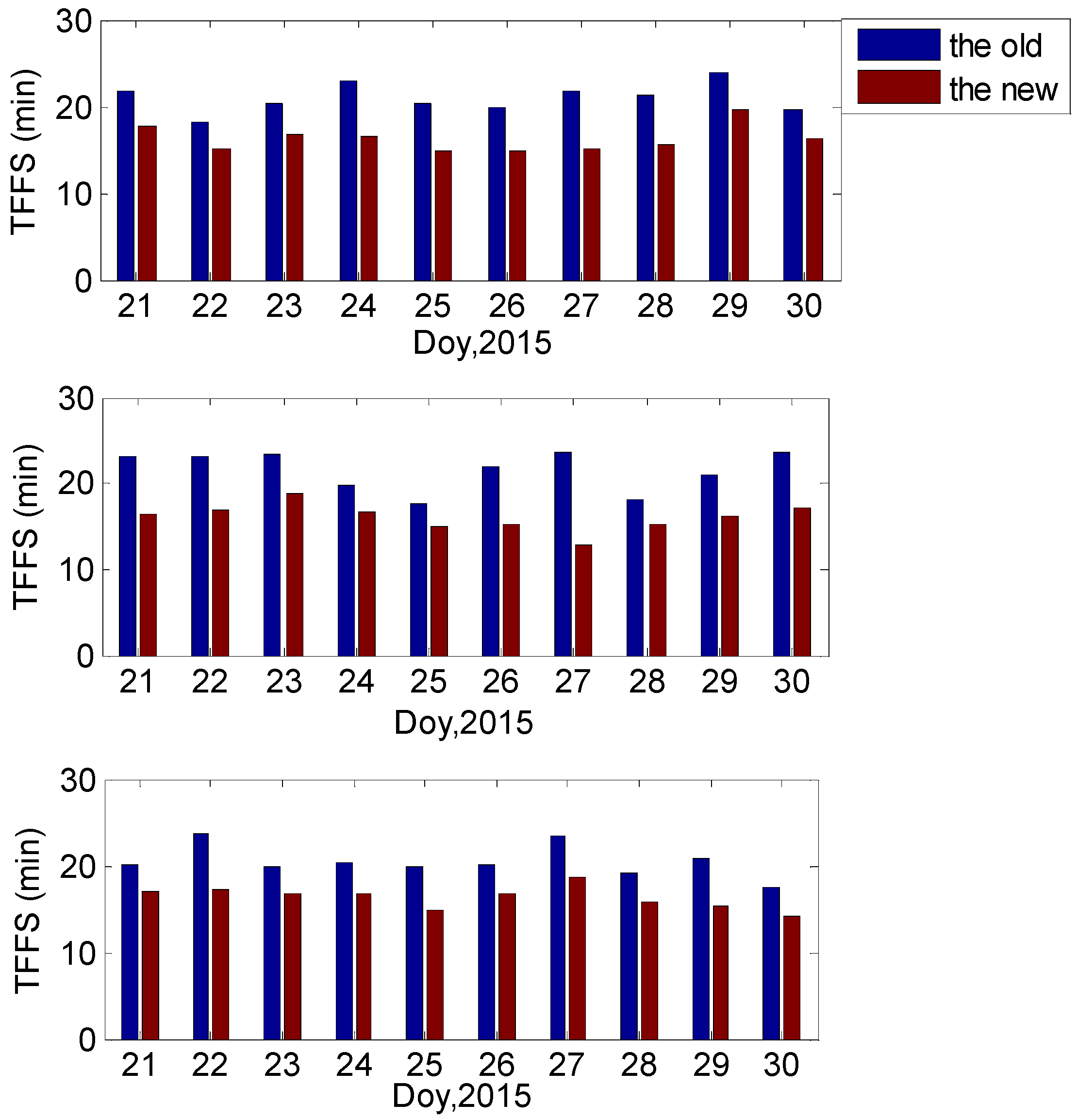
Being affected by DD ionospheric residuals, the current TCARs need to accumulate long periods of data for successful IAR. Current IAR algorithms generally take 20 to 25 min, which is a little long for fast positioning. To shorten the IAR time, we propose a new TCAR algorithm by adding realistic ionospheric information constraints. We modified the current TCAR methods in three aspects. First, a new ionospheric model is developed to estimate the DD ionospheric delay. Compared to previous combination methods, the original pseudorange and phase observations are introduced to increase the degrees of freedom and minimize noise constraints. In doing so, the ionospheric delay estimates are globally optimized. Both theoretical derivations and the experimental results indicate that the precision of the ionospheric delay estimated from our new model is 20% higher than that from the current ionospheric combination method. Second, the epoch-differenced ionospheric information is used to smooth the ionospheric delay by employing the Hatch algorithm. Using theoretical derivations and sensitivity tests, we found that the most suitable smoothing length is 16 epochs and that the smoothed ionospheric delay could reach a magnitude of precision defined to the nearest centimetre. For cases in which wrongly determined WL ambiguities deteriorate the precision of smoothed ionospheric delay estimations, we also proposed a set of error diagnosis and resolutions. Third, the smoothed ionospheric delays obtained from Step 2 are treated as pseudorange observable values and are added to the original model to strengthen the original observation equation, thus extending the current geometry-based model into an ionosphere-weighted model. The results show that this model can improve the convergence efficiency of the unknowns, especially the ionospheric unknown. The model creates favourable conditions for fast and successful IAR. After the above three modifications, the new formulated TCAR algorithm reduces the IAR convergence time by 20% compared to the current TCAR method. If we use the new ionospheric model to estimate ionospheric delay before the filtering process, the convergence time is expected to be shorter.
In summary, we investigated, theoretically and practically, the feasibility of employing a new ionospheric model as constraints to speed up the IAR. The direct benefit is that the new model reduces IAR time by 20% compared to the current TCAR method. Additionally, it provides precise information to further investigate long-baseline relative positioning, especially for the Beidou system, which features triple-frequency data on all satellites. The ionospheric delay used in the constraints is provided in real time by our method, acting as an optional way of assisting real-time relative positioning. We also provide a new strategy for estimating DD ionospheric delay with a precision to the nearest centimetre, which is expected to be helpful for directly studying the ionosphere.

Acknowledgments

Thanks are given for the constructive comments from the three anonymous reviewers. This work was partially supported by National key Research Program of China “Collaborative Precision Positioning Project” (No. 2016YFB0501900), the National Nature Science Foundation of China (No. 41231064, 41674022, 41304034, 41574032 and 41304033). We also acknowledge the funding support provided by the State Key Laboratory of Geodesy and Earth’s Dynamics (Institute of Geodesy and Geophysics, CAS) (No. SKLGED2014-3-1-E).

Author Contributions

Yafei Ning and Yunbin Yuan provided the initial idea for this study; Yafei Ning and Yanju Chai conceived and designed the experiments; Yafei Ning and Bingfeng Tan analysed the experiment results; and Yafei Ning and Zhen Huang wrote the paper.

Conflicts of Interest

The authors declare no conflict of interest.

References

  1. Li, B.; Shen, Y.; Feng, Y. Long-range real-time precise navigation with three frequency GNSS. Geomat. Inf. Sci. Wuhan Univ. 2009, 34, 782–786. [Google Scholar]
  2. Zhao, Q.; Dai, Z.; Hu, Z.; Sun, B.; Shi, C.; Liu, J. Three-carrier ambiguity resolution using the modified TCAR method. GPS Solut. 2015, 19, 589–599. [Google Scholar] [CrossRef]
  3. Gao, W.; Gao, C.; Pan, S. Single-epoch positioning method in network RTK with BDS triple-frequency wide lane combinations. J. Navig. 2016, 69, 1293–1309. [Google Scholar] [CrossRef]
  4. Feng, Y.; Rizos, C. Three carrier approaches for future global, regional and local GNSS positioning services: Concepts and performance perspectives. In Proceedings of the ION GNSS 2005, Tampa, FL, USA, 14–18 September 2005.
  5. Ji, S. Positioning Performance Improvements with European Multiple-Frequency Satellite Navigation System-Galileo. Ph.D. Thesis, Hong Kong Polytechnic University, Hong Kong, China, 2008. [Google Scholar]
  6. Zhang, W.; Cannon, M.E.; Julien, O.; Alves, P. Investigation of combined GPS/Galileo cascading ambiguity resolution schemes. In Proceedings of the ION GPS/GNSS 2003, Portland, OR, USA, 9–12 September 2003.
  7. Vollath, U. The factorized multi-carrier ambiguity resolution (FAMCAR) approach for efficient carrier-phase ambiguity estimation. In Proceedings of the ION GNSS 2004, Long Beach, CA, USA, 21–24 September 2004.
  8. Feng, Y. GNSS three carrier ambiguity resolution using ionosphere-reduced virtual signals. J. Geod. 2008, 82, 847–862. [Google Scholar] [CrossRef]
  9. Hatch, R. A new three-frequency, geometry-free technique for ambiguity resolution. In Proceedings of the ION GPS/GNSS 2006, Fort Worth, TX, USA, 26–29 September 2006.
  10. Li, X.; Ge, M.; Dai, X.; Ren, X.; Fritsche, M.; Wickert, J.; Schuh, H. Accuracy and reliability of multi-GNSS real-time precise positioning: GPS, GLONASS, BeiDou, and Galileo. J. Geod. 2015, 89, 607–635. [Google Scholar] [CrossRef]
  11. Li, X.; Ge, M.; Zhang, H.; Nischan, T.; Wickert, J. The GFZ real-time GNSS precise positioning service system and its adaption for compass. Adv. Space Res. 2013, 51, 1008–1018. [Google Scholar] [CrossRef]
  12. Li, X.; Zus, F.; Lu, C.; Dick, G.; Ning, T.; Ge, M.; Wickert, J.; Schuh, H. Retrieving of atmospheric parameters from multi-GNSS in real time: Validation with water vapor radiometer and numerical weather model. J. Geophys. Res. Atmos. 2015, 120, 7189–7204. [Google Scholar] [CrossRef]
  13. Xu, Y.; Ji, S.; Chen, W.; Weng, D. A new ionosphere-free ambiguity resolution method for long-range baseline with GNSS triple-frequency signals. Adv. Space Res. 2015, 56, 1600–1612. [Google Scholar] [CrossRef]
  14. Tang, W.; Deng, C.; Shi, C.; Liu, J. Triple-frequency carrier ambiguity resolution for BeiDou navigation satellite system. GPS Solut. 2014, 18, 335–344. [Google Scholar] [CrossRef]
  15. Odijk, D. Weighting ionospheric corrections to improve fast GPS positioning over medium distances. In Proceedings of the ION GPS 2000, Salt Lake City, UT, USA, 19–22 September 2000.
  16. Yuan, Y. Study on Theories and Methods of Correcting Ionospheric Delay and Monitoring Ionosphere Baseon GPS. Ph.D. Thesis, Institute of Geodesy and Geophysics Chinese Academy of Sciences, Wuhan, China, 2002. [Google Scholar]
  17. Li, B.; Shen, Y.; Zhou, Z. A new method for medium and long range three frequency GNSS rapid ambiguity resolution. Acta Geod. Cartogr. Sin. 2009, 38, 296–301. [Google Scholar]
  18. Teunissen, P.J. A new method for fast carrier phase ambiguity estimation. In Proceedings of the Position Location and Navigation Symposium 1994, Las Vegas, NV, USA, 11–15 September 1994.
  19. Teunissen, P.J. The least-squares ambiguity decorrelation adjustment: A method for fast GPS integer ambiguity estimation. J. Geod. 1995, 70, 65–82. [Google Scholar] [CrossRef]
  20. Teunissen, P.J. An optimality property of the integer least-squares estimator. J. Geod. 1999, 73, 587–593. [Google Scholar] [CrossRef]
  21. Verhagen, S.; Li, B.; Teunissen, P.J. Ps-lambda: Ambiguity success rate evaluation software for interferometric applications. Comput. Geosci. 2013, 54, 361–376. [Google Scholar] [CrossRef]
  22. Li, B.; Feng, Y.; Shen, Y. Three carrier ambiguity resolution: Distance-independent performance demonstrated using semi-generated triple frequency GPS signals. GPS Solut. 2010, 14, 177–184. [Google Scholar] [CrossRef]
  23. Vollath, U.; Sauer, K. Famcar approach for efficient multi-carrier ambiguity estimation. In Proceedings of the ENC-GNSS 2004, Rotterdam, The Netherlands, 16–19 May 2004.
  24. Yuan, Y.; Huo, X.; Ou, J. Models and methods for precise determination of ionospheric delay using GPS. Prog. Nat. Sci. 2007, 17, 187–196. [Google Scholar]
  25. Yuan, Y.; Ou, J. An improvement to ionospheric delay correction for single-frequency GPS users—The APR-I scheme. J. Geod. 2001, 75, 331–336. [Google Scholar] [CrossRef]
  26. Zhang, B.; Ou, J.; Yuan, Y.; Zhong, S. Yaw attitude of eclipsing GPS satellites and its impact on solutions from precise point positioning. Chin. Sci. Bull. 2010, 55, 3687–3693. [Google Scholar] [CrossRef]
  27. Zhang, B.; Teunissen, P. Zero-baseline analysis of GPS/BeiDou/Galileo between-receiver differential code biases (BR-DCBS): Time-wise retrieval and preliminary characterization. Navigation 2016. [Google Scholar] [CrossRef]
  28. Zhang, B. Three methods to retrieve slant total electron content measurements from ground-based GPS receivers and performance assessment. Radio Sci. 2016, 51, 972–988. [Google Scholar] [CrossRef]
  29. Zhang, B.; Yuan, Y.; Chai, Y. QIF-based GPS long-baseline ambiguity resolution with the aid of atmospheric delays determined by PPP. J. Navig. 2016. [Google Scholar] [CrossRef]
  30. Tan, B.; Yuan, Y.; Zhang, B.; Hsu, H.Z.; Ou, J. A new analytical solar radiation pressure model for current BeiDou satellites: IGGBSPM. Sci. Rep. 2016. [Google Scholar] [CrossRef] [PubMed]
Figure 1. The theoretical standard deviations (std) of the DD ionospheric delay estimates versus the std of the pseudorange observations; the std of the phase observation is 2 mm (top); 3 mm (middle) and 4 mm (bottom). “Adaptive” represents the estimation where the ratio satisfies the real value, and the other lines with different colours represent estimations when the ratios are constants (75, 100, 125, 150, and 175).
Ijgi 05 00198 g001
Figure 2. The differences between theoretical std of the DD ionospheric delay estimates and the adaptive estimates; the std of the phase observation is, respectively, 2 mm (top) and 3 mm (bottom). The “adaptive” represents the estimation with the ratio is satisfied with the real one, and the other lines with different colours represent the estimations when the ratios are constants (75, 100, 125, 150, and 175).
Ijgi 05 00198 g002
Figure 3. The theoretical standard deviation (std) of ionospheric versus the smoothing length. Blue indicates the results when the std of ionospheric is 0.02 m, red indicate the results when the std of ionospheric is 0.01 m, solid lines represent the results from the new ionospheric model, and dashed lines represent the estimates of ionospheric delay derived from the combination method.
Ijgi 05 00198 g003
Figure 4. The DD ionospheric delay over HOFN-MYVA baseline on 21 January 2015.
Ijgi 05 00198 g004
Figure 5. Differences between ionospheric estimates and actual values as estimated by the new ionospheric model (top) and the combination method (bottom).
Ijgi 05 00198 g005
Figure 6. Differences between smoothed ionospheric delay estimates and the actual values when the smoothing length is 10 (top) and 16 (bottom) epochs. Detailed distributions are depicted on the right.
Ijgi 05 00198 g006
Figure 7. Ionospheric residuals derived by the old method (top) and the new method (bottom) for the first portion.
Ijgi 05 00198 g007
Figure 8. Positioning results with the old method (top) and the new method (bottom) for the first portion; the reciprocals of their ratio values are described on the right.
Ijgi 05 00198 g008
Figure 9. Average TFFS on the baselines of HOFN-MYVA (top); OBE4-WTZ3 (middle) and LLAG-MASL (bottom).
Ijgi 05 00198 g009
Figure 10. Ionospheric residuals estimated by the old (top) and the new (bottom) methods during the first 60 epochs for the 12 cases.
Ijgi 05 00198 g010
Figure 11. Reciprocals of the ratios of the 12 portions; they are, respectively derived by the old (top) and the new (bottom) methods. The annotation 1 indicates that ratio = 1, the annotation 0 corresponds to fixed epochs, and the dash indicates that the ratio is 3.
Ijgi 05 00198 g011
Table 1. The wavelength, ionospheric scalar factor and noise amplitude factor for the NL/WL/EWL combinations.
Class ϕ ( i , j , k ) λ ( i , j , k ) η ( i , j , k ) μ ( i , j , k )
NL ϕ ( 1 , 0 , 0 ) 0.19011
ϕ ( 0 , 1 , 0 ) 0.2441.6471
ϕ ( 0 , 0 , 1 ) 0.2551.7931
WL ϕ ( 1 , 0 , 1 ) 0.751−1.3394.930
ϕ ( 1 , 1 , 0 ) 0.862−1.2835.740
EWL ϕ ( 1 , 6 , 5 ) 3.256−0.0744103.80
ϕ ( 0 , 1 , 1 ) 5.861−1.71933.24
Table 2. Estimated coefficients in Equation (7).
x1x2x3x4x5x6x7x8
−12.4668.29−56.07−0.140.150.21−16.6614.30
Table 3. The TFFS in the 12 portions on the HOFN-MYVA baseline.
Observation Time SpanT1
(Epoch)
T2
(Epoch)
I
(%)
1393217.95
2363016.67
3503922.00
4342526.47
516156.25
6615116.39
7272218.52
8715325.35
9392925.64
10483722.92
11403025.00
12655023.08
Mean43.7634.3421.53
Table 4. The TFFS results derived from different baseline lengths.
Baseline NameBaseline Length (km)T1 (min)T2 (min)I (%)
BJF1-BJXT7820.6717.0117.71
LLAG-MASL10421.4217.3019.23
OBE4-MTZ316625.7118.9926.14
HOFN-MYVA17323.3919.6116.16
SHA1-ZJKD20728.5022.4221.33
WUH1-HBF224427.8223.6415.03
CHA1-CHSW25828.9525.0713.40

