Article

Morphological PDEs on Graphs for Image Processing on Surfaces and Point Clouds

by
Abderrahim Elmoataz
1,2,*,
François Lozes
2 and
Hugues Talbot
1
1
A3SI Team, University of Paris-Est Marne-La-Vallée int the LIGIM Laboratory, Cité Descartes, Bâtiment Copernic-5, Boulevard Descartes, Champs sur Marne, 77454 Marne-la-Vallée Cedex 2, France
2
Image Team, University of Caen Normandy and the ENSICAEN in the GREYC Laboratory, 6 Boulevard Maréchal Juin, F-14050 Caen Cedex, France
*
Author to whom correspondence should be addressed.
ISPRS Int. J. Geo-Inf. 2016, 5(11), 213; https://0-doi-org.brum.beds.ac.uk/10.3390/ijgi5110213
Submission received: 30 June 2016 / Revised: 24 October 2016 / Accepted: 4 November 2016 / Published: 12 November 2016
(This article belongs to the Special Issue Mathematical Morphology in Geoinformatics)

Abstract

:
Partial Differential Equations (PDEs)-based morphology offers a wide range of continuous operators to address various image processing problems. Most of these operators are formulated as Hamilton–Jacobi equations or curve evolution level set and morphological flows. In our previous works, we have proposed a simple method to solve PDEs on point clouds using the framework of PdEs (Partial difference Equations) on graphs. In this paper, we propose to apply a large class of morphological-based operators on graphs for processing raw 3D point clouds and extend their applications for the processing of colored point clouds of geo-informatics 3D data. Through illustrations, we show that this simple framework can be used in the resolution of many applications for geo-informatics purposes.

1. Introduction

Partial Differential Equations (PDEs) are widely used for modeling and solving many inverse problems in image processing and computer vision. PDEs of the Laplacian or p-Laplacian type have been used successfully in many applications, such as image denoising, restoration, segmentation and inpainting; see [1,2,3,4] and the references therein. PDEs of the Hamilton–Jacobi type play a central role in continuous mathematical morphology. They have been used to model many continuous morphological operators, such as dilation, erosion, leveling or watershed transforms [5,6,7,8,9]. However, many of these models focus on images defined on the Euclidean domain where discretization, based on finite differences, finite elements, finite volumes, etc, is well investigated and traditionally used.
On the other hand, with the development of 3D scanning technology, it is now easy to generate 3D models from real objects, together with standard images painted on them. LIDAR (Light Detection and Ranging) scanners allow one to generate point clouds by estimating the distance between sensors and ground objects and have found interest in geoscience; see [10,11,12,13]. These scanners generally provide raw data in the form of (noisy) unorganized point clouds representing surface samples with images on point clouds. With the increasing popularity and the very broad applications in geoscience, art, medicine and security of manufacturing, there is a growing interest to transpose PDEs-based tools for signal/image processing to image processing on point clouds. The discretization of differential operators becomes more difficult compared to the previously mentioned approaches.
There are a variety of methods for solving PDEs on surfaces numerically [14,15,16]. However, these methods do not process directly the raw 3D point clouds and require point clouds to be in a suitable representation. One can quote several methods that can be classified into four categories according to the representation:
  • Methods using explicit representations of surfaces represented by a parametric function: This corresponds to attaching a two-dimensional parametric domain ( u , v ) to the 3D object. By relying on a specific parametrization of the given surface, differential operators can be defined and computed analytically [17,18]. However, the computation of the parametrization is a difficult task for arbitrary given surfaces, and topological changes can hardly be handled.
  • Methods using implicit representations of surfaces represented by a zero level-set function of a signed distance function in Euclidean domains. The differential operators are then approximated by combining the Euclidean differential operators with a projection along the normal direction [1,19]. For instance, in [20], the coordinates of the closest point for each point of the surface is used, and fast algorithms can be obtained in Euclidean domains. Implicit representations can deal easily with topological changes, but all of the data have to be extended to the definition domain of the implicit function.
  • Methods using intrinsic geometry to study variational problems directly on the surface represented as a triangular mesh. Lai and Chan have recently proposed [14] a framework for intrinsic image processing on surfaces. They approximate surface differential operators, such as surface gradient and divergence, by specific intrinsic differential geometry definitions. Intrinsic methods do not need any pre-processing, but they require a specific discretization scheme on triangles.
  • Methods solving PDEs directly on point clouds [15,16] by using intermediate representations to approximate differential operators on point clouds. The authors in [16] use a local triangulation that requires pre-processing. This pre-processing is needed to estimate differential operators on triangular meshes. This method can then further be categorized as an intrinsic method. The authors of [15] compute a local approximation of the manifold using moving least squares from the k-nearest neighbors. From this local coordinate system, a local metric tensor is computed at each point such that the differentiation on the manifold is simplified. This method can therefore be categorized as an explicit method.
In our previous works [21,22], we have proposed a different approach that can cope with both 3D meshes and point clouds of arbitrary connectivity. To achieve this goal, we proposed the Partial difference Equation (PdE) framework. This method provides a new approach that can be used to overcome all of the difficulties and drawbacks of the methods mentioned above. Let us recall briefly the method. A local or non-local graph is first constructed from the geometry of surfaces or point clouds. Then, the transcription of PDEs on the graph is done and resolved by using the framework of PdEs. Our approach allows one to transpose and extend many processes in classical image processing to surfaces and point clouds. Contrary to other approaches, our method provides the following advantages: (1) no parametrization, nor pre-processing, nor assumption is required; and (2) local and non-local processing are unified. Since 3D point clouds and triangular meshes can have very different topologies, we proposed to rely on graph-based methods that directly work in any discrete domain.
In this paper, we adopt the PdE framework, and we focus on some PDEs-based continuous morphological operators in the Euclidean domain: dilation/erosion, mean curvature flows and the Eikonal equation. One strong benefit of our approach is that it enables the processing of both geometry and color associated with raw 3D point clouds. Our motivation is to extend their applications for the processing of 3D surfaces and 3D point clouds. We apply this approach for geo-informatics purposes on examples, such as restoration, denoising, inpainting, object extraction or estimation of the minimal path.
Mathematical Morphology (MM) is a popular nonlinear approach for image processing that has found numerous applications including shape and texture analysis, biomedical image processing, document recognition or multiresolution techniques [23,24]. MM offers a wide range of operators to address various image processing problems. These operators can be defined in terms of algebraic (discrete) tools or as PDEs. We now briefly review some of these operators formulated as Hamilton–Jacobi equations, curve evolution level sets and morphological flows. For a detailed review and numerical algorithms, see [2,25].
Hamilton–Jacobi equation for morphological dilation/erosion: Most of the morphological continuous operators can be modeled by the Hamilton–Jacobi equation. Let us assume an image as a Lipschitz continuous function f : Ω R n R . Consider the general following initial-value PDEs:
{ f t ( x , t ) = ± H ( x , f ( x , t ) ) , in Ω × ( 0 , + ) , f ( x , 0 ) = g ( x ) , in Ω
A solution of this Hamiltonian is called a viscosity solution [26]. For a particular Hamiltonian H, a kind of canonical morphological PDE is formulated:
{ f t ( x , t ) = ± 1 2 | | f ( x , t ) | | 2 , x R n f ( x , 0 ) = g ( x ) , x R n
The corresponding viscosity solutions correspond to a dilation δ B f ( x ) and an erosion ϵ B f ( x ) of the function f ( x ) defined as:
δ B f ( x ) = sup y R n { g ( y ) + B ( y x ) } ,
ϵ B f ( x ) = inf y R n { g ( y ) B ( y x ) } ,
using as the structuring function B ( x ) the so-called multiscale quadratic (or parabolic) structuring function:
p t ( x ) = | | x | | 2 2 t .
Due to its properties of being a semigroup (dimension separability and invariance to transform domain [27]), the structuring function p t ( x ) can be considered as the canonical one in morphology, playing a similar role as the Gaussian kernel for linear filtering. Other particular forms of the Hamilton–Jacobi model Equation (1) cover the flat morphology by disks [7] (i.e., f t = ± | | f | | ), as well as operators with more general P-power concave structuring functions (i.e., f t = ± | | f | | p ). For the application of the latter model to adaptive morphology, see [25] and the references therein.
These versions of dilation and erosion are also the basis of other continuous morphological operators, such as leveling or continuous watershed with the Eikonal equation [28]. To be applicable to images, PDEs are discretized, and specific numerical schemes are used: for instance, see [29,30,31] and, more recently, a variant of the flux corrected transport technique [32,33] used for tensor images and matrix morphological processing [34]. Other morphological PDEs, based on curve evolution, the level set or the Eikonal equation, are used for image segmentation, generalized distance computation or shape analysis.
Curve evolution, level sets and morphological flows: The level set formulation to describe the curve evolution has been introduced by Osher and Sethian [2]. It provides well-known advantages, such as dealing with self-intersections or topological changes, and can be easily extended to R d with d 1 . Given a parametrized curve Γ 0 : [ 0 , 1 ] Ω , evolving on a domain Ω due to the effect of a velocity F :
Γ ( x , t ) t = F · N ,
with F : Ω R a function on Ω that depends on the curvature and the normal N . The level set method aims to find a function ϕ ( x , y ) , such that at each time t, the evolving curve Γ t can be provided by the zero-level set of ϕ. In other words Γ t = { x | ϕ ( x , y ) = 0 } and the curve evolution can be processed by solving:
{ ϕ ( x , t ) t = F | ϕ | , ϕ ( x , 0 ) = ϕ 0 ( x )
where ϕ 0 ( x ) is the initial embedding of Γ or an initial image. The velocity function F can depend on the gradient or mean curvature. For F = ± 1 , we get the dilation and erosion:
ϕ t = ± | ϕ | ,
For F = d i v ϕ | ϕ | , we get the mean curvature flow:
ϕ t = d i v ϕ | ϕ | | ϕ | .
which found application in image denoising, segmentation, reconstruction and active contour models. In this paper, we consider the following general level set equation on surfaces or point clouds:
ϕ ( x , t ) t = H t , x , ϕ S , ϕ S , d i v ϕ S | ϕ S | .
To solve this PDE on a surface S, we replace the differential operators by their discrete analogous provided by the PdE framework on an adapted graph G ( V , E , w ) . Thus, the transcription of the PDE Equation (10) on the graph is defined as:
{ ϕ ( u , t ) t = H ^ t , u , ϕ , w + ϕ , w ϕ , K w ϕ ϕ ( u , 0 ) = ϕ 0 ( u )
where H ^ is an approximation of the H function, and w + , w , K w are the external gradient, the internal gradient and the mean curvature defined on a weighted graph. Respectively, these operators will be defined in the following section.
The rest of this paper is organized as follows. In Section 2, we present partial difference operators on graphs. We present morphological operators on graphs in Section 3. In Section 4, we present the construction of a patch-based weighted graph from a point cloud and examples of filtering, inpainting and segmentation of images on point clouds. The last section concludes.

2. Partial Difference Operators on Graphs

In this section, we recall definitions and operators on graphs. This constitutes the basis of the framework of PdEs [35] that enables transposing PDEs on graphs. All of these definitions are borrowed from [6,9,36].

2.1. Notations and Preliminaries

A weighted graph G = ( V , E , w ) consists of a finite set V = { v 1 , , v N } of N vertices and a finite set E V × V of weighted edges. We assume G to be undirected, with no self-loops and no multiple edges. Let ( u , v ) be the edge of E that connects two vertices u and v of V. Its weight, denoted by w ( u , v ) , represents the similarity between its vertices. Similarities are usually computed by using a positive symmetric function w : V × V I R + satisfying w ( u , v ) = 0 if ( u , v ) E . The notation u v is also used to denote two adjacent vertices. The degree of a vertex u is defined as δ w ( u ) = v u w ( u , v ) . Let H ( V ) be the Hilbert space of real-valued functions defined on the vertices of a graph. A function f : V I R of H ( V ) assigns a real value f ( u ) to each vertex u V . The function space H ( V ) is endowed with the usual inner product f , h H ( V ) = v V f ( v ) h ( v ) , where f , h : V R .

2.2. Difference Operators on Weighted Graphs

Let G = ( V , E , w ) be a weighted graph, f : V I R be a function of H ( V ) and w : V × V R + a weight function defined as a similarity measure between two vertices.
Definition 1.
The directional derivative (or edge derivative) of f, at a vertex u V , along an edge e = ( u , v ) , is defined as:
v f ( u ) = w ( u , v ) ( f ( v ) f ( u ) ) .
The external and internal morphological directional partial derivative operators are respectively defined as [9]:
v + f ( u ) = v f ( u ) + ,
v f ( u ) = v f ( u ) .
where ( x ) + = max ( x , 0 ) and ( x ) = min ( x , 0 ) .
Definition 2.
Discrete upwind non-local weighted gradients are defined as:
( w ± f ) ( u ) = ( v ± f ) ( u ) v V T ,
where w corresponds to the weight function defined on graphs.
The L p and L norms of these gradients are defined by:
| | ( w ± f ) ( u ) | | p = v u w ( u , v ) p 2 ( f ( v ) f ( u ) ) ± p 1 p ,
| | ( w ± f ) ( u ) | | = max v u w ( u , v ) | ( f ( v ) f ( u ) ) ± | .
Definition 3.
The normalized two-Laplacian on the graph is defined as:
( Δ w , 2 N f ) ( u ) = v u w ( u , v ) f ( v ) δ w ( u ) f ( u )
Definition 4.
The ∞-Laplacian on the graph is defined as:
( Δ w , f ) ( u ) = 1 2 | | ( w + f ) ( u ) | | | | ( w f ) ( u ) | | | | .
Definition 5.
The anisotropic p-Laplacian on the graph of a function f : V R for 1 p < is defined as:
Δ w , p f ( u ) = v V w ( u , v ) p 2 | f ( v ) f ( u ) | p 2 ( f ( v ) f ( u ) ) .
Definition 6.
The mean curvature K w of a function f at u V on a graph is defined as:
K w ( u , f ) = f ( v ) f ( u ) 0 w ( u , v ) f ( v ) f ( u ) < 0 w ( u , v ) δ w ( u ) .
This corresponds to:
K w ( u , f ) = u V w ( u , v ) s i g n ( f ( v ) f ( u ) ) δ w ( u ) ,
with s i g n ( r ) = 1 i f r 0 1 o t h e r w i s e .

3. Morphological Operators on Graphs

Based on the discrete gradient on weighted graphs, we now present a class of discrete equations that mimic PDEs-based definitions of erosion, dilation, ∞-Laplacian and mean curvature flows, the time level-set and the Eikonal equation.

3.1. Dilation and Erosion on Graphs for Filtering

The dilation and erosion of an initial function f 0 : V R is defined by [6]:
f t ( u , t ) = + | | ( w + f ) ( u ) | | p f t ( u , t ) = | | ( w f ) ( u ) | | p ,
for 1 p , with initial condition f ( u , 0 ) = f 0 ( u ) . The discrete expression of the internal and external gradient constitutes a direct spectral numerical scheme, with the usual notation f n ( u ) = f ( u , n Δ t ) . The iterative scheme for dilation and erosion can be defined as:
f n + 1 ( u ) = f n ( u ) ± Δ t | | w ± f n ( u ) | | p with f ( 0 ) = f 0 ( u )
considering the L p norm, the equation becomes:
f n + 1 ( u ) = f ( n ) ( u ) ± Δ t v V ( w ( u , v ) ) p 2 | v ± f n ( u ) | p 1 p
f ( 0 ) = f 0 ( u )
Note that, under this form, the coefficients of this algebraic equation can depend on the data.
For w = 1 (unweighted graph) and for a grid graph, this corresponds to the first order discretization scheme of Osher and Sethian.
Considering the L norm, this equation becomes:
f ( n + 1 ) ( u ) = f ( n ) ( u ) ± Δ t max v u ( w ( u , v ) | v ± f ( n ) ( u ) | ) .
With Δ t = 1 and w = 1 , the dilation and erosion equations become:
f ( n + 1 ) = max v u ( f ( n ) ( v ) , f ( n ) ( u ) )
f ( n + 1 ) = min v u ( f ( n ) ( v ) , f ( n ) ( u ) )
In the special case where Δ t = 1 , the dilation and the erosion can be interpreted as iterative Non-Local Dilation (NLD) and a Non-Local Erosion (NLE) process, respectively. These processes can be expressed as:
f n + 1 ( u ) = N L D ( f n ) ( u ) ,
where:
N L D ( f ) ( u ) = f ( u ) + | | ( w + f ) ( u ) | |
for the dilation and:
f n + 1 ( u ) = N L E ( f n ) ( u ) ,
where:
N L E ( f ) ( u ) = f ( u ) | | ( w f ) ( u ) | |
for the erosion.
This approach can be used to define other morphological operators based on erosion ϵ or dilation δ operators, such as openings γ = ( δ ϵ ) , closings ϕ = ( ϵ δ ) or morphological gradients ( δ ϵ ) . For instance, we propose a formulation of the Non-Local Closing (NLC) operation that can be defined as:
f t ( u , t ) = s i g n + ( t s + 1 ) | | ( w f ) ( u ) | | + s i g n + ( s t ) | | ( w + f ) ( u ) | | ,
with t [ 0 , 2 s [ , s R + and:
s i g n + ( x ) = { 1 if x > 0 , 0 otherwise .
This PdE has a time-dependent switching coefficient that makes it act as a dilation δ for t [ 0 , s ] and an erosion ϵ for t [ s , 2 s ] . This formulation is different from the classical PDEs one [5] and does not produce discontinuities at the switching time. This can be interpreted as the following non-local iterative process:
f ( n + 1 ) ( u ) = N L C ( f ( n ) ) ( u ) = s i g n + ( t s + 1 ) N L E ( f ( n ) ) ( u ) + s i g n + ( s t ) N L D ( f ( n ) ) ( u ) .
Similarly, one can express the Non-Local Opening (NLO) as an iterative process.

3.2. Infinity Laplacian and Mean Curvature Flows on Graphs

In this subsection, we present a numerical scheme for the ∞-Laplacian and the mean curvature flows on graphs. We will show that these flows can be formulated using non-local dilation or non-local erosion defined above. If we consider the following parabolic PDE on the graph involving the ∞-Laplacian:
{ f t ( u , t ) = Δ w , f ( u , t ) u V f ( u , 0 ) = f 0 ( u ) ,
using the notation f n ( u ) = f ( u , n Δ t ) , one can we replace the ∞-Laplacian by its definition (19):
{ f n + 1 ( u ) = f n ( u ) + Δ t 1 2 | | w + f ( u ) | | | | w f ( u ) | | f ( 0 ) = f 0 ( u ) .
If Δ t = 1 , the ∞-Laplacian can be interpreted as a symmetric morphological filter that depends on non-local dilation and non-local erosion. Indeed, Equation (38) can be rewritten as:
{ f n + 1 ( u ) = f n ( u ) + N L A ( f n ) ( u ) f ( 0 ) = f 0 ( u ) ,
where:
N L A ( f ) ( u ) = 1 2 N L D ( f ) ( u ) + N L E ( f ) ( u )
For the discretization of the continuous mean curvature flow equation:
ϕ t = d i v ϕ | ϕ | | ϕ | ,
we propose to replace the continuous curvature by the curvature on the graph and to use the following morphological scheme:
f t ( u ) = ( K w ( f ( u ) ) ) + ( w + f ) ( u ) ( K w ( f ( u ) ) ) ( w f ) ( u ) f ( u , 0 ) = f 0 ( u ) ,
The time discretization leads to the following equation:
f n + 1 ( u ) = [ 1 Δ t | K w ( f n ( u ) ) | ] f n ( u ) + Δ t ( K w ( f n ( u ) ) ) + · N L D ( f n ) ( u ) + Δ t ( K w ( f n ( u ) ) ) · N L E ( f n ) ( u ) .
One can note that for | K w | 0 and Δ t < 1 | K w ( f n ( u ) ) | , the previous equation corresponds to the following non-local average filtering:
f n + 1 ( u ) = N L A 0 ( f n ) ( u ) ,
where:
N L A 0 ( f ) ( u ) = ( 1 Δ t | K w ( f ( u ) ) | · f ( u ) + Δ t ( K w ( f ( u ) ) ) + · N L D ( f ) ( u ) + Δ t ( K w ( f ( u ) ) ) · N L E ( f ) ( u ) .
One can remark that this filter alternates between the non-local dilation of the image or non-local erosion of the image according to the sign of the curvature.
For | K w ( f n ( u ) ) | 0 and Δ t = 1 | K w ( f n ( u ) ) | , the discrete mean curvature flow corresponds to the following non-local average filter:
f n + 1 ( u ) = N L A 1 ( f n ) ( u ) ,
where:
N L A 1 ( f ) ( u ) = ( K w ( f ( u ) ) ) + | K w ( f ( u ) ) | · N L D ( f ) ( u ) + ( K w ( f ( u ) ) ) | K w ( f ( u ) ) | · N L E ( f ) ( u ) .
N L A 1 is a non-local morphological filter alternating between non-local dilation and non-local erosion according to the curvature sign.

3.3. Level Set Equations on Graphs

Now, we present our transcription of PDEs level set equations on weighted graphs of arbitrary topology and an algorithm for solving the Eikonal equation on graphs.
Time-dependent level set: Let G ( V , E , w ) be a weighted graph. A front evolving on G is defined as a subset Ω 0 V and is implicitly represented at the initial time by a level set function ϕ 0 = U 0 = χ Ω 0 χ Ω 0 c , where χ : V { 0 , 1 } is the indicator function and Ω 0 c is the complement of Ω 0 . In other words, ϕ 0 equals one in Ω 0 and 1 on its complementary.
Then, from the general Equation (7) transposed on graphs, the front propagation can be described by:
{ ϕ t ( u ) = F ( u ) | | ( w ϕ ) ( u ) | | ϕ 0 ( u ) = U 0
with F H ( V ) , and w : V × V R + is the weight function. Based on the previous definition of discrete dilation and erosion on graphs [9,37], the front propagation can be expressed as a morphological process with the following sum of dilation and erosion:
{ ϕ t ( u ) = F + | | ( w + ϕ ) ( u ) | | F | | ( w ϕ ) ( u ) | | ϕ 0 ( u ) = U 0
To solve this dilation and erosion process, on the contrary to the PDEs case, no spatial discretization is required thanks to derivatives directly expressed in a discrete form. Then, the general iterative scheme to compute ϕ at time t + 1 for all u V is given by:
ϕ t + 1 ( u ) = ϕ t ( u ) + Δ t [ ( F ( u ) ) + | | ( w + ϕ t ) ( u ) | | ( F ( u ) ) | | ( w ϕ t ) ( u ) | | ]
At each time t + 1 , the new value at a vertex u only depends on its value at time t and the existing values in its neighborhood. This equation can be split into two independent equations, depending on the sign of F :
ϕ t + 1 ( u ) = { ϕ t ( u ) + Δ t F ( u ) | | ( w + ϕ t ) ( u ) | | , F ( u ) > 0 ϕ t ( u ) + Δ t F ( u ) | | ( w ϕ t ) ( u ) | | , F ( u ) < 0 .
Stationary level set: Eikonal equation: When F 0 on Ω, the relation between the level set formulation (48) and the Eikonal equation ( F ( x ) | | T ( x ) | | = 1 ) stems from the following change of variable: ϕ ( x , y ) = t T ( x ) (where T ( x ) is the arrival time of the curve at a point x).
Using previous definitions of morphological evolution equations, one can formulate the same relation and obtain a PdEs-based version of the Eikonal equation, defined on weighted graphs of arbitrary topology. Let G ( V , E , w ) be a weighted graph, with functions T and F defined on H ( V ) . Because F 0 , the evolution process described by Equation (48) can be seen as a dilation process, and the evolution equation can be rewritten as:
ϕ t ( u ) = F | | ( w + ϕ ) ( u ) | | .
With a similar change of variable ϕ ( u ) = t T ( u ) , one has:
ϕ t ( u ) = F | | ( w + ( t T ) ( u ) | | = F | | ( w T ) ( u ) | | ,
and then,
F | | ( w T ) ( u ) | | = 1 .
Finally, with P = 1 / F , we obtain a discrete adaptation of the Eikonal equation on weighted graph, which describes a morphological erosion process, and defined as:
{ | | ( w f ) ( u ) | | p = P ( u ) u V f ( u ) = 0 u V 0
From Equation (55) and using norms defined in Equations (16) and (17) with the property min ( x , 0 ) = max ( x , 0 ) , we obtain the following equations for the L p and L norms:
  • When p { 1 , 2 } :
    v u w u v p / 2 max 0 , f ( u ) f ( v ) p 1 / p = P ( u )
    With a simple transformation of variables and some conventional notations, Equation (56) can be rewritten as:
    i = 1 n ( x a i ) + h i p = C p ,
    where x = f ( u ) , h i = 1 / w u v , n = card ( N ( u ) ) , a = { f ( v i ) | v i N ( u ) with i = 1 , . . . , n } , C = P ( u ) .
  • When p = :
    max v u ( w u v max ( 0 , f ( u ) f ( v ) ) ) = P ( u )
    Using the same transformation of variables, we obtain:
    max i ( x a i ) + h i = C .
    Local solutions (i.e., solution for a vertex, assuming the others are held fixed) of Equation (55) over a weighted graph are given by Equations (57) and (59). Both equations are clearly independent of the graph formulation and can be applied to weighted graphs of arbitrary topology.
Algorithm 1: x ¯ computation (Local solution).
Ijgi 05 00213 i001
For the case p = { 1 , 2 } , local solution x ¯ at a particular vertex can be easily obtained with an iterative algorithm as described in Algorithm 1. It is based on the knowledge that there exists k ( 1 k n ), such that a k x ¯ a k + 1 , and x ¯ is the unique solution of the equation. Then, the algorithm consists of sorting increasingly the values a i and computing temporary solution x ^ m until the condition x ^ m a m + 1 is satisfied. To compute the solution of Eikonal equation at each vertex, we used Fast Marching’s updating scheme [37].
Label propagation: We propose a simple way to propagate an initial set of labels (from a set of seed vertices V 0 ) through the graph, following the evolution of the propagating fronts. Then, the propagating front that reaches a vertex is necessarily the front coming from the nearest seed (according to the weight function). Therefore, each time a distance is updated on a vertex u, we find the neighbor v of u, which is the closest to both u and a seed v V 0 , and extend the label of v to the current vertex u. The labeling process can be summarized by the following formula: each time f ( u ) is updated, the label L ( u ) is given by:
L ( u ) = L ( v ) | v u , f ( v ) < f ( u ) and f ( v ) w ( u , v ) = min z u f ( z ) w ( u , z )

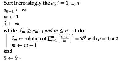
4. Graph Construction and Examples of Image Processing on Point Clouds

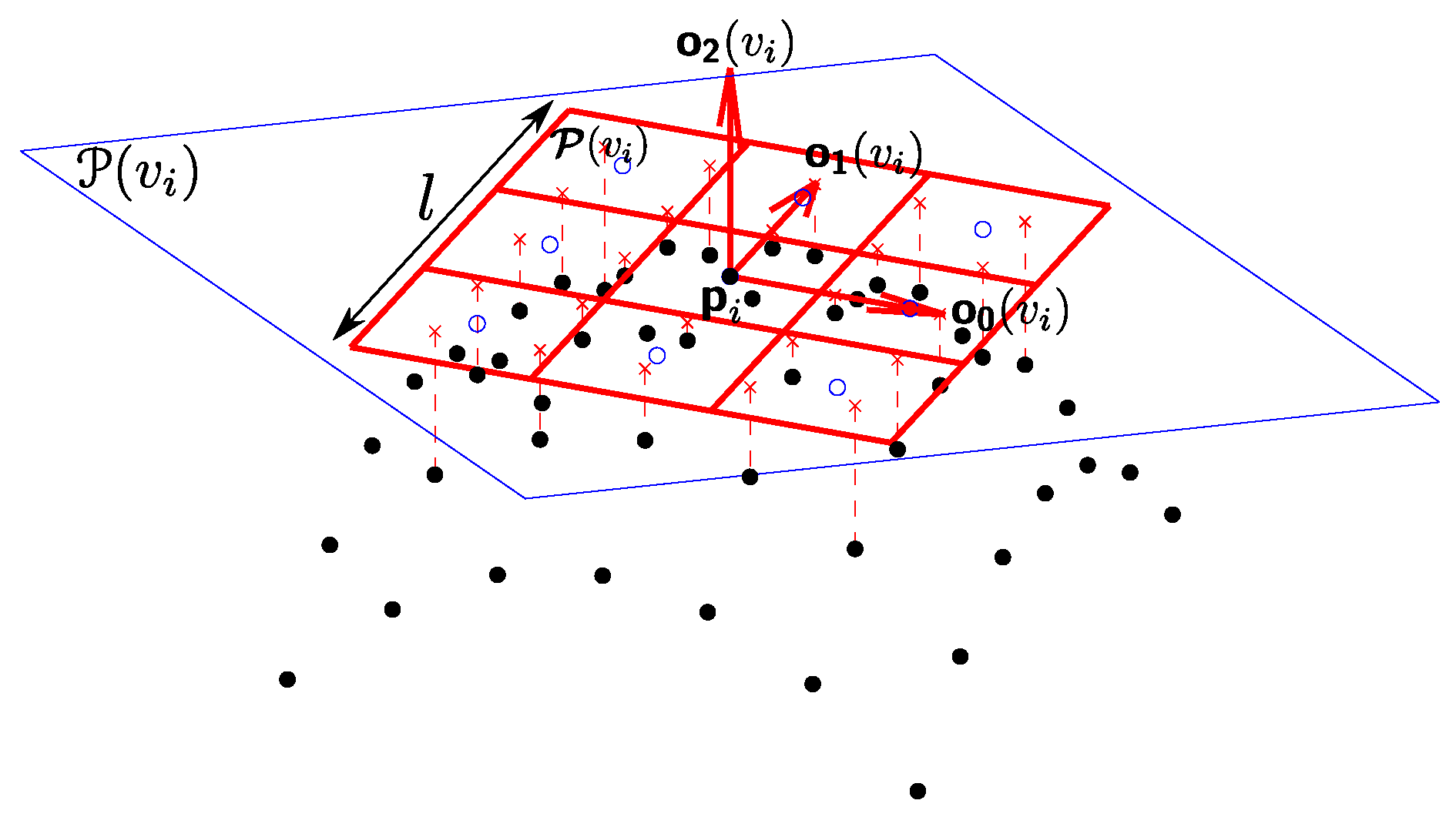
4.1. Graph Construction from Images on 3D Point Clouds

We consider a surface or a point cloud composed by a set S of vertices, such as S = { x 1 , x 2 , . . . } , with x i R 3 . To each raw point x i S , one associates a vertex of a graph G to define a set of vertices V. Data on the image or point cloud can be defined as a function f : V R . The construction of such a graph consists of modeling the neighborhood relationships between the data through the definition of a set of edges E and using a pairwise similarity measure μ : V × V I R + . In the particular case of images, edges based on geometric neighborhoods are particularly well-adapted to represent the geometry.
From a point cloud, a k-nn-graph is built. k controls the number of incident edges at each vertex and depends on the application. Generally, a low value (e.g., k = 5 ) is set for a local processing and a higher value for a non-local processing.
From a mesh, the set E is deduced from the implicit graph in the triangular mesh. The similarity between two vertices is computed by a similarity measure s : E I R + , which satisfies:
w ( u , v ) = s ( u , v ) , if   ( u , v ) E 0 , otherwise .
Common similarity functions are the following:
s 0 ( u , v ) 1 , s 1 ( u , v ) = exp ( μ ( f ( u ) , f ( v ) / σ 2 ,
for which the variance parameter σ > 0 usually depends on the variation of the function μ.
The function f used to describe the data at a vertex u is considered as the feature vector. Several choices can be considered for the expression of the feature vectors, depending on the nature of the features to be used for graph processing. In the context of image processing, one can use a simple gray scale or color feature vector F u or a patch feature vector F u τ = v W τ ( u ) F v (i.e., the set of values F v for which v is in a square window W τ ( u ) of size ( 2 τ + 1 ) × ( 2 τ + 1 ) centered at pixel u). Note that the latter vector allows one to incorporate nonlocal features for τ 1 . We now present our method for the construction of patches on surfaces and point clouds.
Patch construction for 3D point clouds: Extending the notion of a patch to three-dimensional point cloud data is not an easy task. In [21], we have proposed a novel definition of patches that can be used for any graph representation associated with meshes or point clouds. In particular, around each vertex, we build a two-dimensional grid (the patch) describing the close neighborhood. This grid is defined on the tangent plane of the point (i.e., the vertex). Then, the patch is oriented accordingly, and finally, the patch is filled in with a weighted average of the graph-signal values in the local neighborhood. The first step consists of estimating the orientation of each patch. The second step consists of the actual patch construction. The set of values inside the patch of the vertex u is denoted as P ( u ) . Let C k ( u ) denote the k-th cell of the constructed patch around u with k { 1 , , n 2 } . With the proposed patch construction process, one can define the set V k ( u ) = { v | p v C k ( u ) } as the set of vertices v that are assigned to the k-th patch cell of u. Then, the patch vector is defined as P ( u ) = v V k ( u ) w ( c k , p v ) f ( v ) v V k ( u ) w ( c k , p v ) k { 1 , , n 2 } T with w ( c k , p u ) = exp ( | | c k p u | | 2 2 σ 2 ) , for which c k is the vector of coordinates of the k-th patch cell center. This weighting enables us to take into account the point distribution within the patch cells in order to compute their mean feature vectors. Figure 1a summarizes our patch construction method.

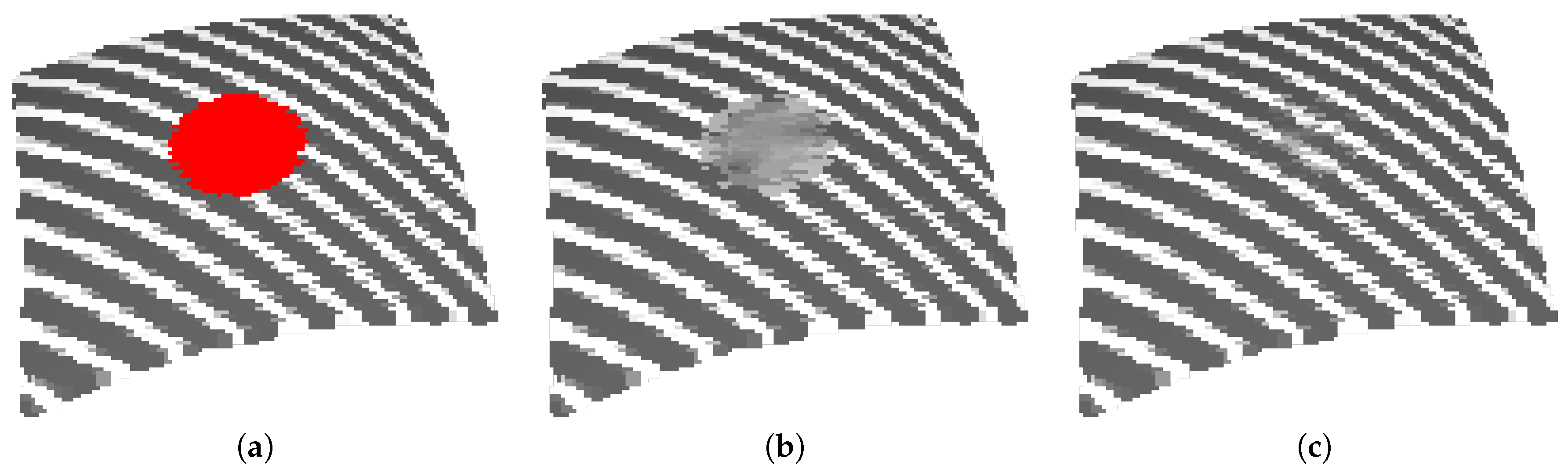
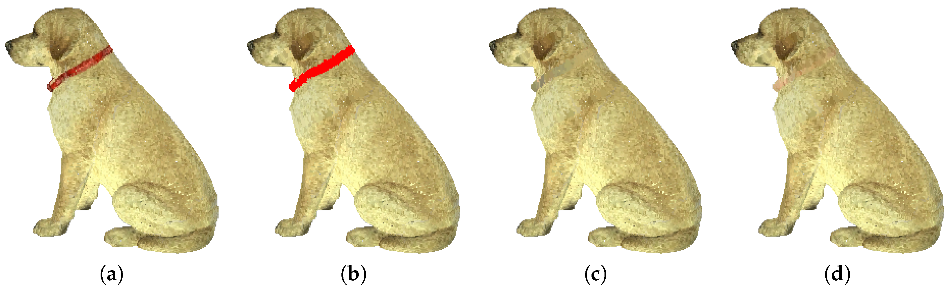
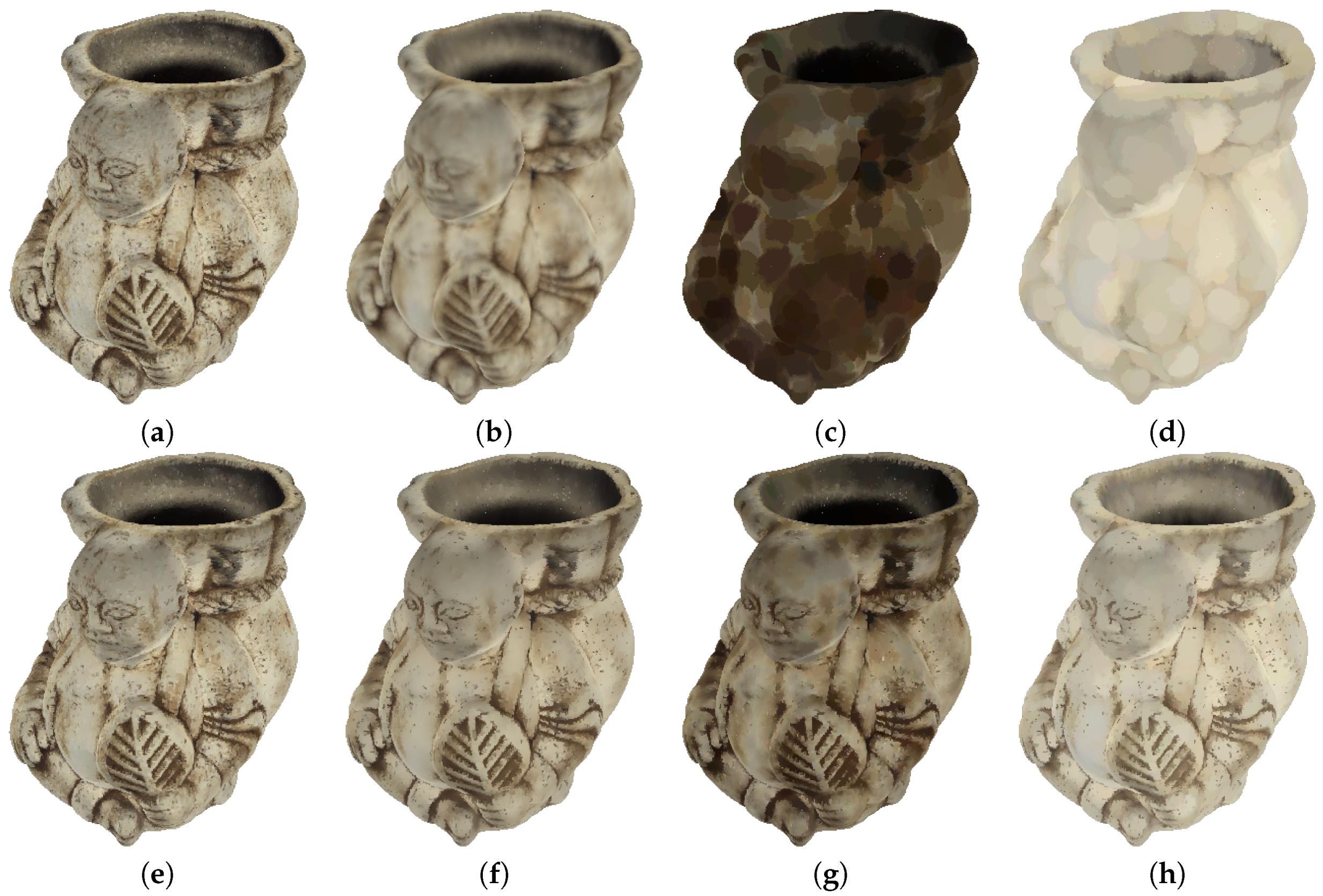
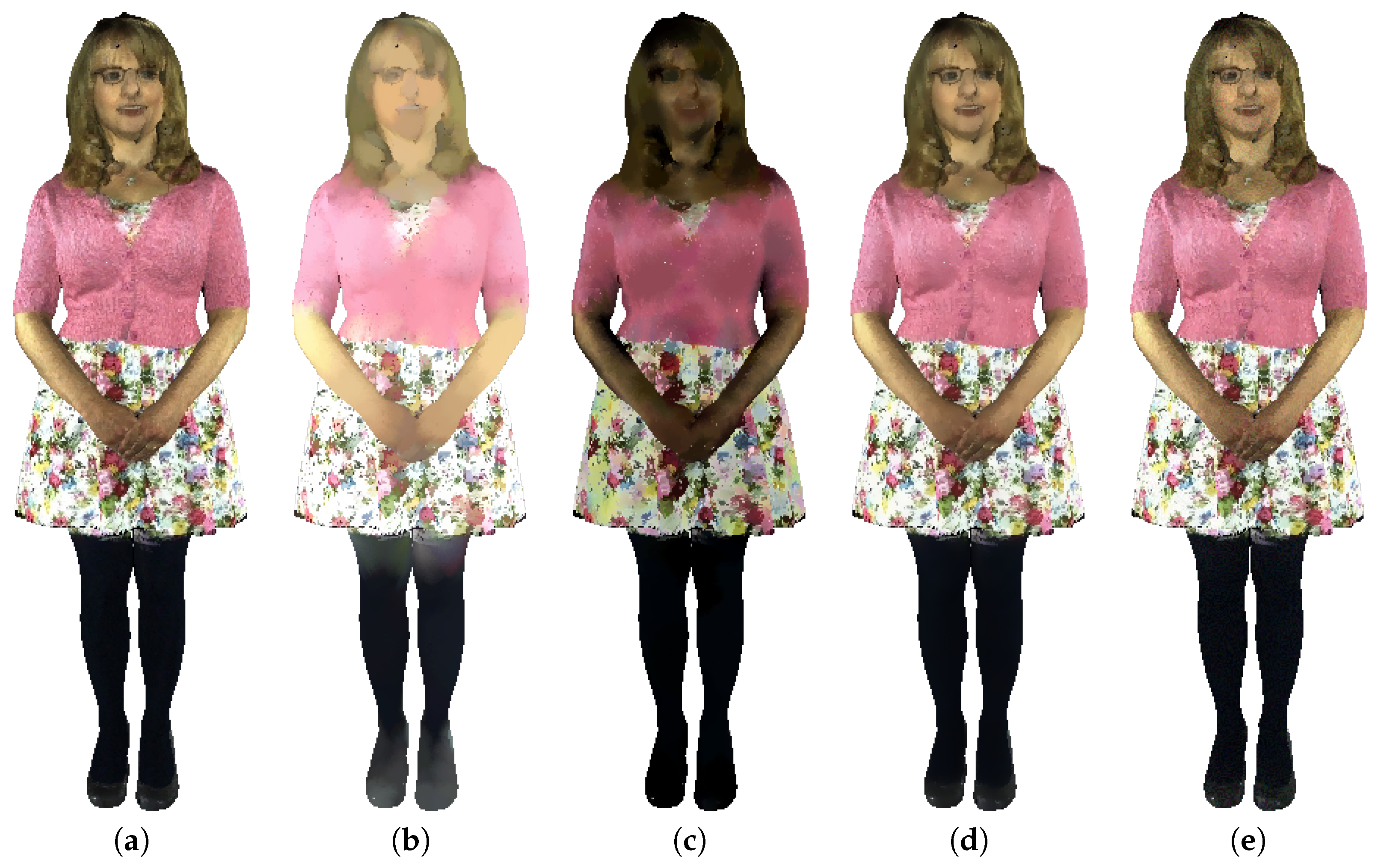
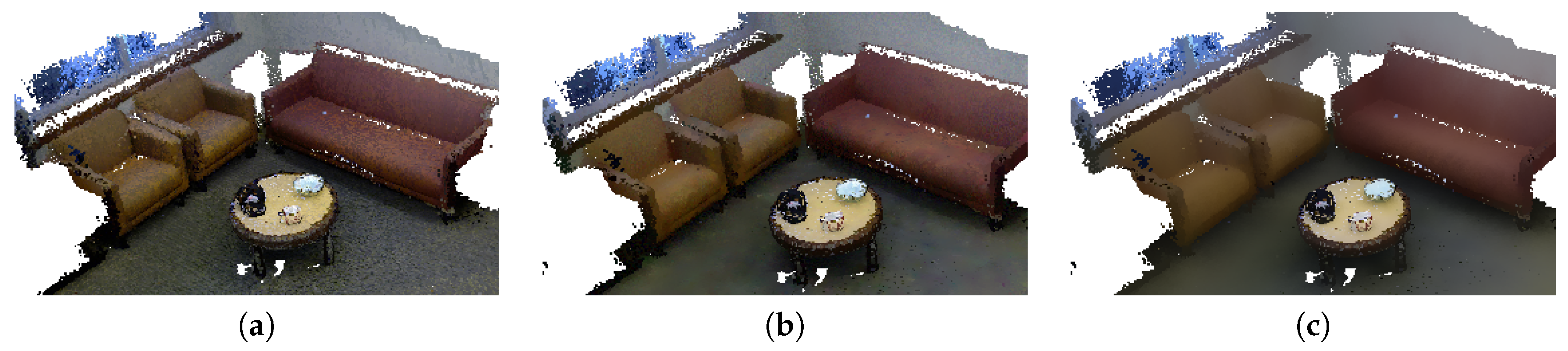
4.2. Local, Non-Local Inpainting and Filtering of Images on Point Clouds

In this section, we illustrate through some examples the application of morphological operators on graphs for inpainting, filtering of images on point clouds. All processing have been implemented in C++ and take almost several seconds on a current laptop running on a GNU/Linux operating system.
Inpainting: Image inpainting using a patch-based approach has been proposed by [38]. Recent works on inpainting tend to unify local and non-local approaches under a discrete or continuous variational formulation (for more details, see [39,40] and the references therein). Here, we consider that images on point clouds are defined on a general domain represented by an adaptive graph G = ( V , E , w ) . We consider both local and non-local inpainting as an interpolation problem. Let f 0 : V I R be an initial function. Let A V be the subset of vertices with unknown values and A the subset of vertices with known values. The purpose of inpainting is to find a function f extending f 0 in V by solving the ∞-Laplacian equation:
( Δ w , f ) ( u ) = 0 u A , f ( u ) = f 0 ( u ) u A .
The solution f is said to be infinity-harmonic [40].
The solution is obtained with this simple iterative algorithm based on the NLA operator introduced in Equation (40). At each iteration, only the internal boundary A = { u A | v u , v A } is interpolated:
{ N L A ( f ) ( u ) = 1 2 [ N L D ( f ) ( u ) + N L E ( f ) ( u ) ] u A , N L A ( f ) ( u ) = f 0 ( u ) u A .
At the end of each iteration, the set A is updated by A ( n + 1 ) = A ( n ) A ( n ) , and A ( n + 1 ) is updated from A ( n + 1 ) . The algorithm stops when the set of vertices to inpaint is empty.
{ f ( 0 ) ( u ) = f 0 ( u ) , f ( n + 1 ) ( u ) = N L A ( f ( n ) ) ( u ) .
Figure 2 shows the inpainting results of a synthetic textured point cloud with a constant ( w = 1 ) weight function defined locally (Figure 2b) and with a patch-based similarity metric defined on a non-local neighborhood (Figure 2c). The method presented in Section 4.1 has been used to construct the graph from the point cloud. Better results are obtained with non-local processing with the patch-based similarity measure. This weighting scheme captures texture information and is then able to interpolate repetitive patterns. Figure 3 shows an inpainting result of a colored point cloud acquired from a real object.
Filtering: We give some examples of filtering by local and non-local morphological operators: NLD (Non-Local Dilation), NLE (Non-Local Erosion), NLA (∞-Laplacian) and N L A 1 (mean curvature).
Figure 4 shows the filtering of a colored point cloud with the N L D , N L E and N L A operators. The weight functions w are computed from the colors of the point cloud. Results are shown with w 1 and w = 1 . When w 1 , denoising results are better since edges are preserved. Figure 5 shows the filtering of a colored point cloud with several operators. The N L A 1 operator defined in Equation (47) corresponds to a filtering operator by alternating the process of non-local dilation and non-local erosion according to the sign of the curvature K w on the graph Equation (21). When w = 1 , the filtering is unable to restore the colors on the point clouds. Figure 6 shows a comparison of the result obtained with the N L A and N L A 1 operators on a scanned room [41]. The N L A 1 operator produces better results by smoothing the colors while preserving details and contours, while the N L A operator smooths by removing many details.

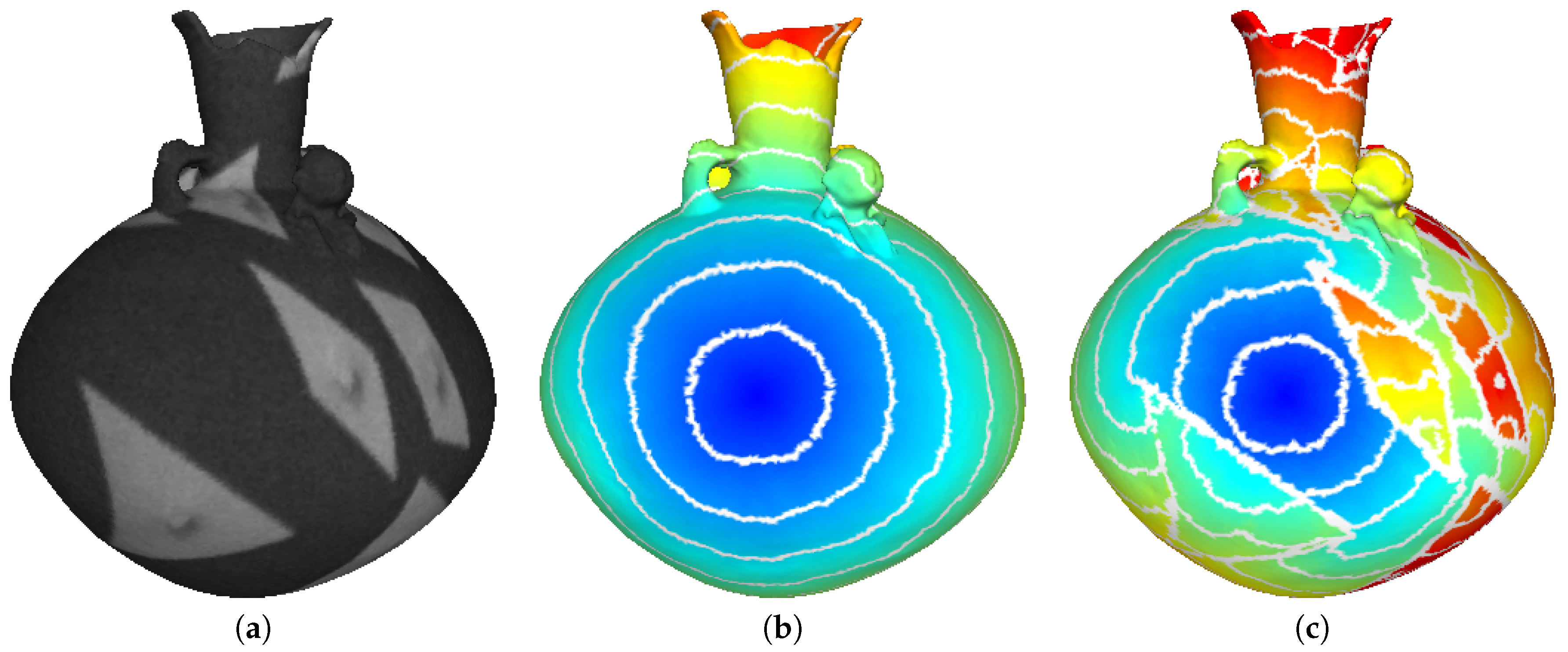
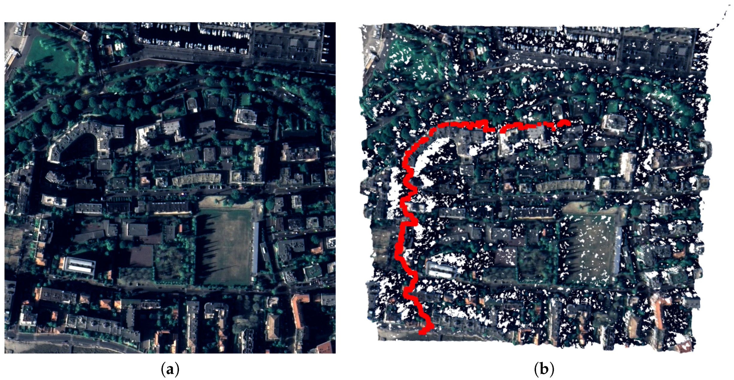
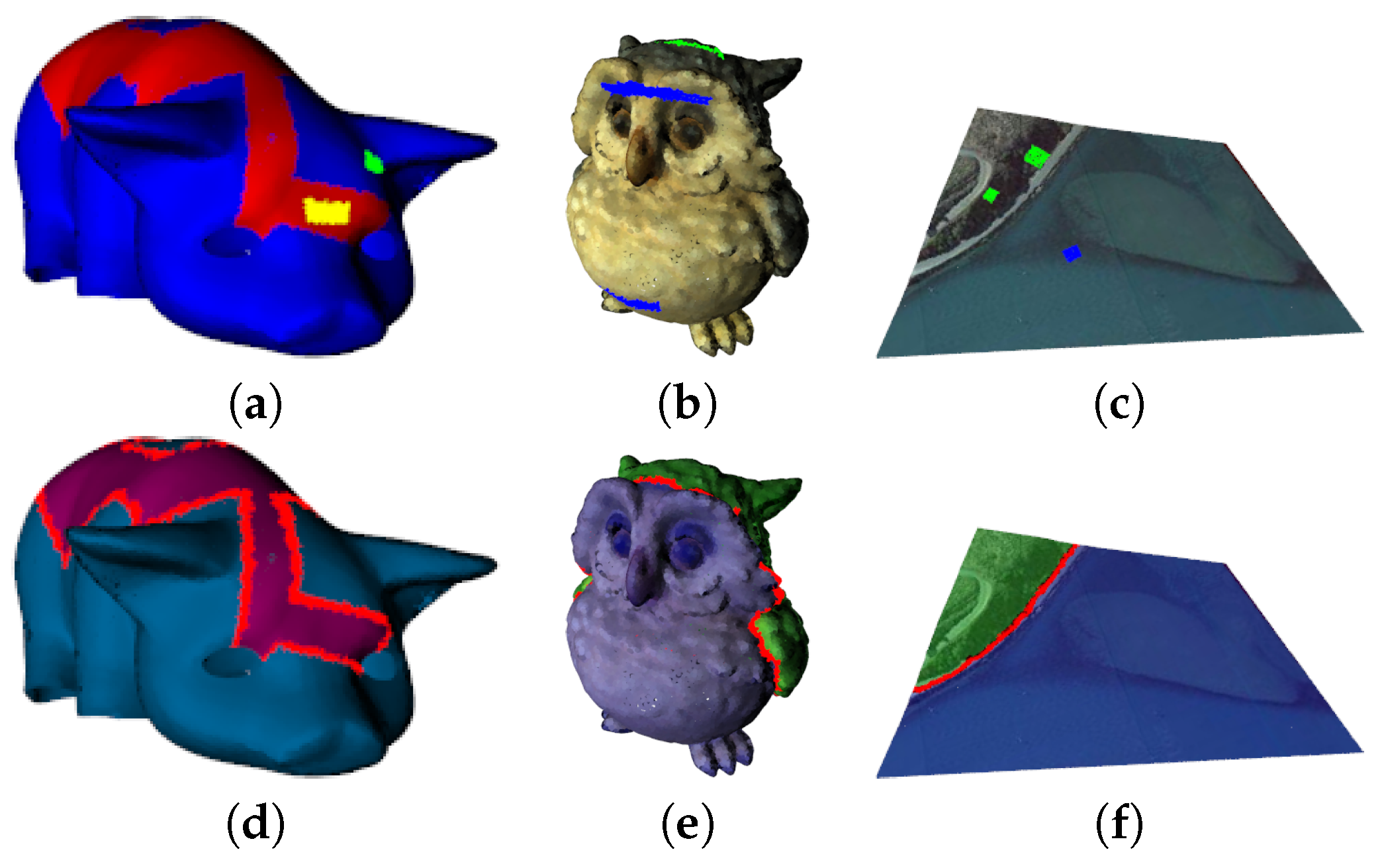
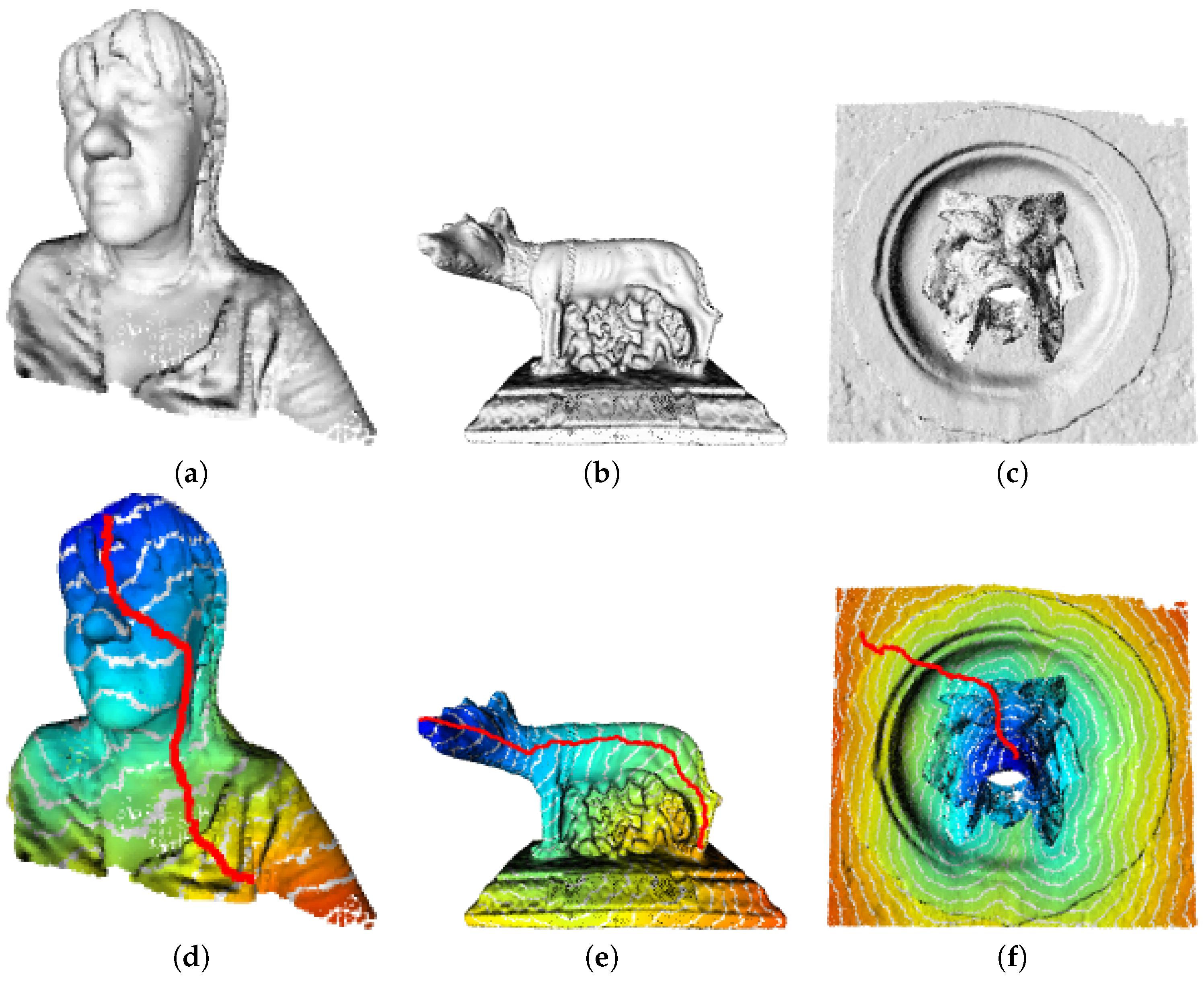
4.2.1. Generalized Weighted Distance, Shortest Path and Eikonal Equation for Segmentation of the Image on Point Clouds

The Eikonal equation defined in Equation (55) on a weighted graph of arbitrary topology allows one to compute generalized distances on graphs. We use the Eikonal equation with label propagation for computing the shortest path and segmentation on meshes or images painted on point clouds.
Generalized weighted distance: We compute the generalized distance on several point clouds by solving the Eikonal equation; see Figure 7. We built the graph as a k-nn with k = 5 , in the coordinate space of the point cloud. Since the spatial discretization step is regular enough, we use a constant weight function ( w ( u , v ) = 1 ). The superimposed red line on the figure is the shortest path between the source point (the point from which the distance is computed) and another point in the point cloud. This path was deformed using the computed distance function. Figure 8 shows the evolution of the distance estimation on a mesh from a vertex, with or without colorimetric constraints.
Figure 9 shows the shortest path between two points of a 3D city. This latter 3D point cloud has been generated from the online web interface to estimate colorized point clouds obtained from stereo satellite images [42]. The shortest path was obtained by processing the raw point cloud. Note that, even if the point cloud estimated is highly noisy and not uniform, the shortest path takes roads by nicely avoiding buildings. The result has been obtained with k = 10 .
Segmentation: Figure 10 shows the segmentation of a point cloud from colorimetric values. In Figure 8 and Figure 10, the similarity function w is computed from the color distance with w ( u , v ) = e | | f ( u ) f ( v ) | | 2 / σ 2 and f : V R the colorimetric function. Figure 11 shows the segmentation of meshes from the estimation of the geometric curvature; the similarity function is computed with w ( u , v ) = e ( K ( u ) K ( v ) ) 2 / σ 2 ; and K : V R the function that associates an estimation of the square of major principal curvature at each vertex u V . The estimation of the principal curvature is obtained by computing the eigenvalues as proposed in [43,44].

5. Conclusions

In this paper, we have adopted the PdE framework, and we have focused on some PDEs-based continuous morphological operators on Euclidean domains: dilation/erosion, mean curvature flows and the Eikonal equation. We have extended their applications for the processing of colored point clouds of geo-informatics 3D data. We briefly presented the construction of a graph from mesh or point cloud and show several examples, such as restoration, denoising, inpainting, object extraction or estimation of the minimal path. We have shown results on geographic data, such as the estimation of the shortest path on a raw point cloud of a 3D city or the segmentation of a LIDAR 3D point cloud based on the colorimetric values. The results demonstrated many potentials of the point cloud approach for the processing of geo-informatics 3D data.

Acknowledgments

This work was jointly supported by the PLANUCA project (funded under the Normandy Region and Europe FEDER) and the GRAPHSIP project (ANR).

Author Contributions

This is a collaboration work to extended applications for the processing of colored point clouds of geo-informatics 3D data using morphological PDEs on graphs. Abderrahim Elmoataz, François Lozes and Hugues Talbot have worked together to conceive, to perform the experiments and to write the paper.

Conflicts of Interest

The authors declare no conflict of interest.

References

  1. Osher, S.; Fedkiw, R. Level Set Methods and Dynamic Implicit Surfaces; Springer: New York, NY, USA, 2003; Volume 153. [Google Scholar]
  2. Sethian, J.A. Level Set Methods and Fast Marching Methods: Evolving Interfaces in Computational Geometry, Fluid Mechanics, Computer Vision, and Materials Science; Cambridge University Press: Cambridge, UK, 1999; Volume 3. [Google Scholar]
  3. Elmoataz, A.; Toutain, M.; Tenbrinck, D. On the p-Laplacian and ∞-Laplacian on Graphs with Applications in Image and Data Processing. SIAM J. Imaging Sci. 2015, 8, 2412–2451. [Google Scholar] [CrossRef]
  4. Elmoataz, A.; Lozes, F.; Toutain, M. Nonlocal PDEs on Graphs: From Tug-of-War Games to Unified Interpolation on Images and Point Clouds. J. Math. Imaging Vis. 2016. [Google Scholar] [CrossRef]
  5. Alvarez, L.; Guichard, F.; Lions, P.L.; Morel, J.M. Axioms and fundamental equations of image processing. Arch. Ration. Mech. Anal. 1993, 123, 199–257. [Google Scholar] [CrossRef]
  6. Elmoataz, A.; Desquesnes, X.; Lézoray, O. Non-Local Morphological PDEs and-Laplacian Equation on Graphs With Applications in Image Processing and Machine Learning. IEEE J. Sel. Top. Signal Process. 2012, 6, 764–779. [Google Scholar] [CrossRef]
  7. Maragos, P. Differential morphology and image processing. IEEE Trans. Image Process. 1996, 5, 922–937. [Google Scholar] [CrossRef] [PubMed]
  8. Meyer, F.; Maragos, P. Multiscale Morphological Segmentations Based on Watershed, Flooding, and Eikonal PDE. In Proceedings of the International Conference on Scale-Space Theories in Computer Vision, Corfu, Greece, 26–27 September 1999; pp. 351–362.
  9. Ta, V.T.; Elmoataz, A.; Lézoray, O. Nonlocal PDEs-based Morphology on Weighted Graphs for Image and Data Processing. IEEE Trans. Image Process. 2011, 26, 1504–1516. [Google Scholar]
  10. Dorninger, P.; Pfeifer, N. A Comprehensive Automated 3D Approach for Building Extraction, Reconstruction, and Regularization from Airborne Laser Scanning Point Clouds. Sensors 2008, 8, 7323–7343. [Google Scholar] [CrossRef]
  11. Wallace, L.; Lucieer, A.; Watson, C.; Turner, D. Development of a UAV-LiDAR System with Application to Forest Inventory. Remote Sens. 2012, 4, 1519–1543. [Google Scholar] [CrossRef]
  12. Jochem, A.; Höfle, B.; Rutzinger, M.; Pfeifer, N. Automatic Roof Plane Detection and Analysis in Airborne Lidar Point Clouds for Solar Potential Assessment. Sensors 2009, 9, 5241–5262. [Google Scholar] [CrossRef] [PubMed]
  13. Dandois, J.P.; Ellis, E.C. Remote Sensing of Vegetation Structure Using Computer Vision. Remote Sens. 2010, 2, 1157–1176. [Google Scholar] [CrossRef]
  14. Lai, R.; Chan, T.F. A framework for intrinsic image processing on surfaces. Comput. Vis. Image Underst. 2011, 115, 1647–1661. [Google Scholar] [CrossRef]
  15. Liang, J.; Lai, R.; Wong, T.W.; Zhao, H. Geometric Understanding of Point Clouds Using Laplace-Beltrami Operator. In Proceedings of the 2012 IEEE Conference on Computer Vision and Pattern Recognition (CVPR), Providence, RI, USA, 16–21 June 2012; pp. 214–221.
  16. Lai, R.; Liang, J.; Zhao, H. A local mesh method for solving PDEs on point clouds. Inverse Probl. Imaging 2013, 7, 737–755. [Google Scholar] [CrossRef]
  17. Stam, J. Flows on surfaces of arbitrary topology. ACM Trans. Graph. 2003, 22, 724–731. [Google Scholar] [CrossRef]
  18. Spira, A.; Kimmel, R. Geometric curve flows on parametric manifolds. J. Comput. Phys. 2007, 223, 235–249. [Google Scholar] [CrossRef]
  19. Bertalmio, M.; Cheng, L.; Osher, S.; Sapiro, G. Variational Problems and Partial Differential Equations on Implicit Surfaces. J. Comput. Phys. 2001, 174, 759–780. [Google Scholar] [CrossRef]
  20. Ruuth, S.J.; Merriman, B. A simple embedding method for solving partial differential equations on surfaces. J. Comput. Phys. 2008, 227, 1943–1961. [Google Scholar] [CrossRef]
  21. Lozes, F.; Elmoataz, A.; Lezoray, O. Partial Difference Operators on Weighted Graphs for Image Processing on Surfaces and Point Clouds. IEEE Trans. Image Process. 2014, 23, 3896–3909. [Google Scholar] [CrossRef] [PubMed]
  22. Lozes, F.; Elmoataz, A.; Lezoray, O. PDE-Based Graph Signal Processing for 3-D Color Point Clouds: Opportunities for cultural heritage. IEEE Signal Process. Mag. 2015, 32, 103–111. [Google Scholar] [CrossRef]
  23. Haralick, R.M.; Sternberg, S.R.; Zhuang, X. Image analysis using mathematical morphology. IEEE Trans. Pattern Anal. Mach. Intell. 1987, 9, 532–550. [Google Scholar] [CrossRef] [PubMed]
  24. Serra, J.; Soille, P. Mathematical Morphology and Its Applications to Image Processing; Springer Science & Business Media: Berlin, Germany, 2012; Volume 2. [Google Scholar]
  25. Angulo, J. Morphological PDE and Dilation/Erosion Semigroups on Length Spaces. In International Symposium on Mathematical Morphology and Its Applications to Signal and Image Processing; Springer: Cham, Switzerland, 2015; pp. 509–521. [Google Scholar]
  26. Crandall, M.G.; Lions, P.L. Viscosity solutions of Hamilton-Jacobi equations. Trans. Am. Math. Soc. 1983, 277, 1–42. [Google Scholar] [CrossRef]
  27. Maragos, P. Slope transforms: Theory and application to nonlinear signal processing. IEEE Trans. Signal Process. 1995, 43, 864–877. [Google Scholar] [CrossRef]
  28. Li, H.; Elmoataz, A.; Fadili, J.M.; Ruan, S. An improved image segmentation approach based on level set and mathematical morphology. In Proceedings of the Third International Symposium on Multispectral Image Processing and Pattern Recognition, Beijing, China, 20–22 October 2003; pp. 851–854.
  29. Osher, S.; Sethian, J.A. Fronts propagating with curvature-dependent speed: Algorithms based on Hamilton-Jacobi formulations. J. Comput. Phys. 1988, 79, 12–49. [Google Scholar] [CrossRef]
  30. Rouy, E.; Tourin, A. A viscosity solutions approach to shape-from-shading. SIAM J. Numer. Anal. 1992, 29, 867–884. [Google Scholar] [CrossRef]
  31. Pizarro, L.; Burgeth, B.; Breuß, M.; Weickert, J. A Directional Rouy-Tourin Scheme for Adaptive Matrix-Valued Morphology. In International Symposium on Mathematical Morphology and Its Applications to Signal and Image Processing; Springer: Berlin/Heidelberg, Germany, 2009; pp. 250–260. [Google Scholar]
  32. Breuß, M.; Weickert, J. A shock-capturing algorithm for the differential equations of dilation and erosion. J. Math. Imaging Vis. 2006, 25, 187–201. [Google Scholar] [CrossRef]
  33. Breuß, M.; Weickert, J. Highly Accurate PDE-Based Morphology for General Structuring Elements. In Proceedings of the International Conference on Scale Space and Variational Methods in Computer Vision, Voss, Norway, 1–5 June 2009; Springer: Berlin/Heidelberg, Germany, 2009; pp. 758–769. [Google Scholar]
  34. Burgeth, B.; Breuß, M.; Pizarro, L.; Weickert, J. PDE-Driven Adaptive Morphology for Matrix Fields. In Proceedings of the International Conference on Scale Space and Variational Methods in Computer Vision, Voss, Norway, 1–5 June 2009; pp. 247–258.
  35. Elmoataz, A.; Lezoray, O.; Bougleux, S. Nonlocal Discrete Regularization on Weighted Graphs: A Framework for Image and Manifold Processing. IEEE Trans. Image Process. 2008, 17, 1047–1060. [Google Scholar] [CrossRef] [PubMed]
  36. Bougleux, S.; Elmoataz, A.; Melkemi, M. Local and nonlocal discrete regularization on weighted graphs for image and mesh processing. Int. J. Comput. Vis. 2009, 84, 220–236. [Google Scholar] [CrossRef]
  37. Desquesnes, X.; Elmoataz, A.; Lézoray, O. Eikonal equation adaptation on weighted graphs: fast geometric diffusion process for local and non-local image and data processing. J. Math. Imaging Vis. 2013, 46, 238–257. [Google Scholar] [CrossRef]
  38. Efros, A.A.; Leung, T.K. Texture Synthesis by Non-Parametric Sampling. In Proceedings of the Seventh IEEE International Conference on Computer Vision, Kerkyra, Greece, 20–27 September 1999; Volume 2, pp. 1033–1038.
  39. Arias, P.; Facciolo, G.; Caselles, V.; Sapiro, G. A Variational Framework for Exemplar-Based Image Inpainting. Int. J. Comput. Vis. 2011, 93, 319–347. [Google Scholar] [CrossRef]
  40. Ghoniem, M.; Elmoataz, A.; Lézoray, O. Discrete Infinity Harmonic Functions: Towards a Unified Interpolation Framework on Graphs. In Proceedings of the 2011 18th IEEE International Conference on Image Processing (ICIP), Brussels, Belgium, 11–14 September 2011; pp. 1361–1364.
  41. Lai, K.; Bo, L.; Fox, D. Unsupervised Feature Learning for 3D Scene Labeling. In Proceedings of the IEEE International Conference on Robotics and Automation (ICRA), Hong Kong, China, 31 May–7 June 2014.
  42. De Franchis, C.; Meinhardt-Llopis, E.; Michel, J.; Morel, J.M.; Facciolo, G. An automatic and modular stereo pipeline for pushbroom images. ISPRS Ann. Photogramm. Remote Sens. Spat. Inf. Sci. 2014, 2, 49–56. [Google Scholar] [CrossRef]
  43. Berkmann, J.; Caelli, T. Computation of surface geometry and segmentation using covariance techniques. IEEE Trans. Patttern Anal. Mach. 1994, 16, 1114–1116. [Google Scholar] [CrossRef]
  44. Digne, J.; Morel, J.M. Numerical analysis of differential operators on raw point clouds. Numer. Math. 2014, 127, 255–289. [Google Scholar] [CrossRef]
Figure 1. Interpolation of the content of the patch with a patch length of l > 0 . o 0 ( u ) and o 1 ( u ) are the orientations of the patch P ( u ) at a point p u . Elements marked by a “×” symbol correspond to the projected neighbors p u of the point p u on the patch. These projections are used to deduce the values of each patch cell (a “o” symbol) by a weighted average of the associated graph signal values.
Ijgi 05 00213 g001
Figure 2. Inpainting of the color on a point cloud. (a) Point cloud to inpaint; (b) result of inpainting with w = 1 ; (c) result of inpainting with w based on the patch defined on point clouds (see Section 4.2).
Ijgi 05 00213 g002
Figure 3. Inpainting of the color on a point cloud. (a) Original point cloud; (b) point cloud to inpaint, where the red color represents points to inpaint; (c) result of inpainting with w = 1 ; (d) result of inpainting with the patch-based similarity metric (see Section 4.2).
Ijgi 05 00213 g003
Figure 4. Filtering of a colored point cloud with the N L D , N L D and N L A operators with k = 8 . (a) Original; (b) N L A w = 1 ; (c) N L E w = 1 ; (d) N L D w = 1 ; (e) N L A 0 w 1 ; (f) N L A w 1 ; (g) N L E w 1 ; (h) N L D w 1 . (bd,g,h) The results after 20 iterations. (e,f) The results after 200 iterations (see Section 4.2).
Ijgi 05 00213 g004
Figure 5. Filtering of a colored point cloud with several operators. Parameters are k = 8 , σ = 15 with 20 iterations for (ae) (see Section 4.2). (a) Original; (b) N L D ; (c) N L E ; (d) N L A ; (e) N L A 1 .
Ijgi 05 00213 g005
Figure 6. Filtering of a colored point cloud with N L A Equation (40) and N L A 1 Equation (47) operators after 500 iterations. The point cloud comes from RGB-D Scenes Dataset v2 [41]. (a) Original; (b) N L A 1 ; (c) N L A .
Ijgi 05 00213 g006
Figure 7. Geodesic distances on 3D point clouds with the Eikonal equation on the graph. (ac) show the original point clouds; (df) show the evolution of the distances with the minimal path linking two points of the point cloud. Blue and red color show low and high distances, respectively. White lines display isolines.
Ijgi 05 00213 g007
Figure 8. Generalized distance on the mesh with the Eikonal equation on the graph. From left to right: (a) original mesh; (b) result with w = 1 ; (c) result with w that depends on the vertices’ colors (see Section 4.2.1). Blue and red color show low and high distances, respectively. White lines display isolines.
Ijgi 05 00213 g008
Figure 9. Estimation of a shortest path on raw point clouds of a 3D city. The point cloud has been estimated from satellite images using [42]. From left to right: (a) one of the satellite images used to estimate the 3D point cloud; (b) 3D point cloud of a city, with the shortest path depicted in red.
Ijgi 05 00213 g009
Figure 10. Segmentation of 3D point clouds based on the colorimetric values by solving the Eikonal equation with P ( u ) = 1 (see Section 4.2.1). (ac) contain initial labels on point clouds. (df) show the results of the colorimetric segmentation, where red color represents the border between the blue and the green area.
Ijgi 05 00213 g010
Figure 11. Segmentation of 3D meshes based on the geometric principal curvatures by solving the Eikonal equation with P ( u ) = 1 (see Section 4.2.1). (a,b) show the square of major principal curvature (blue color for low values, red for high values); (c,d) show the initial labels on the 3D mesh; (e,f) show the results of the geometric segmentation.
Ijgi 05 00213 g011

