Efficient Geo-Computational Algorithms for Constructing Space-Time Prisms in Road Networks

Abstract

The Space-time prism (STP) is a key concept in time geography for analyzing human activity-travel behavior under various Space-time constraints. Most existing time-geographic studies use a straightforward algorithm to construct STPs in road networks by using two one-to-all shortest path searches. However, this straightforward algorithm can introduce considerable computational overhead, given the fact that accessible links in a STP are generally a small portion of the whole network. To address this issue, an efficient geo-computational algorithm, called NTP-A*, is proposed. The proposed NTP-A* algorithm employs the A* and branch-and-bound techniques to discard inaccessible links during two shortest path searches, and thereby improves the STP construction performance. Comprehensive computational experiments are carried out to demonstrate the computational advantage of the proposed algorithm. Several implementation techniques, including the label-correcting technique and the hybrid link-node labeling technique, are discussed and analyzed. Experimental results show that the proposed NTP-A* algorithm can significantly improve STP construction performance in large-scale road networks by a factor of 100, compared with existing algorithms.

1. Introduction

Time geography is powerful for analyzing human movements and activities through space and time [1]. Rather than predicting activity-travel behavior directly, time geography mainly focuses on the feasibility for an individual to participate in activities under various Space-time constraints [2]. At the core of time geography is the Space-time prism (STP) model, which depicts Space-time extents that can be physically reached by the individual from specified locations within a given time budget. This STP model has been widely used for various applications, such as measuring individual accessibility to urban services [3,4,5,6,7], and formulating activity-based models of travel demand [8,9,10,11].

Time geography was first introduced by Torsten Hägerstrand in the 1970s [1]. In the decades after its introduction, time geography faded somewhat into the background [12], mainly due to the lack of geo-computational algorithms and individual-level movement data. With the advances in geographical information science (GIS) technologies in the 1990s, the last two decades have witnessed a resurgence of time geography in the literature. Substantial research efforts have been made to improving STP models to represent individuals’ accessible Space-time extents in complex urban areas. Recognizing that human movements in urban areas are usually constrained by road networks, Miller [13] proposed a network-based STP (or called network-time prism, NTP) model. Other researchers further improved this NTP model by considering travel environment complexities, including turn restrictions [14], dynamic and heterogeneous traffic conditions [15,16] and travel time uncertainties [17,18]. Chen et al. [19] extend the NTP model into public transit networks. A geo-computational algorithm was developed to efficiently construct STPs in public transit networks using the A* and branch-and-bound techniques. Several useful tools also have been developed for visually analyzing NTPs in real road networks [20,21,22].

In recent years, there has been a wider resurgence of time-geographic studies due to the emerging spatiotemporal big data, collected by a variety of geospatial technologies, including human and vehicle trajectories collected by GPS (Global Positioning System) devices, mobile phone records, smart card data, social media check-ins, etc. These spatiotemporal big data provide an unprecedented opportunity for time-geographic studies to uncover people’s mobility patterns and their interactions with the urban environment [23,24,25,26,27,28,29,30]. To support such time-geographic studies in the era of spatiotemporal big data, efficient geo-computational algorithms for constructing NTPs in large-scale road networks are sorely needed.

In most previous time-geographic studies, NTPs are constructed by a straightforward algorithm [31], which utilizes two one-to-all shortest path searches, based on the Dijkstra’s algorithm. This straightforward algorithm is hereafter referred to as the NTP-Dij algorithm for convenience. In the NTP-Dij algorithm, a forward shortest path search is firstly carried out from the origin to determine the earliest arrival time at every node. Then, a backward shortest path search is performed from the destination to obtain the latest departure time at every node. Finally, the accessible nodes (and links) can be determined by checking whether their earliest arrival time is larger than the latest departure time. Such a NTP-Dij algorithm is easy to implement by directly using the classical shortest path algorithm (i.e., Dijkstra’s algorithm). However, it requires exploration of the whole network twice, and leads to considerable computational overheads, given the fact that accessible nodes in the NTP are generally only a small portion of the entire network. To reduce the number of explored nodes, Kuijpers and Othman [28,29] proposed an algorithm (called NTP-SN in this study) to construct the NTP in a sub-network instead of the whole network. The sub-network is generated by selecting nodes and links within the STP in the planar space. Nevertheless, the computational advantage of this NTP-SN algorithm is marginal, because the STP in the planar space is generally quite large compared with the actual NTP [28,29]. Further, although several NTP construction algorithms have been developed, there is a lack of numerical experiments in the literature to systematically investigate the computational performance of existing NTP construction algorithms in real road networks.

To fill this gap, this study investigates models and geo-computational algorithms for efficiently constructing NTPs in real road networks. This study contributes to time-geography literature in the following aspects:

Firstly, an improved NTP model is proposed by considering the complexities of road networks, including turn restrictions and divided/undivided roads. The proposed NTP model differentiates divided and undivided roads, and allows for individuals to make U-turns and access partial links on undivided roads. The proposed model, thus, enhances the realistic representation of NTPs in road networks.

Secondly, an efficient geo-computational algorithm, called NTP-A*, is developed to construct NTPs in large-scale road networks. In the proposed NTP-A* algorithm, turn restrictions and partially accessible links on undivided roads are explicitly considered. The A* and branch-and-bound techniques are employed to improve the NTP construction performance by discarding inaccessible links during shortest path searches. The label-correcting and hybrid link-node labeling techniques are also introduced in order to improve the NTP construction performance. The proposed NTP-A* algorithm, therefore, significantly improves the NTP construction performance in large-scale road networks.

Thirdly, a comprehensive case study using several real road networks is carried out to examine the computational performance of the proposed NTP-A* algorithm. Two existing NTP construction algorithms, NTP-Dij and NTP-SN, are also implemented for comparison purposes. Several implantation techniques (including the A* technique, branch-and-bound technique, label-correcting technique and hybrid link-node labeling technique) in the NTP construction are examined and discussed. The results of the case study indicate that the proposed NTP-A* algorithm can significantly improve the existing NTP-Dij and NTP-SN algorithms by a factor of 100 in large-scale road networks.

The remainder of this paper is structured as follows. In the next section, the classical STP model in the planar space is briefly introduced to provide a necessary background. The improved NTP model is introduced in Section 3. The proposed NTP-A* algorithm is presented in Section 4. Computational experiments using real-world road networks are reported in Section 5. Finally, the conclusions and future research recommendations are given in Section 6.

2. The Classical Space-Time Prism Model in the Planar Space

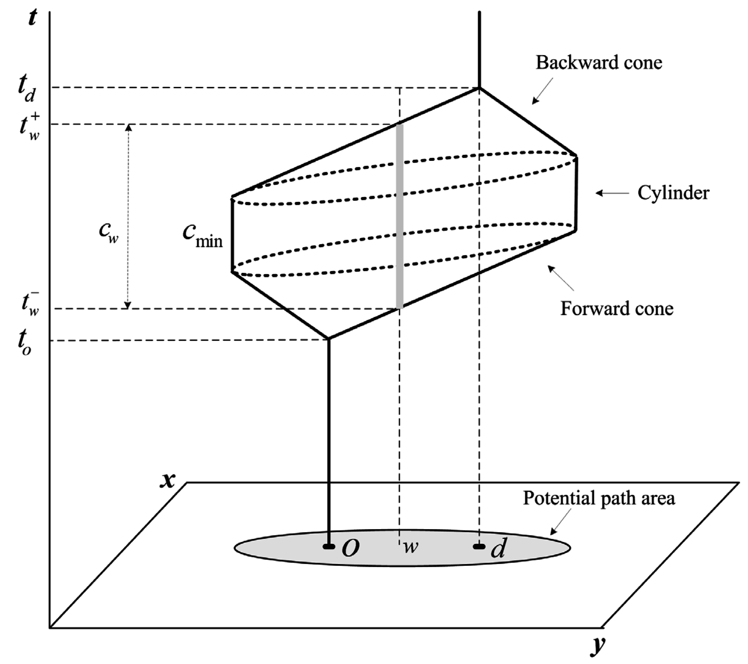
This section briefly introduces the classical Space-time prism (STP) model in the planar space. Figure 1 illustrates this prism model in a three-dimensional (3D) space, where the x and y axes represent two-dimensional (2D) geographic space and the t axis represents time. Suppose an individual planning to conduct two fixed activities at origin $o=(x_o,y_o)$ and time instance $t_o$, and destination $d=(x_d,y_d)$ and time instance $t_d$, respectively. The STP delimits Space-time extents for the individual to schedule another flexible activity between these two fixed activities. Analytically, the STP can be constructed by the intersection of a forward cone, a backward cone, and a cylinder. The forward cone, $\text{FC}(\mathrm{t})$, consists of all locations that can be reached from the origin at time $t$; the backward cone, $\text{BC}(\mathrm{t})$, comprises all locations that can arrive at the destination given the remaining time $t_s-t$; and the cylinder, $\text{CY}(\mathrm{t})$, delimits all geographic locations within the potential path area (PPA). According to Reference [2], the STP in the planar space can be formally expressed as

$$\text{STP}(\mathrm{t})=\text{FC}(\mathrm{t})\cap \text{BC}(\mathrm{t})\cap \text{CY}(\mathrm{t})$$

(1)

$$\text{FC}(\mathrm{t})=\{w|t\ge t_o+t_E^{ow},t\le t_d\}$$

(2)

$$\text{BC}(\mathrm{t})=\{w|t\le t_d-t_E^{wd},t\ge t_o\}$$

(3)

$$\text{CY}(\mathrm{t})=\{w|t_E^{ow}+t_E^{wd}\le t_d-t_o-c_{\text{min}},t_o\le t<t_d\}$$

(4)

where $c_{\text{min}}$ is the minimum duration for flexible activity participations, $t_E^{ow}$ is the Euclidean travel time from the origin to a location $w=(x_w,y_w)$, and $t_E^{wd}$ is the Euclidean travel time from the location $w$ to the destination. In the planar space, the Euclidean travel times (i.e., $t_E^{ow}$ and $t_E^{wd}$) can be calculated simply as Euclidean distances (denoted by $d_E^{ow}$ and $d_E^{wd}$) between these two locations divided by the maximum travel speed $v^{\text{max}}$.

Projecting the STP onto the 2D geographical space forms a PPA that includes all accessible locations for flexible activity participations in the 2D geographic space as:

$$PPA=\{w|t_E^{ow}+t_E^{wd}\le b\}$$

(5)

where $b=t_d-t_o-c_{\text{min}}$ is the maximum time budget for traveling. The height of the Space-time prism at location $w$ represents the maximum activity duration, $c_w$, at the location as:

$$c_w=t_w^{+}-t_w^{-}=(t_d-t_E^{wd})-(t_o+t_E^{ow})$$

(6)

where $t_w^{-}=t_o+t_E^{ow}$ is the earliest arrival time at the location, and $t_w^{+}=t_d-t_E^{wd}$ is the latest departure time from the location.

The above classical STP model in the planar space can be easily constructed and have rigorous formalization. However, this model builds on an unrealistic assumption that movements occur at a constant speed everywhere in the planar space [2,12,13,15]. In reality, people in urban areas do not move freely in the planar space, but, rather, within spatially embedded road networks. The classical STP model, thus, oversimplifies real travel environment complexities, and is inadequate for an individual’s activity-travel scheduling.

3. Constructing Space-Time Prisms in Road Networks

This section formulates a network-time prism (NTP) model, considering the complexities of road networks, including turn restrictions and divided/undivided roads. A road network can be represented as a directed graph $G(N,A,\Psi )$, comprising a set of nodes $N$, a set of links $A$, and a set of allowed turns $\Psi$. Each directed link $a_{ij}\in A$ has a tail node $i$, a head node $j$, and a link travel time $t_{ij}$. A turn ${\psi }_{ijk}\in \Psi$, passing through links $a_{ij}$ and $a_{jk}$, represents an allowed movement at node $j$ (e.g., right turn or U-turn). 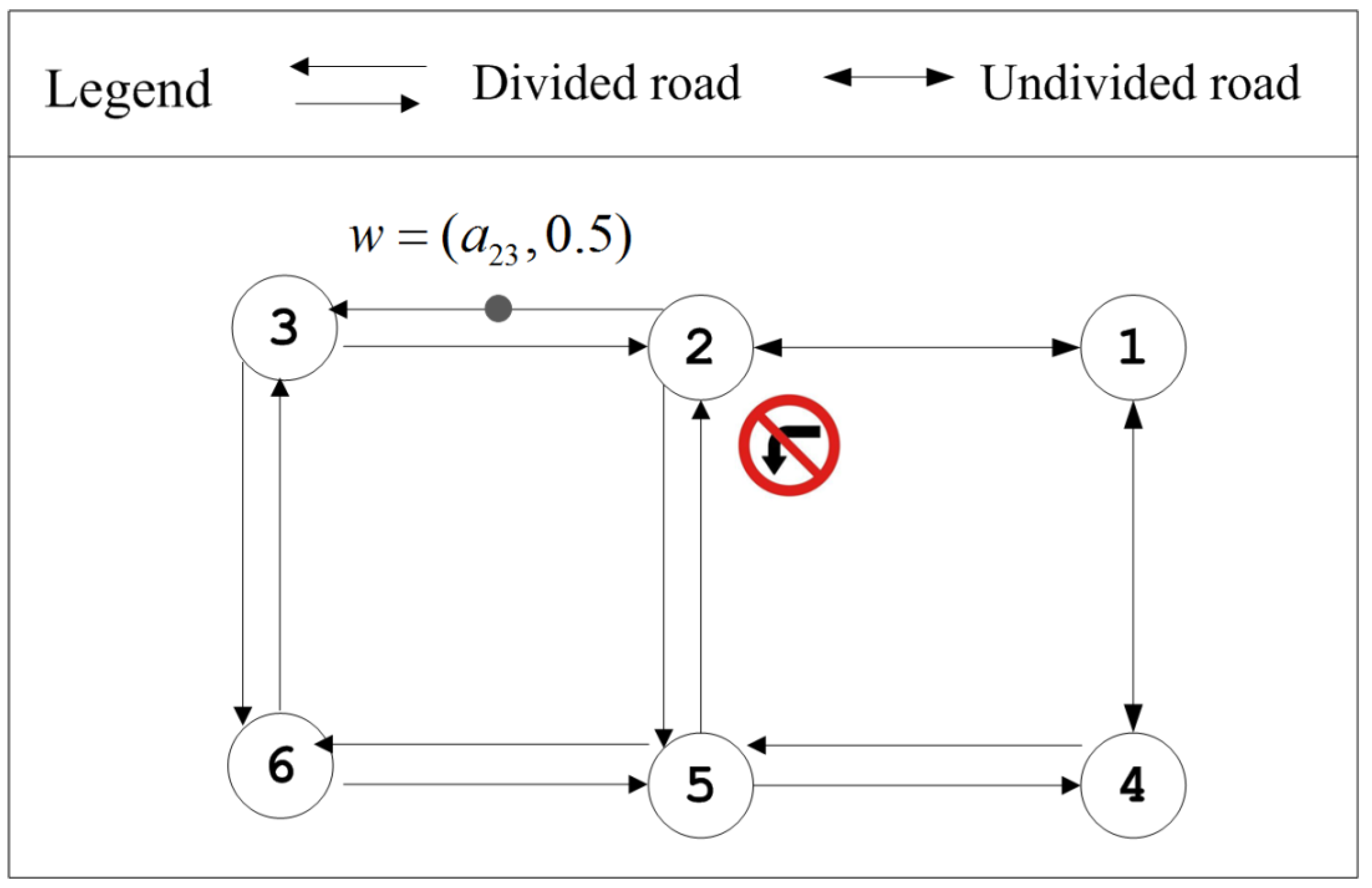Further, ${\psi }_{ijk}\notin \Psi$ means that the movement from link $a_{ij}$ to link $a_{jk}$ is restricted at node $j$ (e.g., left turn ${\psi }_{125}$ in Figure 2). In addition to making turns at nodes, U-turns are allowed at any location on an undivided link (e.g., a minor road), but restricted on a divided link (e.g., an arterial road). For example, $a_{12}$ and $a_{21}$ in Figure 2 are two opposite links of an undivided road, and travelers can freely make U-turns between these two links. It should be noted that a two-way road, regardless of whether it is divided or undivided, is represented by two opposite directed links, while a one-way road is represented by only one directed link.

Any location $w=(x_w,y_w)$ in the network can be represented as $(a_{ij},{\theta }_w)$ using the linear reference technique [23,32], where ${\theta }_w\in [0,1]$ is the relative position on the link $a_{ij}\in A$. For example, location $w=(a_{23},0.5)$ in Figure 2 indicates the middle of link $a_{23}$. The travel times of partial links $a_{iw}$ and $a_{wj}$ are assumed to be proportional to their distance as:

$$t_{iw}={\theta }_w{t}_{ij}$$

(7)

$$t_{wj}=(1-{\theta }_w)t_{ij}$$

(8)

Let $p_R^{wl}$ be the least time path between two locations, $w=(x_w,y_w)$ and $l=(x_l,y_l)$. The path travel time, $t_R^{wl}$, can be calculated by summing the corresponding link travel times along the path:

$$t_R^{wl}={\displaystyle \sum _{\forall a_{ij}}{t}_{ij}}{\delta }_{ij}^{wl}$$

(9)

where ${\delta }_{ij}^{wl}$ is the link-path incidence relationship, ${\delta }_{ij}^{wl}=1$ means that (partial) link $a_{ij}$ is on path $p_R^{wl}$, and otherwise ${\delta }_{ij}^{wl}=0$. In the road network with turn restrictions, the least time path can be determined by shortest path algorithm using a link-based labeling technique [33]. It should be noted that the classical node-based Dijkstra’s algorithm [34] ignores turn restrictions and may lead to infeasible paths.

Let $t_R^{ow}$ be the least travel time from the origin to location $w$, and let $t_R^{wd}$ be the least travel time from location $w$ to the destination. By replacing $t_R^{ow}$ and $t_R^{wd}$ with $t_E^{ow}$ and $t_E^{wd}$ in Equations (1)–(4), the NTP in the road network can be expressed as

$$\text{NTP}(\mathrm{t})=\text{FC}(\mathrm{t})\cap \text{BC}(\mathrm{t})\cap \text{CY}(\mathrm{t})$$

(10)

$$\text{FC}(\mathrm{t})=\{w|t\ge t_o+t_R^{ow},t\le t_d\}$$

(11)

$$\text{BC}(\mathrm{t})=\{w|t\le t_d-t_R^{wd},t\ge t_o\}$$

(12)

$$\text{CY}(\mathrm{t})=\{w|t_R^{ow}+t_R^{wd}\le t_d-t_o-c_{\text{min}},t_o\le t<t_d\}$$

(13)

This NTP delimits an individual’s accessible Space-time locations in the road network between origin $o=(a_o,{\theta }_o)$ and destination $d=(a_d,{\theta }_d)$ during the time period of $t_o$ to $t_d$. The height of the NTP at location $w$ represents the maximum activity duration $c_w$ at the location as:

$$c_w=t_w^{+}-t_w^{-}=(t_d-t_R^{wd})-(t_o+t_R^{ow})$$

(14)

where $t_w^{-}=t_o+t_R^{ow}$ and $t_w^{+}=t_d-t_R^{wd}$, respectively, are the earliest arrival time and the latest departure time from the location.

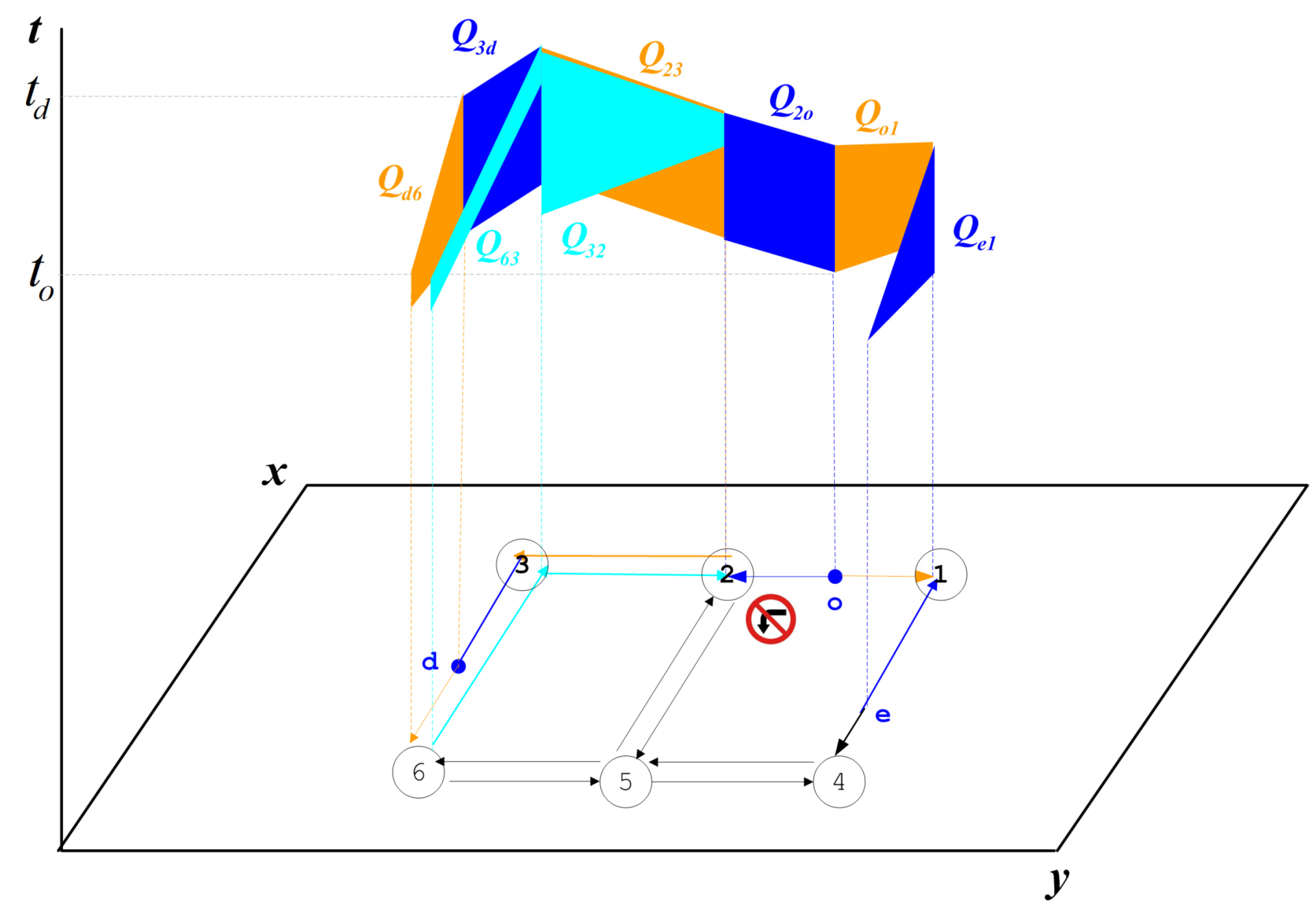
Figure 3 illustrates a simple NTP in a road network. As can be seen in the figure, the NTP comprises a set of 2D Space-time polygons $\{\dots ,Q_{ij}\dots \}$ on network links. Each Space-time polygon $Q_{ij}=\{(x_i,y_i,t_i^{+}),\dots ,(x_j,y_j,t_j^{+}),(x_j,y_j,t_j^{-}),\dots ,(x_i,y_i,t_i^{-})\}$ represents all accessible Space-time locations along network link $a_{ij}$ [23]. The projection of the NTP onto the 2D geographic space is the potential network area (PNA), comprising a set of accessible (partial) links $\{\dots ,a_{ij}\dots \}$. Let $p_R^{oj}$ be the least time path from origin $o$ to node $j$ passing through link $a_{ij}$, and let $p_R^{id}$ be the least time path from node $i$ to destination $d$ passing through link $a_{ij}$. Their path travel times are $t_R^{oj}$ and $t_R^{id}$, respectively. Accessible link $a_{ij}\in PNA$ should satisfy following travel time budget constraint:

$$t_R^{oj}+t_R^{id}-t_{ij}\le b=t_d-t_o-c_{\text{min}}$$

(15)

It can be observed from Figure 3 that divided and undivided links could have significant differences in their 2D polygons. Firstly, identical Space-time polygons can be generated on two opposite links of an undivided road, but not a divided road. For example, origin $o=(a_{12},0.5)$ in the figure is located on undivided link $a_{12}$. Since travelers can make U-turns freely on the undivided road, identical Space-time polygons (i.e., $Q_{o2}=Q_{2o}$ and $Q_{o1}=Q_{1o}$) are generated on opposite links $a_{12}$ to $a_{21}$. The situation is, however, different for destination $d=(a_{36},0.5)$, located on divided link $a_{36}$. As travelers cannot make U-turns at divided links, different shapes of Space-time polygons (i.e., $Q_{63}\ne Q_{3d}$ and $Q_{63}\ne Q_{d6}$) are generated on opposite links $a_{36}$ to $a_{63}$. Secondly, partial links within the NTP can be observed only on undivided roads and not on divided roads. For example, it can be seen from the figure that Node 1 is within the PNA, but Node 4 is not. As link $a_{14}$ is undivided, travelers can access part of the locations on the link and turn back to Node 1; and, thus, partial links $a_{1e}$ and $a_{e1}$ are accessible with Space-time polygons $Q_{1e}$ and $Q_{e1}$. It can also be seen from the figure that partial links are not accessible for divided links $a_{56}$ and $a_{65}$. Although Node 6 is accessible within the PNA, travelers cannot reach other locations at the link and return to Node 6 by making U-turns on the divided link. Therefore, divided and undivided links can have significantly different Space-time polygons and should be explicitly considered in the NTP model.

4. Geo-Computational Algorithms for Constructing Network-Time Prisms

Similar to the existing NTP-Dij algorithm [6,31], a straightforward algorithm for constructing a NTP is to apply two shortest path searches using the link-based one-all Dijkstra’s algorithm [33]. The forward search is used to calculate the least travel time $t_R^{oj}$ from origin $o$ to every link $a_{ij}$ (i.e., head node $j$). The backward search is to calculate the least travel time $t_R^{id}$ from every link $a_{ij}$ (i.e., tail node $i$) to destination $d$. Then, accessible links $\forall a_{ij}\in PNA$ satisfying $t_R^{oj}+t_R^{id}-t_{ij}\le b$ can be identified. This straightforward algorithm is easy to implement by directly using the existing link-based Dijkstra’s algorithm. However, it can lead to considerable computational overheads by exploring all network links twice, given the fact that accessible links in the NTP are generally a small portion of the entire network.

In this study, an efficient algorithm (called the NTP-A* algorithm) is proposed by using A* and branch-and-bound techniques. The A* technique, utilizing a heuristic evaluation function, is proved to be effective in improving shortest path search performance. The branch-and-bound technique tries to discard inaccessible links $\forall a_{ij}\notin PNA$ (i.e., $t_R^{oj}+t_R^{id}-t_{ij}>b=t_d-t_o-c_{\text{min}}$) during forward and backward shortest path searches, rather than after the shortest path searches. Using these two techniques, the proposed NTP-A* algorithm can significantly reduce the number of explored links by the two shortest path searches and can thereby improve the NTP construction performance. The detailed steps of the NTP-A* algorithm are described below.

Step 1. Road network modification. In classical shortest path algorithms, the origin and destination should be located at network nodes. This step is to address the situation of the origin at link $a_{ij}$ (destination at link $a_{uv}$) by adding temporary node $o$ ($d$) and links $a_{io}$ and $a_{oj}$ ($a_{ud}$ and $a_{dv}$) into network $G$. If link $a_{ij}$ ($a_{uv}$) is an undivided link, additional temporary links $a_{oi}$ and $a_{jo}$ ($a_{du}$ and $a_{vd}$) are also added in the opposite direction.

Step 2. Forward shortest path search. This step is to determine the least travel time $t_R^{oj}$ from the origin to each network link $a_{ij}$ by using the following R-FSP procedure (Road–Forward Search Procedure). Using the A* technique, a heuristic evaluation function $F(j)=t_R^{oj}+h(j)$ is used as heuristic cost for the forward shortest path $p_R^{oj}$ from the origin to link $a_{ij}$, where $h(j)$ is the estimated lower bound of $t_R^{id}-t_{ij}$. Since the Euclidean travel time $t_E^{jd}$ from node $j$ to the destination always satisfies $t_E^{jd}\le t_R^{id}-t_{ij}$, this study adopts $t_E^{jd}$ as the admissible $h(j)$ value. The $t_E^{jd}$ in the planar space can be calculated by $d_E^{jd}/v_R^{\text{max}}$, where $v_R^{\text{max}}$ is the maximum travel speed in the road network. Using the A* technique, the information of each link to the destination can be fully utilized to guide the forward shortest path search. The branch-and-bound technique is further incorporated in the forward search to discard all paths $p_R^{oj},\forall a_{ij}\in A$ satisfying $F(j)=t_R^{oj}+t_E^{jd}>b$. Because $t_R^{oj}+t_R^{id}-t_{ij}\ge F(j)=t_R^{oj}+t_E^{jd}$ always holds, all paths satisfying $F(j)>b$ can be identified as inaccessible links outside the NTP, and thus can be eliminated during the forward search. In this way, the forward search explores only a part of links $p_R^{oj}\ne \varphi ,\forall a_{ij}\in A$; other links $p_R^{oj}=\varphi ,\forall a_{ij}\in A$ outside the NTP are not explored.

R-FSP Procedure

Inputs: origin $o$ and destination $d$, travel time budget $b$

Outputs: the least travel times at accessible links

Step 1. Initialization:

01: For each link $a_{ij}\in A$

02:    Set forward path $p_R^{oj}:=\varphi$, its travel time $t_R^{oj}:=\infty$ and heuristic cost $F(j):=\infty$.

03: End For

04: For each link $a_{oj}$ emanating from origin $o$

05:    Create a forward path $p_R^{oj}:=a_{oj}$, and set $t_R^{oj}:=t_{oj}$ and $F(j):=t_{oj}+t_E^{jd}$.

06:    Insert $p_R^{oj}$ into the scan eligible $SE:=SE\cup \{p_R^{oj}\}$.

07: End For

Step 2. Path selection:

08: If $SE=\varphi$, then stop; otherwise, continue.

09: Select $p_R^{oi}$ at the top of $SE$, and remove it from $SE:=SE-\{p_R^{oi}\}$.

Step 3. Path extension:

10: For each allowed movement ${\psi }_{kij}$ from selected link $a_{ki}$ to link $a_{ij}$

11:    Create a forward path ${\widehat{p}}_R^{oj}:=p_R^{oi}\oplus a_{ij}$, and set ${\widehat{t}}_R^{oj}:=t_R^{oi}+t_{ij}$ and $F(j):={\widehat{t}}_R^{oj}+t_E^{jd}$.

12:    If $F(j)\le b$ then

13:     If ${\widehat{t}}_R^{oj}$ is less than the existing path travel cost $t_R^{oj}$ then

14:      If existing path $p_R^{oj}\in SE$, then set $SE:=SE-\{p_R^{oj}\}$.

15:      Set $p_R^{oj}:={\widehat{p}}_R^{oj}$ and $SE:=SE\cup \{{\widehat{p}}_R^{oj}\}$.

16:     End If

17:    End If

18: End For

19: Go back to Step 2.

Step 3. Backward shortest path search. This step is to determine the least travel time $t_R^{id}$ from each network link $a_{ij}$ to the destination by using the following R-BSP procedure (Road-Backward Search Procedure). Using the A* technique, the heuristic evaluation function $F(i)=t_R^{id}+h(i)$ is used as the path heuristic cost for the backward shortest path from the destination to link $a_{ij}$, where $h(i)$ is an estimated lower bound of $t_R^{oj}-t_{ij}$. In this study, the least travel time $t_R^{oj}-t_{ij}$ calculated in the forward search is utilized as the $h(i)$ value in this backward search. Unexplored links (with $p_R^{oj}=\varphi ,t_R^{oj}+t_E^{jd}>b$) in the forward search are outside the NTP and thus can be safely discarded in the backward search. Using this method, the results of the forward search are fully utilized to speed up the backward search. The branch-and-bound technique is incorporated to discard all links outside the NTP (i.e., all paths satisfying $F(i)=t_R^{oj}+t_R^{id}-t_{ij}>b$) during the backward shortest path search process. After the back search, explored links with $p_R^{id}\ne \varphi ,\forall a_{ij}\in A$ can be determined as accessible full links within the NTP.

R-BSP Procedure

Inputs: origin $o$ and destination $d$, travel time budget $b$

Outputs: all accessible links in the network-time prism

Step 1. Initialization:

01: For each link $a_{ij}\in A$

02:    Set backward path $p_R^{id}:=\varphi$, its travel time $t_R^{id}:=\infty$ and heuristic cost $F(i):=\infty$.

03: End For

04: For each link $a_{id}$ merging to destination $d$

05:    If forward path $p_R^{od}\ne \varphi$ at link $a_{id}$ then

06:     Create a backward path $p_R^{id}:=a_{id}$, and set $t_R^{id}:=t_{id}$ and $F(i):=t_R^{id}+t_R^{od}-t_{id}$.

07:     Insert $p_R^{id}$ into the scan eligible $SE:=SE\cup \{p_R^{id}\}$.

08:    End If

09: End For

Step 2. Path selection:

10: If $SE=\varphi$, then stop; otherwise, continue.

11: Select $p_R^{jd}$ at the top of $SE$, and remove it from $SE:=SE-\{p_R^{jd}\}$.

Step 3. Path extension:

12: For each allowed movement ${\psi }_{ijk}$ from link $a_{ij}$ to selected link $a_{jk}$

13:    If forward path $p_R^{oj}\ne \varphi$ at link $a_{ij}$ then

14:     Create a backward path ${\widehat{p}}_R^{id}:=a_{ij}\oplus p_R^{jd}$, and set ${\widehat{t}}_R^{id}:=t_R^{jd}+t_{ij}$ and $F(i):={\widehat{t}}_R^{id}+t_R^{oj}-t_{ij}$.

15:     If $F(i)\le b$ then

16:      If ${\widehat{t}}_R^{id}$ is less than the existing path travel cost $t_R^{id}$ then

17:       If existing label $p_R^{id}\in SE$, then set $SE:=SE-\{p_R^{id}\}$.

18:       Set $p_R^{id}:={\widehat{p}}_R^{id}$ and $SE:=SE\cup \{{\widehat{p}}_R^{id}\}$.

19:      End If

20:     End If

21:    End If

22: End For

23: Go back to Step 2.

Step 4. Potential network area construction. This step is to determine accessible full and partial links in the NTP. Using the results of Step 3, all accessible full links can be easily determined as the explored links (with $p_R^{id}\ne \varphi ,\forall a_{ij}\in A$). Among them, divided and undivided full links are maintained, respectively, in two link sets, $DL$ and $UL$. For each accessible undivided full link $a_{ij}\in UL$, its opposite link $a_{ji}$ is also included in $UL$. All accessible partial links are identified and stored in another set, $PL$. Any accessible partial link $a_{jk}\in PL$ can be identified if the link $a_{jk}$ is undivided, satisfies $a_{jk}\notin (DL\cup UL)$, and connects to an accessible link $a_{ij}\in (DL\cup UL)$, $\exists {\psi }_{ijk}=(a_{ij},a_{jk})$.

Step 5. Network–time prism construction. This step is to construct Space-time polygon $Q_{ij}$ for each accessible (partial) link $a_{ij}$. Different shapes of space-time polygons are constructed for links in $DL$, $UL$ and $PL$ as follows:

➢

The divided link scenario (i.e., $a_{ij}\in DL$). The earliest arrival time and latest departure time at tail node $i$ can be calculated as $t_i^{-}=t_o+t_R^{oj}-t_{ij}$ and $t_i^{+}=t_d-t_R^{id}$. The earliest arrival time and latest departure time at head node $j$ are determined as $t_j^{-}=t_o+t_R^{oj}$ and $t_j^{+}=t_d-t_R^{id}+t_{ij}$. The Space-time polygon can be constructed as $Q_{ij}=\{(x_i,y_i,t_i^{+}),(x_j,y_j,t_j^{+}),(x_j,y_j,t_j^{-}),(x_i,y_i,t_i^{-})\}$. If the link $a_{ij}$ has one or many intermediate vertices, then $(x_w,y_w,t_w^{-}),(x_w,y_w,t_w^{+})$ are also calculated and included in $Q_{ij}$ for each intermediate vertex $w$. The $t_w^{-}$ and $t_w^{+}$ values at each vertex $w$ can be interpolated from those of the tail and head nodes.

➢

The undivided link scenario (i.e., $a_{ij}\in UL$). Firstly, two Space-time polygons $Q_{ij}$ and $Q_{ji}$ are constructed for two opposite links $a_{ij}$ and $a_{ji}$, using the same method of the above-mentioned divided link scenario. Then, constructed polygons $Q_{ij}$ and $Q_{ji}$ are merged into a new polygon ${\overline{Q}}_{ij}$. Finally, the merged polygon ${\overline{Q}}_{ij}$ is set as the polygons for both links $a_{ij}$ and $a_{ji}$.

➢

The partial link scenario (i.e., $a_{jk}\in PL$). Let $PDS(a_{jk})=\{{\psi }_{ijk}=(a_{ij},a_{jk})\in \Psi \}$ be a set of accessible predecessor links of the link $a_{jk}$. The earliest arrival time and latest departure time at node $j$ are determined as $t_j^{-}=\text{min}(t_o+t_R^{oj})$ and $t_j^{+}=\text{max}(t_d-t_R^{id}+t_{ij})$ among all accessible predecessor links, $\forall a_{ij}\in PDS(a_{jk})$. To determine accessible partial link $a_{je}$, its end node $e=(a_{jk},{\theta }_e)$ is calculated by ${\theta }_e=(t_j^{+}-t_j^{-}-c_{\text{min}})/(t_{jk}+t_{kj})$. Its earliest arrival time and latest departure time are calculated as $t_e^{-}=t_j^{-}+t_{jk}{\theta }_e$ and $t_e^{+}=t_j^{+}-t_{jk}{\theta }_e$. A Space-time polygon is constructed for partial link $a_{je}$ through ${\psi }_{ijk}$ as $Q_{je}=\{(x_j,y_j,t_j^{+}),(x_e,y_e,t_e^{+}),(x_e,y_e,t_e^{-}),(x_j,y_j,t_j^{-})\}$. If partial link $a_{je}$ has one or many intermediate vertices, then the corresponding $(x_w,y_w,t_w^{-}),(x_w,y_w,t_w^{+})$ are also calculated and included in $Q_{je}$ for every intermediate vertex $w$. Then, using a similar method, polygon $Q_{ek}$ for partial link $a_{ke}$ in the opposite direction is constructed. These two constructed polygons, $Q_{je}$ and $Q_{ek}$, are merged into a new polygon ${\overline{Q}}_{jk}$. Finally, the merged polygon ${\overline{Q}}_{jk}$ is set as polygons for both directions.

Step 6. Road network restoration. This step is to restore road network $G$ by removing the temporary nodes and links added in Step 1.

The computational complexity of the proposed NTP-A* algorithm is analyzed. With the implementation of a priority queue using the F-heap structure [35], both forward and backward shortest path searches (Steps 2 and 3) require $O(|\Psi |+|A|Log|A|)$ in the worst case, where $|\Psi |$ is the number of turns in the road network and $|A|$ is the number of links in the road network. In Steps 4 and 5, both PNA construction and NTP construction run in $O(|A|)$. In summary, the total computational time is $O(|\Psi |+|A|Log|A|)$. Therefore, the performance of the NTP-A* algorithm is dominated by the two shortest path searches in Steps 2 and 3.

The improvement of the two shortest path searches (i.e., R-FSP and R-BSP algorithms) could significantly enhance the NTP construction performance. In addition to A* and branch-and-bound techniques, several implementation issues can affect the shortest path searching performance. Conventionally, the A*-based shortest path searches utilize the label-setting technique by using priority queue data structures (e.g., F-heap) for SE (scan eligible) implementation. The label-correcting technique, by using the linked-list data structure, is suggested for the proposed NTP-A* algorithm due to its computational efficiency. In the above-mentioned R-FSP and R-BSP algorithms, the link-based labeling technique [33] is adopted to consider turn restrictions in the road network. Recently, Li et al. [36] proposed a new hybrid link-node labeling technique by adaptively using a node-based labeling technique at nodes without turn restrictions and a link-based labeling technique at nodes with turn restrictions. It was reported [36] that the hybrid link-node labeling technique can determine the least time path in a road network with turn restrictions, while achieving a similar computational performance as the classical node-based Dijkstra’s algorithm. It is noted that, theoretically, these techniques (i.e., A* and branch-and-bound techniques, and label-correcting and hybrid link-node labeling techniques) do not affect the worst-case complexity of the NTP-A* algorithm (which is the same as that of the existing NTP-Dij and NTP-SN algorithms). In practice, these techniques can significantly enhance the NTP construction performance in real-world road networks. The effectiveness of such techniques will be examined and discussed in the next section though a comprehensive case study.

5. Case Study

In this study, a comprehensive case study using real-world road networks is carried out to investigate the computational performance of the proposed NTP-A* algorithm. The proposed NTP-A* algorithm was implemented using the Visual C# programming language. A link-based adjacency list structure [33] was employed to load the road network into the memory. The link-based label-correcting technique was adopted for implementing the R-FSP and R-BSP procedures. For comparison, three other NTP construction algorithms were also implemented using the same programming language. The first algorithm, called NTP-BB, only employs the branch-and-bound technique, but sets the heuristic evaluation function to be zero for both R-FSP and R-BSP algorithms. The second algorithm, called NTP-Dij, employs neither the A* technique nor the branch-and-bound technique. This algorithm was modified from the existing straightforward algorithm [31] by using the link-based Dijkstra’s algorithm to consider the turn restrictions in road networks. The third algorithm (called NTP-SN) was implemented based on the existing algorithm of constructing the NTP within a sub-network [28,29]. In this NTP-SN algorithm, the sub-network was constructed by selecting nodes and links within the STP in the planar space; and then the NTP-Dij algorithm was directly utilized to construct the NTPs. In the implementation, the sub-network was generated by simply setting an “enable” attribute as true for corresponding nodes and links within the sub-network. The maximum travel speed (i.e., $v_R^{\text{max}}$) was set as 120 km/h. In this case study, all experiments were conducted on a MacBook Air laptop with a four-core Intel i7 CPU running at 2.0 GHz and the Windows 7 operating system.

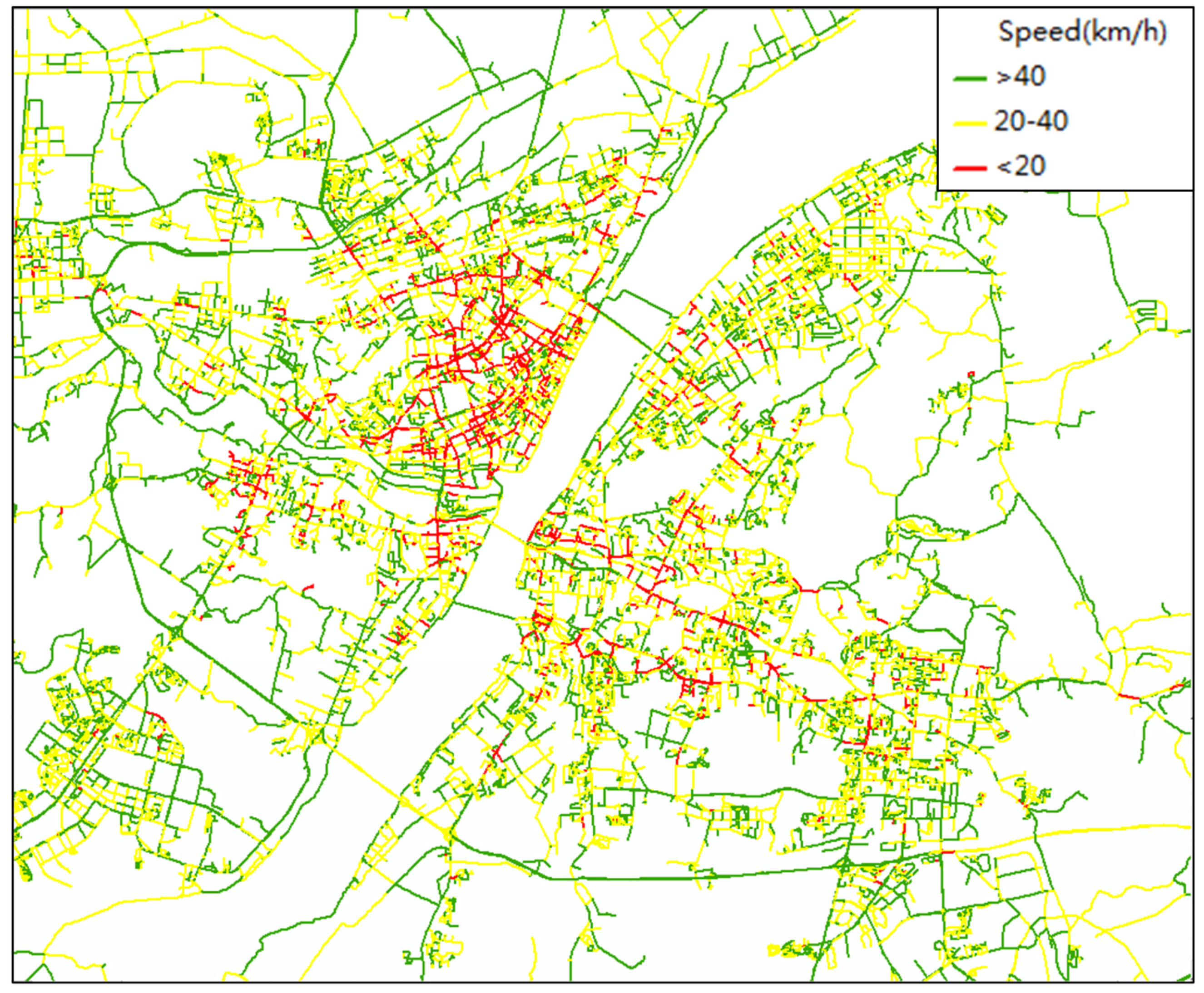
The road network in Wuhan, China, with detailed information of turn restrictions and divided/undivided roads, was adopted for this case study. As shown in Figure 4, the Wuhan road network consists of 19,306 nodes, 46,757 links and 128,965 turns. In this road network, 24,909 links are divided (i.e., 53.3% of total links) and other 21,848 links (i.e., 46.7% of total links) are undivided. The number of restricted turns is 1681, accounting for only 1.30% of total turns. To obtain link travel times of the Wuhan road network, real-world floating car data (FCD) were collected on a typical Thursday (3 September 2009). Figure 4 shows the estimated travel times during an evening peak period (6 p.m.–7 p.m.). For the detailed method of estimating these travel times, interested readers may refer to Reference [5].

Table 1. Computational performance of the four algorithms.

Travel Time Budget (min)	NTP Size	NTP-A*		NTP-BB		NTP-Dij		NTP-SN
		$\tilde{\mathit{t}}$	$\tilde{\mathit{n}}$	$\tilde{\mathit{t}}$	$\tilde{\mathit{n}}$	$\tilde{\mathit{t}}$	$\tilde{\mathit{n}}$	$\tilde{\mathit{t}}$	$\tilde{\mathit{n}}$
10	1.02%	5.75	3020	7.52	7694	629.23	743,853	71.28	101,899
20	2.96%	14.55	12,612	21.31	34,343	629.23	743,853	364.45	461,742
30	8.09%	36.02	36,300	63.16	99,646	629.23	743,853	539.69	671,069
40	14.18%	77.91	76,918	149.87	216,165	629.23	743,853	667.78	743,853
50	21.69%	143.75	137,844	293.11	368,942	629.23	743,853	667.78	743,853
60	31.27%	243.12	218,397	399.09	514,266	629.23	743,853	667.78	743,853
90	63.83%	468.05	472,997	565.62	697,992	629.23	743,853	667.78	743,853
120	88.32%	531.21	633,165	586.07	725,898	629.23	743,853	667.78	743,853
150	96.71%	593.18	702,050	600.09	736,739	629.23	743,853	667.78	743,853

$\tilde{t}$: Computational time in ms; $\tilde{n}$: Number of selected links.

reports the computational performance of all four algorithms (i.e., NTP-A*, NTP-BB, NTP-Dij and NTP-SN) in the Wuhan road network. The travel time budget (i.e., $b$) values were set from 10 to 150 min. The size of a NTP was measured by the percentage of links within the NTP over the whole network. The computational performance of all algorithms was measured by computational times ($\tilde{t}$) and the number of selected links ($\tilde{n}$). The reported computational performance was the average of 100 runs using different origin and destination (O-D) pairs. The 100 O-D pairs were randomly generated in the network and the same set of O-D pairs was used for all algorithms.

As can be seen from the table, the computational performance of the NTP-A* algorithm degraded with the increase of the travel time budget (i.e., $b$) values. For example, when $b=10$ min, the NTP-A* algorithm requires only 5.75 ms. When $b=150$ min, this computational time significantly increases to 593.18 ms. This result is obvious, due to the increase in NTP size from 1.02% to 96.71% when the $b$ values increase from 10 to 150 min. It can be observed from the table that the travel time budget parameter has no impact on the computational performance of the NTP-Dij algorithm, which consumed 629.23 ms for all $b$ values. This is because the NTP-Dij algorithm utilizes two one-to-all shortest path searches to determine the earliest departure time and latest arrival time for every network link, regardless of different $b$ values. The NTP-Dij algorithm, therefore, can have a significant computational overhead by exploring a large number of unnecessary network links, when the NTP size is small. For example, when $b=10$ min, the computational time consumed by the NTP-Dij algorithm was about 108 times (i.e., 629.23/5.75 − 1) more than that of the proposed NTP-A* algorithm.

Compared with the NTP-Dij algorithm, the NTP-SN algorithm constructs the NTP in a sub-network within the STP in the planar space, instead of the whole network. It can be seen from the table that this NTP-SN algorithm can improve the NTP construction performance when the travel time budget is very small (e.g., $b=10$ min). However, this computational improvement degrades quickly with the increase of the travel time budget (e.g., $b=30$ min). This is because the sub-network defined by the STP in the planar space was generally quite a bit larger than the actual NTP. When the travel time budget becomes large (e.g., $b>30$ min), the sub-network may reach the whole network. In this case, the sub-network generation can introduce an additional computational burden.

The proposed NTP-A* algorithm utilizes both A* and branch-and-bound techniques to improve the NTP construction performance. The effectiveness of the branch-and-bound technique was investigated through a comparison between the NTP-Dij and NTP-BB algorithms. Using the branch-and-bound technique, the NTP-BB algorithm can discard inaccessible network links of which travel times to the destination (i.e., $t_R^{id}$) (or from the origin, i.e., $t_R^{oj}$) are larger than the given travel time budget $b$. Compared with the NTP-Dij algorithm, this introduced branch-and-bound technique can significantly reduce the number of explored unnecessary links and thereby improve the NTP construction performance. For example, when $b=10$ min, the branch-and-bound technique reduced the number of selected links by 98.96% (i.e., 1 − 7694/743853). The NTP-BB algorithm, therefore, runs about 83 times faster than the NTP-Dij algorithm when $b=10$ min. Nevertheless, it can be found from the table that the effectiveness of the branch-and-bound technique degrades with the increase of travel time budget values, and becomes marginal when the size of the NTP approaches the whole network (i.e., 100%).

The effectiveness of the A* technique was examined by a comparison between the NTP-BB and NTP-A* algorithms. In the proposed NTP-A* algorithm, both the A* and branch-and-bound techniques were employed to discard the unnecessary links of which heuristic costs to the destination (i.e., $t_R^{id}+h(i)$) (or from the origin, i.e., $t_R^{oj}+h(j)$) are larger than the given travel time budget $b$. In the forward search, a heuristic function $h(j)=t_E^{jd}$ was introduced by incorporating the information of each link to the destination, while, in the backward search, the heuristic function $h(i)=t_R^{oi}$ was adopted by best using the forward search results. Compared with the NTP-BB algorithm, the introduced A* technique was effective in reducing the number of selected links by 60.75% and improved the NTP construction performance by 30.78% when $b=10$ min. The effectiveness of this A* technique became more distinct when a medium-size NTP was used. For example, when $b=40$ min, the A* technique can reduce the number of selected links by 62.63% and improve the NTP construction performance by 103.90%. Similar to the branch-and-bound technique, the effectiveness of the A* technique becomes marginal when the size of the NTP approaches that of the whole network.

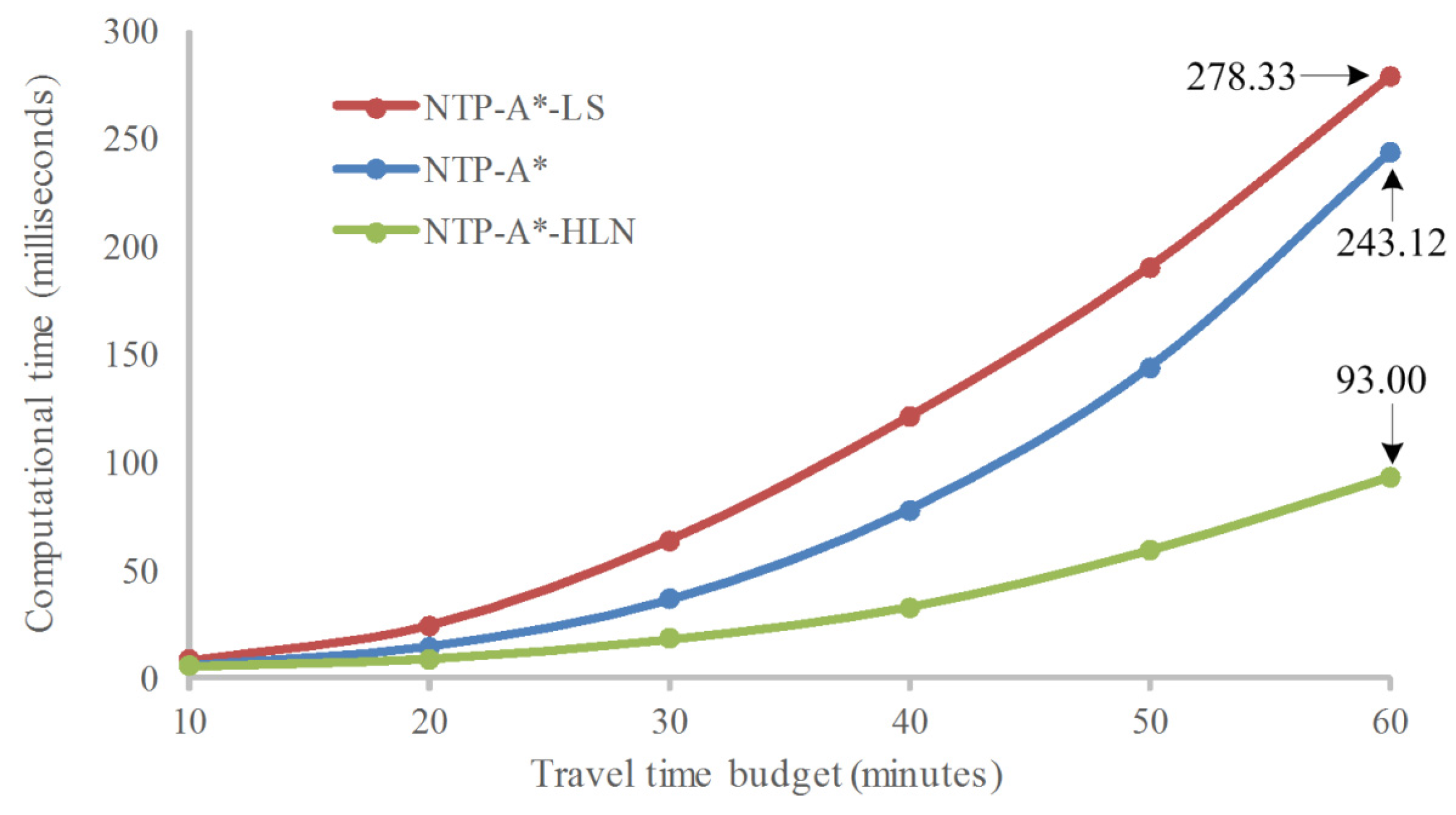
Several implementation techniques of the proposed NTP-A* algorithm were also examined. Examined first was the effectiveness of the label-correcting technique in SE implementation. Conventionally, the A*-type shortest path algorithm utilizes the label-setting technique [37,38]. For comparison, this label-setting technique was also implemented in the case study using an F-heap data structure [35] (called the NTP-A*-LS algorithm). Figure 5 illustrates the computational performance of the NTP-A* and NTP-A*-LS algorithms in the Wuhan road network. As shown in the figure, the NTP-A* algorithm using the label-correcting technique runs faster than the NTP-A*-LS algorithm using the label-setting technique. This is because the priority queue structure in the label-setting technique was computationally expensive relative to the linked-list data structure used in the label-correcting technique.

The labeling techniques for considering turn restrictions were then examined. The NTP-A* algorithm (i.e., the R-FSP and R-BSP procedures) based on the link-based labeling technique can be further enhanced by using the hybrid link-node labeling technique [36]. The hybrid link-node labeling technique adaptively uses the node-based labeling technique for unrestricted nodes without turn restrictions, and the link-based labeling technique for restricted nodes with turn restrictions. Using this hybrid link-node labeling technique, the number of paths generated, evaluated and maintained at unrestricted nodes can be reduced compared with the link-based labeling technique. Because the number of restricted nodes was small in most road networks (e.g., the Wuhan network), such a hybrid link-node labeling technique can significantly improve the computational performance of the R-BSP and R-BSP procedures. The enhanced algorithm was referred as the NTP-A*-HLN algorithm for convenience. As can be seen in the figure, the NTP-A*-HLN algorithm runs 1.99 times faster than the NTP-A* algorithm when $b=60$ min.

The computational performance of the proposed NTP-A*-HLN algorithm was further examined using four road networks with different sizes. Two existing algorithms (NTP-Dij and NTP-SN) were also examined for comparison. In addition to the Wuhan network, three other networks, the Hong Kong RTIS, the Chicago Regional and the Beijing network, were obtained from References [36,38].

Table 2. Computational times of the three NTP construction algorithms in ms.

Networks	Nodes	Links	NTP Size	NTP-A*-HLN	NTP-Dij	NTP-SN
Hong Kong RTIS	1367	3655	25.32%	2.85	8.76	9.61
Chicago Regional	12,981	39,018	7.32%	19.60	1459.42	1178.01
Wuhan network	19,306	46,757	8.09%	17.66	629.23	539.69
Beijing network	59,541	114,737	7.01%	52.01	7809.83	4891.62

gives the computational performance of the three algorithms. The reported computational performance was the average of 100 runs using randomly generated O-D pairs for each network. The travel time budget parameter was set as 30 min for all networks.

As can be seen from the table, the computational times of the three algorithms increased with the network size. The NTP-A*-HLN algorithm consumed only 2.85 ms for constructing NTPs in the Hong Kong RTIS with 3655 links. When the Beijing network was used, the size of the road network increased 30.39 times and the computational time increased by 17.24 times to 52.01 ms. Compared with the NTP-A*-HLN algorithm, the NTP-Dij algorithm degrades significantly with network size. For example, when the Beijing network was analyzed, the computational time required by the NTP-Dij algorithm increased by about 890.53 times (7809.83/8.76 − 1). This is because the NTP-Dij algorithm constructs the NTP by exploring the whole network twice. In this case, the computational time of the NTP-Dij algorithm is more sensitive to the network size. It can be observed from the table that the NTP-SN algorithm runs in a similar way to the NTP-Dij algorithm. This result confirmed that the effectiveness of constructing NTPs in the sub-networks using the STP in the planar space is marginal.

6. Conclusions

The Space-time prism is a key concept in time geography for analyzing human activity-travel behavior under various Space-time constraints. It has broad applications in numerous time-geographic studies. However, few efficient geo-computational algorithms have been developed in the literature for constructing network–time prisms (NTPs) in realistic road networks. To fill this gap, this study investigated NTP models and geo-computational algorithms. A NTP model was proposed to differentiate divided and undivided roads, and to allow individuals to make U-turns and access partial links on undivided roads. A geo-computational algorithm (called NTP-A*) was developed for efficiently constructing NTP in large-scale road networks. In the proposed algorithm, the A* and branch-and-bound techniques were employed to improve the NTP construction performance by discarding inaccessible links during two shortest path searches. The label-correcting and hybrid link-node labeling techniques were employed to improve the performance of constructing NTPs in road networks with turn restrictions. A comprehensive case study using four real road networks was carried out to demonstrate the computational advantage of the proposed NTP-A* algorithm. Experimental results showed that the proposed NTP-A* algorithm can significantly improve the existing algorithms (i.e., NTP-Dij and NTP-SN) by a factor of 100 in large-scale road networks (e.g., the Beijing network).

In this study, travel times in road networks are assumed to be static and deterministic. The proposed NTP-A* algorithm can be easily extended to construct NTPs in dynamic networks, where link travel times are varying with the time of the day. In this dynamic case, time-dependent shortest path algorithms [39] should be adopted instead of the classical Dijkstra’s algorithm. The introduced implementation techniques (including the A* and branch-and-bound techniques) are still effective for such a dynamic case. The proposed NTP-A* algorithm can also be extended to construct reliable Space-time prisms [17] in road networks with travel time uncertainties. In this stochastic case, both the A* and branch-and-bound techniques are effective, but reliable shortest path algorithms [38,40,41] should be employed for the two shortest path searches. However, the NTP construction problem becomes challenging when both dynamic and stochastic characteristics of travel times are considered. In the dynamic and stochastic networks, path travel times are found to be non-reversible [42] and cannot be generated in the reverse direction from the destination. It is an open question how to develop an efficient approach to determine the latest departure times for all accessible nodes. We leave this important extension to future research.