A Novel Evaluation Approach for Line Simplification Algorithms towards Vector Map Visualization

Abstract

Line simplification is an important method in the context of cartographic generalization, which is helpful for improving the visualization of digital vector maps. The evaluation method for the simplification algorithms is still an open issue when facing applications of vector data, including progressive transmission, web mapping, and so on. This paper proposes a novel evaluation approach for line simplification algorithms based on several factors towards vector map visualization, including the features of displays, map scales, and the ability of the human eye to distinguish pixels. In order to ensure the evaluation of the line simplification algorithms is conducted under the consistent strength of simplification, a measurement approach for the difference between an original line and its simplified one is proposed in this study, and the method of solving the appropriate simplification threshold is presented. With this method, four simplification algorithms are evaluated at five map scales using three evaluation indicators: standard deviation, compression ratio, and simplification time. The experiment and results show the evaluation approach in this study is feasible, and represents a good means in which to facilitate the application of line simplification towards progressive transmission and visualization of vector maps.

1. Introduction

The application of line simplification methods over vector maps is an important issue in the context of cartographic generalization. Line simplification has an increasingly important role in providing multi-scale vector maps. It is helpful to render a map at the scale corresponding to the zoom size of a region in digital map applications. Cartographic generalization, and in particular line simplification, is an indispensable technique when vector maps are transmitted or re-scaled over the Internet, since large datasets generally lead to longer wait times [1]. The details of a vector map can be gradually removed to generate a set of multi-scale maps by line simplification, which could help to shorten the response time in digital map applications. Thus, line simplification is one of the most important approaches to facilitate visualization of vector maps over the Internet. The approach of line simplification can also be used in improving the efficiency of zooming in and out of vector maps in WebGIS. However, the geometric strength of line simplification is an essential issue. An underpowered application of the line simplification process is likely to be unable to greatly reduce the size of vector maps. In contrast, too much line simplification may lead to the distortion of vector maps. Obviously, an appropriate amount of line simplification, which is able to make a simplified map the same as the original one in appearance, is crucial in line simplification.

Since the 1960s, many simplification algorithms have been proposed in the context of cartographic generalization. For example, the Douglas-Peucker (D-P) algorithm [2], which simplifies a line based upon vertical interval; the Reumann-Witkam (R-W) algorithm [3], which simplifies a line based upon turning angle functions [4]; the Li-Openshaw algorithm [5], which simplifies a line based upon a radius; the progressive line simplification algorithm [6], which simplifies a line based upon an area. There are other less popular algorithms besides the ones mentioned above, including the Lang algorithm [7], the Angle limited algorithm [8], the Sleeve-fitting algorithm [9], the Visvalingam-Whyatt (V-W) algorithm [10], the Circle simplification algorithm [11], and the cartographic generalization based on the B-spline snake model [12]. The goal of line simplification is to reduce the number of points by deleting some trivial points, but without destroying the essential shape of the lines in the process. The number of points being deleted is determined by an indicator called the simplification threshold in most of the simplification algorithms. The simplification threshold can be the vertical distance, radius, or area. Different simplification thresholds reflect different strengths of simplification and lead to different compression ratios and different detail-levels of vector maps. A greater strength of simplification could result in excessive generalization and cause line distortion, and lesser strength of simplification may be unable to effectively reduce the size of a vector map. Therefore, how to find the appropriate strength of simplification should be further discussed in digital vector map applications. Based on the consistent strength of simplification, a comparison of line simplification algorithms would be more meaningful.

2. Related Work

The performance evaluation of a line simplification algorithm depends on the geometric characteristics of a curve and the change of point positions [13]. Many scholars proposed various models for measuring the geometric accuracy of line simplification. Veregin [14] examined the simplification effects by quantifying the positional error of line simplification algorithms (specifically the D-P algorithm). The positional error of a line can be modelled at an aggregate level using cumulative frequency curves and their confidence limits. Then the level of simplification can be identified, and most of the vertices are eliminated in the process of attaining a specific positional accuracy standard. Shi and Cheung [15,16] evaluated the performance of nine line simplification algorithms. They used two comprehensive measurements, including displacement and shape distortion, to evaluate automated line simplification algorithms with considerations of positional accuracy and processing time. Their study shows that the D-P algorithm is more accurate, but the Lang algorithm and the Zhao–Saalfeld algorithm are more practical because they are less time-consuming. Considering influences on the spatial accuracy and the spatial relationship, Zhu and Wu [17,18] proposed a series of evaluation factors for geometric accuracy, including the sinuosity, positional error, and propagation error. Their results showed that the D-P algorithm and the Circle algorithm are better in regards to their geometric accuracy and ability to maintain geometric characteristics of lines. Chen and Zhu [19] evaluated two kinds of line simplification algorithms with considerations based upon the area-difference, bend ratio, maximal-bend-angle ratio, change-uptrend, result-coherence, and self-intersection. The D-P algorithm and Beam of Light algorithm were compared across the six different aspects, and the D-P algorithm was determined to be better than the other algorithm. In order to ensure the similarity between an original line and the simplified one, the shape similarity of vector features is another important evaluation criterion in map generalization. Liu and Luo [20] proposed a model of shape similarity for line features based on the Fourier series. The similarity degree in shape is represented as Euclidean distance. With the similarity model, six line simplification algorithms were evaluated. The D-P algorithm and Lang algorithm were determined to be better in preserving shape features. Cao and Li [21] also proposed a method to measure the shape similarity of lines. The overall shape similarity and similar precision are considered in their study. Moreover, Cao [22] proposed a model which employs considerations of weight to measure the similarity when transmitting spatial vector data progressively. In terms of a map loading and transmitting information, Deng and Fan [23] proposed a set of evaluation factors based on three information levels (the element, neighborhood, and entirety) and applied these factors in data regarding a river network. It was proven that these evaluation factors have advantages in measuring the shape change of lines. Guo and Shen [24] analyzed the time complexity of several typical line simplification algorithms and divided the line simplification algorithms into two categories: linear algorithms and nonlinear algorithms. The linear algorithms, such as the Lang algorithm, Circle algorithm, and Li-Openshaw algorithm, require less time to perform their tests. The nonlinear algorithms differ in the simplification time. However, the efficiency of the D-P algorithm is much higher than the Progressive algorithm in regards to their testing times required.

In summary, most studies above focused on measuring the geometric error between an original shape and its simplified shape. These evaluation methods first fix the compression ratio, then compare other factors (e.g., time required, difference, etc.). However, we believe the degree of the difference between an original shape and its simplified shape is determined by the strength of simplification. The higher the strength of the simplification being conducted, the bigger the expected difference between the original and the simplified version of the line(s). The comparison of line simplification algorithms with a consistent strength of simplification makes an evaluation between methods more reasonable. Moreover, the degree of a line being simplified should be determined by the application goals. For example, visualizing a vector map at the scale of 1:1,000,000 needs less strength of simplification than visualizing it at the scale of 1:250,000. Therefore, how to determine the strength of simplification at different scales should also be considered. Regarding the visualization of digital vector map, the physical parameters of displaying devices, the target map scale, and the ability of the human eye to distinguish pixels of a display are considered in order to determine the appropriate strength of line simplification. Also, the performance of line simplification algorithms should be evaluated based on a consistent strength of simplification. The next section introduces some factors that can be used in determining the strength of simplification, and is followed by an introduction of an evaluation method for line simplification. A series of experiments have been conducted based on the method, and the evaluation results are presented in Section 4. Finally, a discussion is conducted and conclusions are drawn in Section 5.

3. Methodology of the Evaluation Based on a Consistent Strength of Simplification

The detail-levels of a simplified line are closely associated with the simplification threshold of simplification algorithms. Even for the same simplification algorithm, the compression ratio and the details of vector maps vary with the different simplification thresholds. The threshold is associated with the strength of simplification. This section first introduces the simplification-related factors, which are helpful for calculating the appropriate strength of simplification at a certain scale. Then the concept of average offset distance is proposed to measure the strength of simplification. Finally, the evaluation approach of line simplification algorithms is proposed based on a consistent strength of simplification.

3.1. Simplification-Related Factors

3.1.1. Display Resolution (H_res × V_res)

Display resolution means the number of total pixels in each of the dimensions. Typically, a display device has a horizontal dimension and a vertical dimension, denoted by H_res × V_res, respectively, with the units in pixels. The higher the resolution a display device has, the finer effect it has. Thus, displays with higher resolutions will present bigger difference in appearance between an original line and its simplified version. In this situation, there might be a need for a less strong simplification in order to reduce the differences in appearance. Therefore, it is necessary to consider the display resolution when determining the appropriate threshold of simplification algorithms.

3.1.2. Display Size (D_scr)

Display size means the physical size of a display screen. It is commonly measured by the diagonal size of display devices, denoted as D_scr in inches. With the same display resolution, bigger display screens have bigger pixel sizes.

3.1.3. Pixels per Inch (PPI)

Pixels per inch (PPI) is an indicator to measure the pixel density of display devices. The PPI can be calculated with display size in inches and display resolution. The formula on PPI is as follows:

$$\mathrm{PPI}=\frac{\sqrt{{H_{res}}^2+{V_{res}}^2}}{D_{scr}}$$

(1)

where H_res is the horizontal resolution in pixels, V_res is the vertical resolution in pixels, and D_scr is the diagonal size in inches. With higher PPI, images or graphs shown in a display would appear clearer. The physical length of a pixel, denoted by D_pixel, is calculated based on the PPI. The spatial resolution, which leads to different strength of simplification, is determined by the pixel length. The pixel length can be calculated as follows:

$$D_{pixel}=\frac{1}{\mathrm{PPI}}\left(\mathrm{inches}\right)=\frac{0.0254}{\mathrm{PPI}}\left(\mathrm{m}\right)=\frac{25.4}{\mathrm{PPI}}\left(\mathrm{mm}\right)$$

(2)

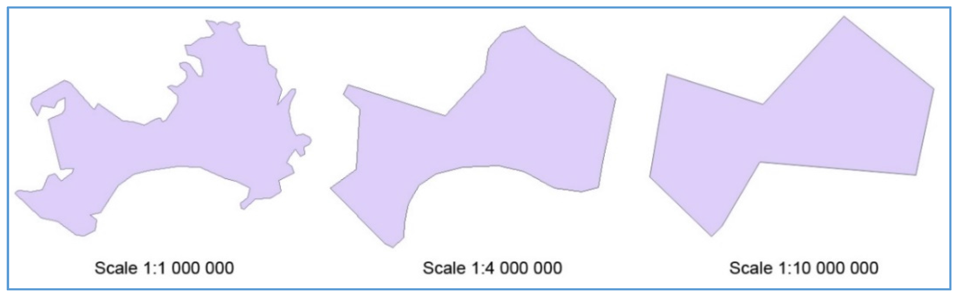
3.1.4. Map Scale (Scale)

Map scale means the ratio of a distance on the map corresponding to the distance on the ground. The details of vector data vary with the map scale. Maps in different scales reflect different strengths of simplification, as illustrated in Figure 1. The map scale has a quantitative relationship with PPI and spatial resolution, which will be discussed below. Usually, a map scale is the initial condition in practical applications. Thus, the map scale defines the goal of simplification.

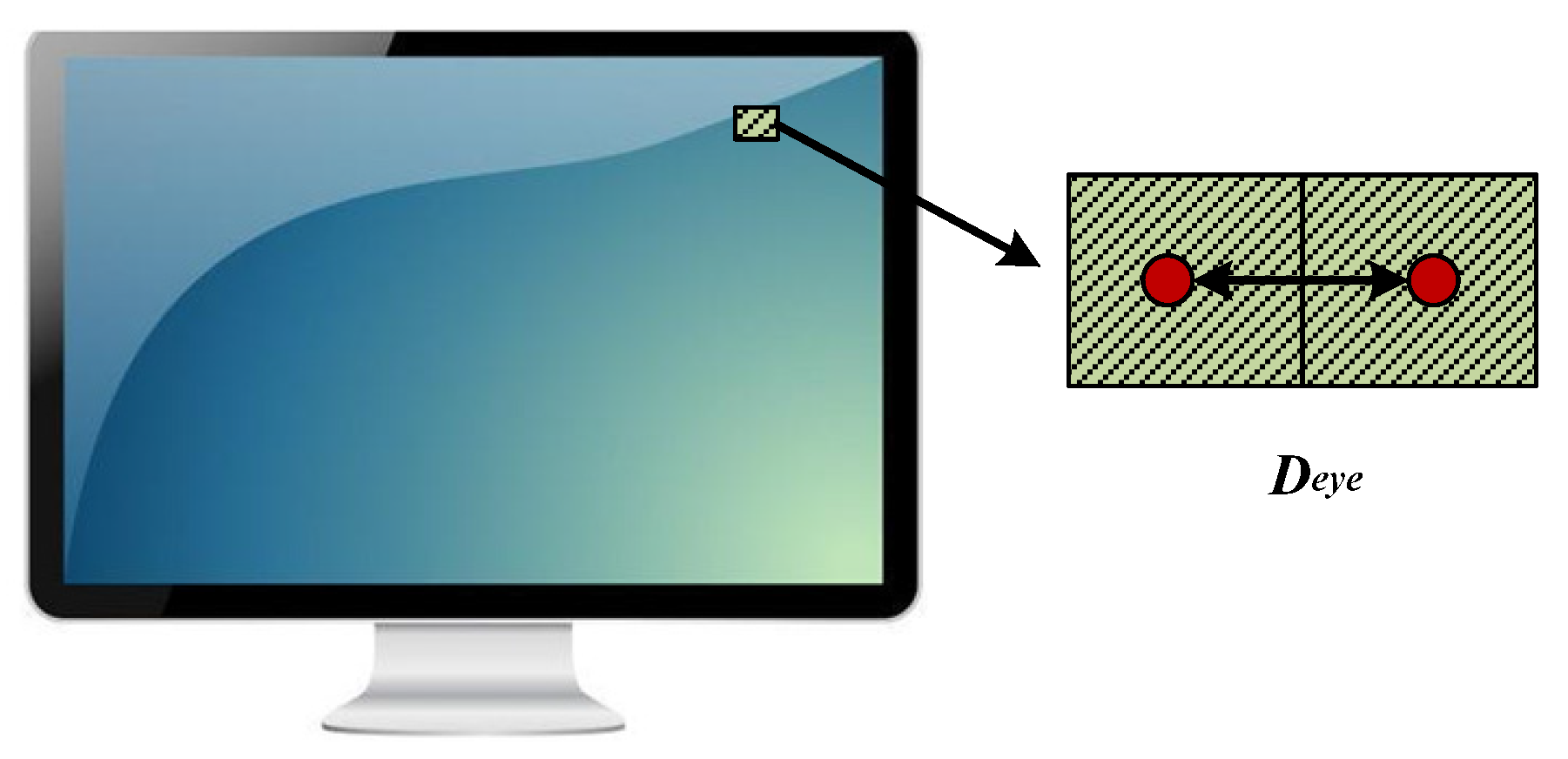
3.1.5. Spatial Resolution of Pixels (SR_pixel)

Spatial resolution, or ground resolution, describes the actual distance of pixels. It can reflect the capability in distinguishing details of vector features. The spatial resolution of pixels is associated with the map scale (Scale) and physical length of pixels (D_pixel). The quantitative relation among them is as follows:

$$\mathrm{S}{R}_{pixel}=\frac{D_{pixel}}{\mathrm{Scale}}=\frac{0.0254}{\mathrm{PPI}\times \mathrm{Scale}}\left(\mathrm{m}\right)= \frac{0.0254\times D_{scr}}{\mathrm{Scale}\times \sqrt{{H_{res}}^2+{V_{res}}^2}}\left(\mathrm{m}\right)$$

(3)

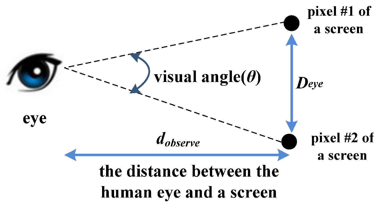
3.1.6. Resolution of the Human Eye

Visual perception of the human eye is also one of the essential aspects for consideration in the visualization of digital vector maps. The minimum angle that the unaided human eye can distinguish is about 1 min of arc in terms of Rayleigh’s Criterion. Thus, the human eye probably fails to distinguish two objects which get too close in distance. The simple model of a human vision system is illustrated in Figure 2.

The minimum distance of the human eye to distinguish, denoted by D_eye in Figure 2, can be calculated with the minimum distinguishing angle (θ) and the distance between the eyes and a screen (d_observe) as follows:

$$D_{eye}=2\times d_{observe}\times \tan \frac{\theta }{2}=2\times \tan \frac{1}{120}\times d_{observe}=0.000291\times d_{observe}\left(\mathrm{mm}\right)$$

(4)

when the $d_{observe}$ is denoted as 600 (mm), which is the applied standard, D_eye is going to be 0.1746 (mm).

Since pixels are the smallest unit of a screen, the number of pixels is used to replace the D_eye in practical experiments. The number of pixels (N_eye) corresponding to the D_eye is calculated as follows:

$$N_{eye}=\lceil \frac{D_{eye}}{D_{pixel}}\rceil =\lceil \frac{0.000291\times d_{observe}\times \mathrm{PPI}}{25.4}\rceil =\lceil \frac{0.1746\times \mathrm{PPI}}{25.4}\rceil$$

(5)

where the symbol of ⌈$\frac{D_{eye}}{D_{pixel}}$⌉ means rounding up N_eye to the minimum integer greater than $\frac{D_{eye}}{D_{pixel}}$, and $D_{pixel}$ is the physical length of pixels in millimeters. Formula (5) shows the minimum number of pixels that the human eye can distinguish. With retina screens in which the PPI normally is more than 200, N_eye would be 2, as shown in Figure 3. With regular screens in which the PPI is less than 145, N_eye would be 1. The above results are based on people who keep 600 mm away from a screen.

3.2. Appropriate Strength of Line Simplification

With the above simplification-related factors, we further propose the threshold of the ground distance (D_ground) on the basis of considering N_eye in order to find the appropriate strength of simplification. (D_ground) is defined by the following formula:

$$D_{ground}={SR}_{pixel}\times N_{eye}=\frac{0.0254}{\mathrm{PPI}\times \mathrm{Scale}}\times N_{eye}\left(\mathrm{m}\right)$$

(6)

where the SR_pixel is the spatial resolution, and N_eye is the minimum number of pixels that the human eye can distinguish. The D_ground represents the maximum offset distance between an original line and its simplified equivalent. Keeping the offset distance of simplified lines within D_ground could ensure that they remain similar to the original ones, overall. Thus, D_ground is used in order to limit the strength of simplification applied in this study.

The offset distance of a line being simplified can be illustrated in Figure 4. The original polyline is denoted by the green solid lines and its simplified polyline is denoted by the red dotted line; d_i denotes the offset distance. For a whole line, even a vector map, the concept of average offset distance is proposed in our study, which is denoted by $\overline{d}$ as follows:

$$\overline{d}=\frac{{{\displaystyle \sum }}_1^n{d}_i}{n}$$

(7)

where d_i is the offset distance of the i^th line segment, and n is the number of line segments. With the average offset distance, the difference between an original line and its simplified version is quantified. In other words, the average offset distance makes the difference between them measurable.

Towards the visualization of a vector map, the goal of simplification is that simplified lines have no apparent difference with original ones in appearance. When the average offset distance is equal to D_ground at a certain map scale, which means that the simplification strength of the line just reaches the limitation of the difference that is able to be distinguished by the human eye, the removed points reach the maximum at the same time. Therefore, the simplification threshold corresponding to the average offset distance is the appropriate strength of line simplification.

3.3. Evaluation Approach Based on a Consistent Strength of Simplification

In this study, four representative simplification algorithms are evaluated based on a consistent strength of simplification. They are D-P algorithm, Progressive algorithm, Angle algorithm, and Circle algorithm. The D-P algorithm is an iterative algorithm that is based upon considering vertical distance. Vertical distances between each of the points and the line connected with the starting point and ending point are calculated first. The points are removed when their vertical distances are less than the given simplification threshold. Similarly, the Progressive algorithm is an iterative algorithm that is based upon considering area. It traverses each of the points apart from the starting and ending points. The simplification threshold of the Angle algorithm is based upon considering angles. A point is removed if the angle of this point and its adjacent two points is less than the given simplification threshold. The idea of the Circle algorithm is as follows: starting with one of the sides of a line, the algorithm makes circles with each of their centers located at each of the points of a line. The radius of these circles is the threshold of simplification. The next adjacent point is removed if it is located inside a circle. Otherwise, the point is reserved.

According to Section 3.2, if the average offset distance is less than or equal to the D_ground, the difference between the original line and its simplified one is hard to perceive by the human eye. The average offset distance in this situation is the goal of line simplification at the corresponding map scale. In order to get the average offset distance which is closest to D_ground, we propose a method of successive approximation to find the appropriate simplification threshold. The procedures are as follows:

Step 1: Initialize a series of simplification thresholds: $G=\{G_1,G_2,\dots ,G_i,\dots ,G_n\}$, and the adjacent thresholds are set at equal intervals, namely, $G_2-G_1=G_3-G_2=\dots =G_n-G_{n-1}$. The initial number of elements of the G is equal to the number of line segments. G₁, which is the minimum value of the G set, is the starting element. G_n, which is the maximum value of the G set, is the ending element.

Step 2: Get the collection of simplified results for each of the thresholds: G_i ($G_i\in G$).

Step 3: Calculate the average offset distance between an original line and its simplified one, respectively, and get the collection of the average offset distance: $\overline{d}=\{\overline{d_1},\overline{d_2},\dots ,\overline{d_i},\dots ,\overline{d_n}\}$. Each offset distance ($\overline{d_i}$) of line segments can be calculated with the vertical distance between the removed point and the simplified line segment.

Step 4: Find the $\overline{d_t}$ nearest to D_ground among the elements of $\overline{d}$. In the meantime, find the simplification threshold $G_t$ corresponding to $\overline{d_t}$.

Step 5: Repeat Step 1~5 recursively in $[G_t,G_{t+1}]$ until G_t is approximately equal to G_t+1, which means that the average offset distance under the simplification threshold $G_t$ equals or very nearly approaches D_ground.

The above steps are not only helpful for finding the appropriate simplification threshold $G_t,$ but also helpful for evaluating the simplification algorithms conducted under a consistent strength of simplification.

4. Experiment and Results

Based on the above thought and method, the simplification experiment of four typical algorithms was conducted with five different map scales. This section introduces the data and the conditions which the experiment requires, followed by the simplification results and the evaluation results.

4.1. Experimental Data and Enviroment

The experiment data was 1:1,000,000 railway data of China from the 1980s, which has 504 polyline features. The number of point coordinates of the data is 7296. Four algorithms: D-P algorithm, Progressive algorithm, Angle algorithm, and Circle algorithm were implemented in Python language with open source GDAL (Geospatial Data Abstraction Library) library. Five map scales were selected in the experiment. They were 1:2,500,000, 1:5,000,000, 1:10,000,000, 1:25,000,000, and 1:50,000,000. The size of computer display was 19 inches with $1440\times 900 \mathrm{screen} \mathrm{resolution}$. With Formulas (1) and (2), the PPI of the screen was 90 and the physical length of pixel $\left(D_{pixel}\right)$ was 0.2822 mm. We defined the distance between the human eye and the screen as being 600 mm in the experiment. Thus, the minimum distance that the human eye was able to distinguish was 0.1746 mm in terms of Formula (4), and the corresponding number of pixels was 1 in terms of Formula (5). Therefore, we obtained five ground distances (D_ground), as shown in

Table 1. The distances corresponding to minimum resolvable pixels.

Scale *	1:2.5 M	1:5 M	1:10 M	1:25 M	1:50 M
Dground (meters)	705	1411	2822	7055	14,111

* 1 M = 1,000,000.

, which are respectively associated with the five designated map scales.

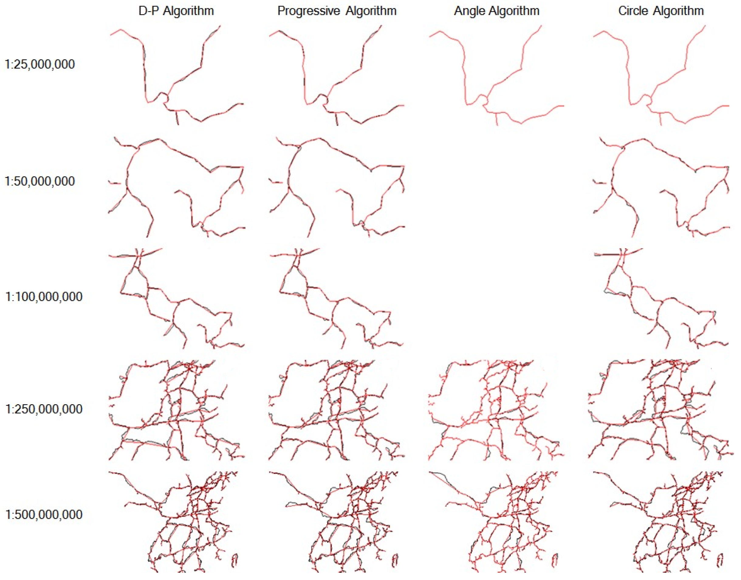
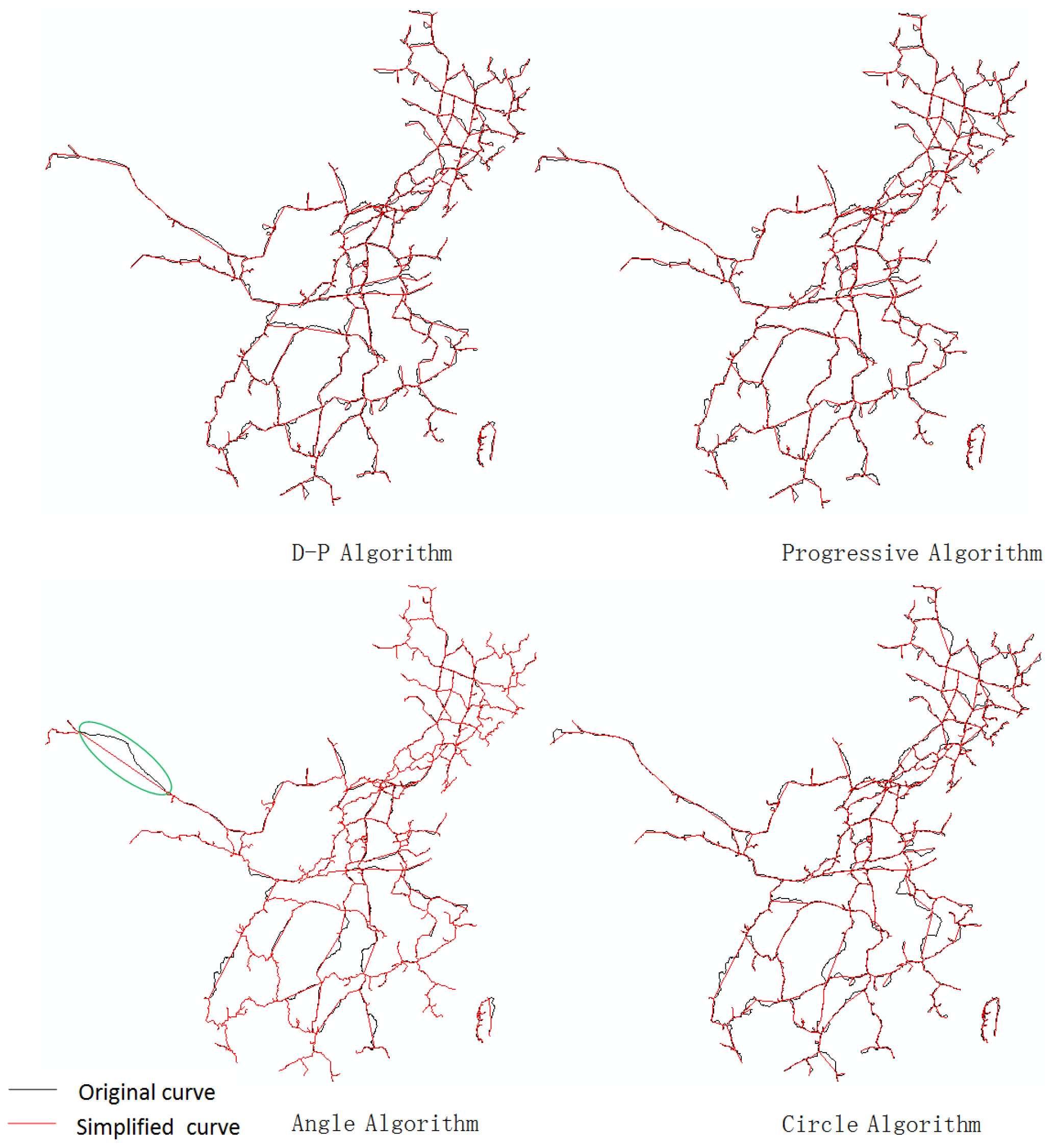
4.2. Results of the Simplification

The threshold types of the four simplification algorithms are vertical distance, area, angle, and radius. We obtained five thresholds for each of the simplification algorithms with the five map scales, as shown in

Table 2. The simplification threshold of the four simplification algorithms.

	Scale *	1:2.5 M	1:5 M	1:10 M	1:25 M	1:50 M
Algorithm (Threshold)
D-P (vertical distance)		1736 m	4215 m	9543 m	33918 m	79572 m
Progressive(area)		17 km2	73 km2	295.198 km2	2774 km2	15,373.778 km2
Angle (degree)		2.21°	--	--	4.53°	5.62°
Circle (radius)		3.441	0.5547	0.2197	0.06091	0.0431

D-P: Douglas-Peucker algorithm; * 1 M = 1,000,000.

. We did not get accurate threshold values for the Angle algorithms at 1:5 M and 1:10 M map scale. With further analysis based on the average offset distance, a curve of the average offset distance varying with threshold is shown in Figure 5. According to Table 1, the values of D_ground at 1:5 M and 1:10 M are 1411 m and 2822 m, respectively, but the jump from 1265 m to 4714 m in average offset distance happened between 2.8 degrees and 3.0 degrees, respectively, which resulted in the failure of us getting the appropriate threshold values at the 1:5 M and 1:10 M scale. This might be raised by the experimental data, in which the angle of most triangles enclosed by adjacent points was around 2.8 degree.

The results of the railway data of China having been simplified are shown in Figure 6. The black lines are the original lines and the red lines are the simplified lines. The figure shows that most of simplified lines fit the original ones very well.

4.3. Results of the Evaluation

In order to compare the performance of the four algorithms, three indicators: standard deviation, compression ratio, and simplification time were selected for evaluating the line algorithms.

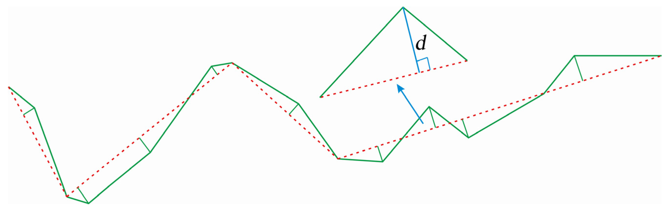
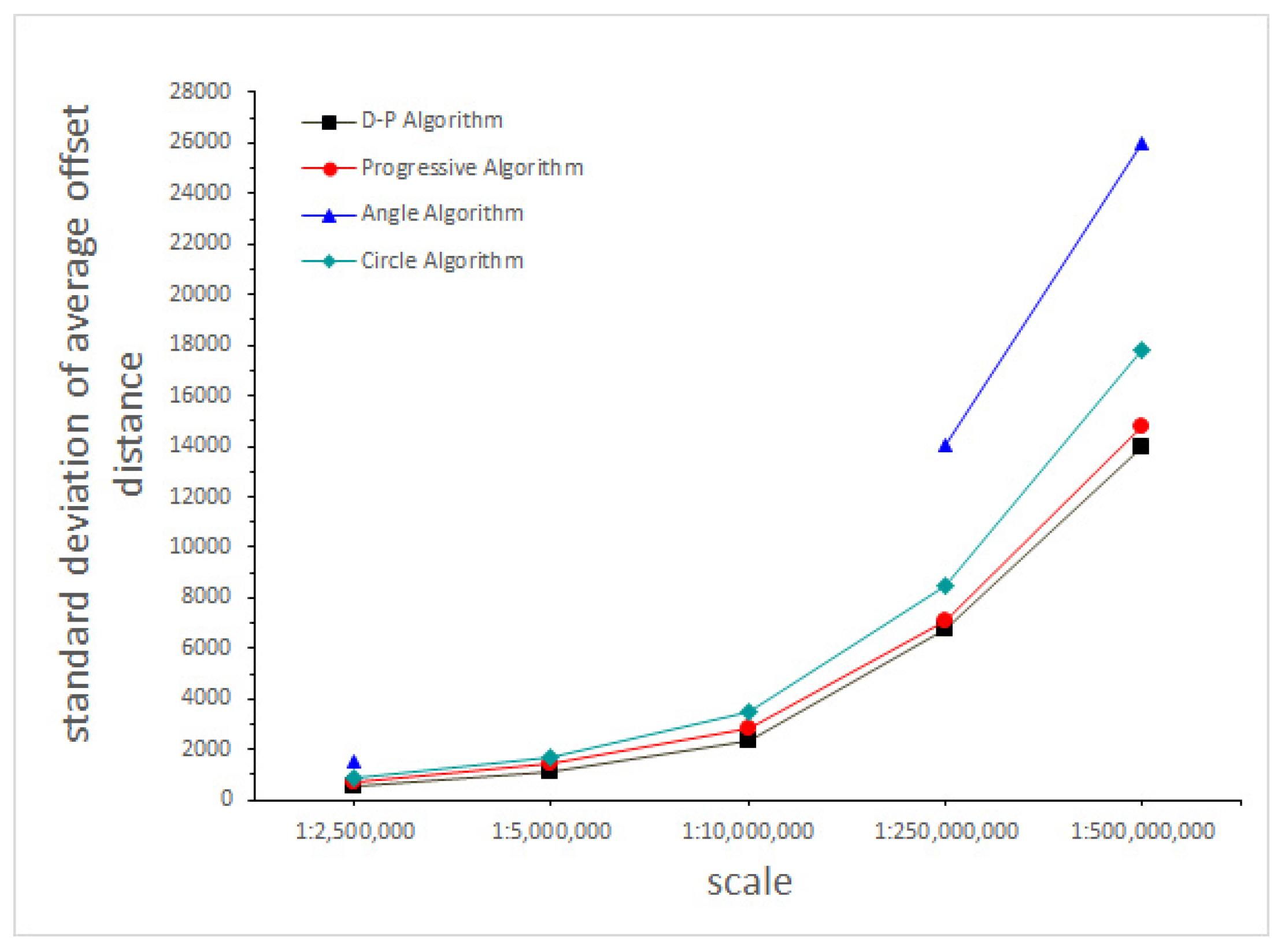
4.3.1. Standard Deviation of Average Offset Distance

Figure 7 shows the result of standard deviation of average offset distance. The D-P algorithm, Progressive algorithm, and Circle algorithm perform well on the standard deviation of average offset distance. They do not have obvious differences when compared with the value of D_ground in Table 1. The standard deviation of average offset distance for the D-P algorithm is lowest. The standard deviation of average offset distance on the Angle algorithm is the highest, especially when the map scale is getting small. It reveals that there are some simplified line segments which become far away from the original ones when using the Angle algorithm, as shown in Figure 8 with the green line circled.

4.3.2. Compression Ratio

The compression ratio of the four simplification algorithms is shown in Figure 9. The compression ratio goes up as the map scale gets smaller. The D-P algorithm and Progressive algorithm have the same capability in compression ratio. Also, they are better than the other two algorithms, with up to approximately 55% to 85% higher compression ratios. Figure 9 also shows that the Circle algorithm is low in compression ratio when the map scale is 1:2.5 M, and the Angle algorithm does not have a high compression ratio regardless of the map scale.

4.3.3. Simplification Time

Figure 10 shows the result of the simplification time for the four algorithms. Obviously, the Progressive algorithm takes longer time. The simplification time of the D-P algorithm experiences some minor change with different map scales. The Angle algorithm and Circle algorithm require similar simplification times, and the simplification time of these algorithms are shortest among the four algorithms. In addition, the simplification times of the Angle algorithm and Circle algorithm vary only a little with different map scales.

5. Discussion and Conclusions

Simplification threshold, which determines the number of removed points, is the essential parameter of line simplification algorithms. However, studies on how to determine the appropriate simplification threshold are very limited. With the aim of specifically considering the visualization of digital vector maps, several factors, including the features of a display, map scale, and human eye, were proposed to determine the appropriate simplification threshold, and a method of successive approximation based on these factors was illustrated in this study. More importantly, the method presented here is helpful for ensuring that the simplification is conducted with a consistent strength of simplification, and the evaluation based on a consistent strength of simplification makes the evaluation of simplification more reasonable. The evaluation based on considering a consistent simplification strength demonstrated the following conclusions:

(1) The D-P algorithm and Progressive algorithm are better at maintaining the shape of a line, and both of them have better compression ratios at all map scales in the experiment. The Progressive algorithm requires longer simplification time when compared with the D-P algorithm. The good performance in maintaining the shape confirms that both of these two algorithms are good at retaining the overall characteristics of lines. The difference of the two algorithms in the simplification time can be verified by time complexity. The time complexity of the D-P algorithm is $\mathrm{O}\left(\mathrm{n}\log n\right)$, and the time complexity of the Progressive algorithm is $\mathrm{O}(n^2)$.

(2) The Angle algorithm has higher time efficiency. However, it is not a stable algorithm. It is possible that the simplification threshold may not be suitable for some map scales. In addition, the compression ratio of this algorithm is relatively lower than the other algorithms. In rare situations, it is possible for considerable distortion to occur.

(3) The Circle algorithm has higher time efficiency as well, and its time complexity is $\mathrm{O}\left(\mathrm{n}\log n\right)$. The simplification effect of this algorithm is quite good. It can be seen that the Circle algorithm performs better at small map scales and that it has low compression ratios at large map scales. Since the radius of circles get progressively smaller at larger map scales, the probability of points being inside the circles is going to be low at larger map scales. Thus, there will be few points removed at larger map scales, and the compression ratio will not be satisfied.

Compared with other evaluation methods, although some evaluation results in this study are the same as others, the experiment details in this study are different. This experiment ensured that all four line algorithms were conducted based on a consistent strength of simplification. Some other evaluation studies concluded that the D-P algorithm performs better, but those conclusions are based on criteria that are different than this study. Therefore, this study is an effective complement of other previously considered evaluation approaches. In addition, this study puts more focus on the novel evaluation approach, and does not evaluate all common simplification algorithms. We selected four simplification algorithms in order to demonstrate how the evaluation approach works. Currently, the proposed method in determining the simplification threshold is an iterative algorithm in essence, which is a little bit time-consuming. For future work, we will consider improving the efficiency of our method in finding the appropriate simplification threshold. The parallel techniques can first be employed in simplifying multiple line features simultaneously. When dealing with each of the single lines, more effective algorithms for iterative computations can be investigated and applied in solving the simplification threshold since the computing process in our method is somewhat of an iterative process.

References

1. Jones, C.B.; Mark Ware, J. Map generalization in the web age. Int. J. Geogr. Inf. Sci. 2005, 19, 859–870. [Google Scholar] [CrossRef]
2. Douglas, D.H.; Peucker, T.K. Algorithms for the reduction of the number of points required to represent a digitized line or its caricature. Cartogr. Int. J. Geogr. Inf. Geovis. 1973, 10, 112–122. [Google Scholar] [CrossRef]
3. Reumann, K.; Witkam, A.P.M. Optimizing curve segmentation in computer graphics. In Proceedings of the International Computing Symposium, Davos, Switzerland, 4–7 September 1973; pp. 467–472.
4. Rangayyan, R.M.; Guliato, D.; de Carvalho, J.D.; Santiago, S. Polygonal approximation of contours based on the turning angle function. J. Electron. Imaging 2008, 17, 023016. [Google Scholar]
5. Li, Z.; Openshaw, S. A natural principle for the objective generalization of digital maps. Cartogr. Geogr. Inf. Syst. 1993, 20, 19–29. [Google Scholar] [CrossRef]
6. Qingsheng, G.; Brandenberger, C.; Hurni, L. A progressive line simplification algorithm. Geo-Spat. Inf. Sci. 2002, 5, 41–45. [Google Scholar] [CrossRef]
7. Lang, T. Rules for robot draughtsmen. Geogr. Mag. 1969, 42, 50–51. [Google Scholar]
8. McMaster, R.B. Automated line generalization. Cartogr. Int. J. Geogr. Inf. Geovis. 1987, 24, 74–111. [Google Scholar] [CrossRef]
9. Zhao, Z.; Saalfeld, A. Linear-time sleeve-fitting polyline simplification algorithms. In Proceedings of the Annual Convention and Exposition Technical Papers (AutoCarto), Seattle, WA, USA, 7–10 April 1997; Volume 13, pp. 214–223.
10. Visvalingam, M.; Whyatt, J.D. Line generalisation by repeated elimination of points. Cartogr. J. 1993, 30, 46–51. [Google Scholar] [CrossRef]
11. Qian, H.; Liu, Y.; Zhang, L.; Niu, H. Map generalization algorithm research based on circle characters. Hydrogr. Surv. Charting 2005, 25, 14–17. (In Chinese) [Google Scholar]
12. Guilbert, E.; Saux, E. Cartographic generalisation of lines based on a B-spline snake model. Int. J. Geogr. Inf. Sci. 2008, 22, 847–870. [Google Scholar] [CrossRef]
13. Balboa, J.L.G.; López, F.J.A. Sinuosity pattern recognition of road features for segmentation purposes in cartographic generalization. Pattern Recognit. 2009, 42, 2150–2159. [Google Scholar] [CrossRef]
14. Veregin, H. Quantifying positional error induced by line simplification. Int. J. Geogr. Inf. Sci. 2000, 14, 113–130. [Google Scholar] [CrossRef]
15. Cheung, C.K.; Shi, W. Estimation of the positional uncertainty in line simplification in GIS. Cartogr. J. 2004, 41, 37–45. [Google Scholar] [CrossRef]
16. Shi, W.; Cheung, C.K. Performance evaluation of line simplification algorithms for vector generalization. Cartogr. J. 2006, 43, 27–44. [Google Scholar] [CrossRef]
17. Zhu, K.P.; Wu, F. Error propagation model of linear features’ simplification algorithms. Geomat. Inf. Sci. Wuhan Univ. 2007, 32, 932–935. (In Chinese) [Google Scholar]
18. Wu, F.; Zhu, K.P. Geometric accuracy assessment of linear features’ simplification algorithms. Geomat. Inf. Sci. Wuhan Univ. 2008, 33, 600–603. (In Chinese) [Google Scholar]
19. Chen, B.; Zhu, K.P.; Xue, B.X. Analysis and assessment of linear features simplification algorithms. J. Zhengzhou Inst. Surv. Mapp. 2007, 24, 121–124. (In Chinese) [Google Scholar]
20. Liu, P.C.; Luo, J.; Ai, T.H.; Li, C. Line features comprehensive evaluation model based on shape similarity. Geomat. Inf. Sci. Wuhan Univ. 2012, 37, 114–117. (In Chinese) [Google Scholar]
21. Cao, Z.Z.; Li, M.C.; Xu, J.H. The measure of graphic similarity in cross-scaling. Sci. Surv. Mapp. 2013, 38, 131–132. (In Chinese) [Google Scholar]
22. Cao, Z.Z. A similarity measurement model for multi-resolution transmission of curve datasets over the internet. Geomat. Inf. Sci. Wuhan Univ. 2014, 39, 1257–1260. (In Chinese) [Google Scholar]
23. Deng, M.; Fan, Z.D.; Liu, H.M. Performance evaluation of line simplification algorithms based on hierarchical information content. Acta Geod. Cartogr. Sin. 2013, 42, 767–773. (In Chinese) [Google Scholar]
24. Guo, L.S.; Shen, J.; Zhu, W. The time complexity of linear features simplification algorithms. J. Zhengzhou Inst. Surv. Mapp. 2012, 29, 226–230. (In Chinese) [Google Scholar]
Figure 1. The representation of vector data at different scales.
Ijgi 05 00223 g001
Figure 2. The simple model of the human eye.
Ijgi 05 00223 g002
Figure 3. The minimum number of pixels that the human eye can distinguish.
Ijgi 05 00223 g003
Figure 4. The average offset distance of a polyline.
Ijgi 05 00223 g004
Figure 5. The curve of the average offset distances varying with simplification thresholds.
Ijgi 05 00223 g005
Figure 6. The simplification results of four algorithms.
Ijgi 05 00223 g006
Figure 7. The standard deviation of average offset distance of the four simplification algorithms.
Ijgi 05 00223 g007
Figure 8. The simplification results of four algorithms at the 1:25,000,000 map scale.
Ijgi 05 00223 g008
Figure 9. The compression ratio of the four simplification algorithms.
Ijgi 05 00223 g009
Figure 10. The simplification times required by the four simplification algorithms.
Ijgi 05 00223 g010