Characterizing Traffic Conditions from the Perspective of Spatial-Temporal Heterogeneity

Abstract

Traffic conditions are usually characterized from the perspective of travel time or the average vehicle speed in the field of transportation, reflecting the congestion degree of a road network. This article provides a method from a new perspective to characterize traffic conditions; the perspective is based on the heterogeneity of vehicle speeds. A novel measurement, the ratio of areas (RA) in a rank-size plot, is included in the proposed method to capture the heterogeneity. The proposed method can be performed from the perspective of both spatial heterogeneity and temporal heterogeneity, being able to characterize traffic conditions of not only a road network but also a single road. Compared with methods from the perspective of travel time, the proposed method can characterize traffic conditions at a higher frequency. Compared to methods from the perspective of the average vehicle speed, the proposed method takes account of the heterogeneity of vehicle speeds. The effectiveness of the proposed method has been demonstrated with real-life traffic data of Shenzhen (a coastal urban city in China), and the advantage of the proposed RA has been verified by comparisons to similar measurements such as the ht-index and the CRG index.

1. Introduction

Traffic condition refers to the volume of network traffic and its spatial distribution across the traffic network [1]. It is simply divided into levels such as light, medium, and heavy, reflecting the degree of congestion. This condition has become a major concern for a large number of cities all over the world [2,3], as there are more and more traffic congestions and these congestions have a huge cost to society [4,5,6,7]. To manage and control the congested traffic, many cities are taking a range of actions. One important action is to monitor their traffic conditions around the clock. For example, traffic conditions of San Francisco are monitored all day and night (see the website http://traffic.511.org/).

The second step after monitoring the traffic is to characterize its conditions, or the degree of congestion. In addition to simple descriptions such as light and heavy, there are mainly two basic perspectives to characterize traffic conditions in the field of transportation, i.e., travel time and vehicle speeds. For the first perspective, the travel time index has been usually used by many institutes such as the Texas A&M Transportation Institute (see its annual urban mobility reports). This index is a ratio of the travel time required during peak traffic periods to the normal travel time [8]. For the second perspective, an average of vehicle speeds is generally used to characterize the traffic condition of a traffic network. A typical example is the index developed by the Beijing Municipal Commission of Transport (http://www.bjjtw.gov.cn/), who publishes the average vehicle speed of Beijing as an indicator of congestions on its website at a frequency of five minutes. Apart from the two basic perspectives, there are other methods measuring traffic conditions from perspectives such as the capacity adequacy; for example, an index termed ACCESS developed by Boarnet, et al. [9]. However, except the average vehicle speed, most methods are not able to characterize traffic conditions in real time. Furthermore, most methods including those based on vehicle speeds pay too much attention to average values, ignoring the spatial heterogeneity of traffic conditions.

Spatial heterogeneity refers to the tendency for the distribution of geographical features or the process of geographical phenomena to be statistically non-stationary [10,11]. This non-stationary phenomenon can be characterized by a heavy-tailed distribution in general [12]. As the distribution of light-, medium-, and heavy-traffic roads can be regarded as a kind of spatial heterogeneity, traffic conditions can also be characterized from the perspective of spatial heterogeneity. This has been demonstrated by a pioneering work conducted by Gao, et al. [13] on measuring the traffic flow of San Francisco Bay Area based on the proposed index, which is termed the cumulative rate of growth (i.e., CRG index). The CRG index was obtained based on ratios such as the number of light-traffic roads to the number of heavy-traffic roads, successfully characterizing the heavy-tailed distribution of roads with different traffic conditions (another similar index is the ht-index [14]). However, the work is limited by its input; the traffic condition was characterized based on a series of raster images showing the traffic flow, rather than raw data such as vehicle speeds or traffic volumes monitored by the government.

This work was inspired by the pioneering work on characterizing spatial heterogeneity [15,16,17,18,19,20], and extended the work conducted by [13]. The contribution of this work is threefold. First, the raw data of monitored traffic was utilized instead of products such as raster images, and methods to process the raw data were put forward. Second, a novel index was proposed to characterize traffic conditions of a road network from the perspective of spatial heterogeneity, because we found the CRG index proposed in the pioneering work was ineffective when dealing with the raw data. Third, a method to characterize the traffic condition of a single road was put forward; the method was based on temporal heterogeneity.

The remainder of this paper is structured as follows. Section 2 describes the raw data used in this work and the procedure of processing the raw data. Section 3 introduces the methodology to characterize traffic conditions from the perspective of spatial-temporal heterogeneity, and the characterized traffic conditions are presented in Section 4. Section 5 further discusses the proposed methodology. Finally, Section 6 draws conclusions.

2. Data and Data Processing

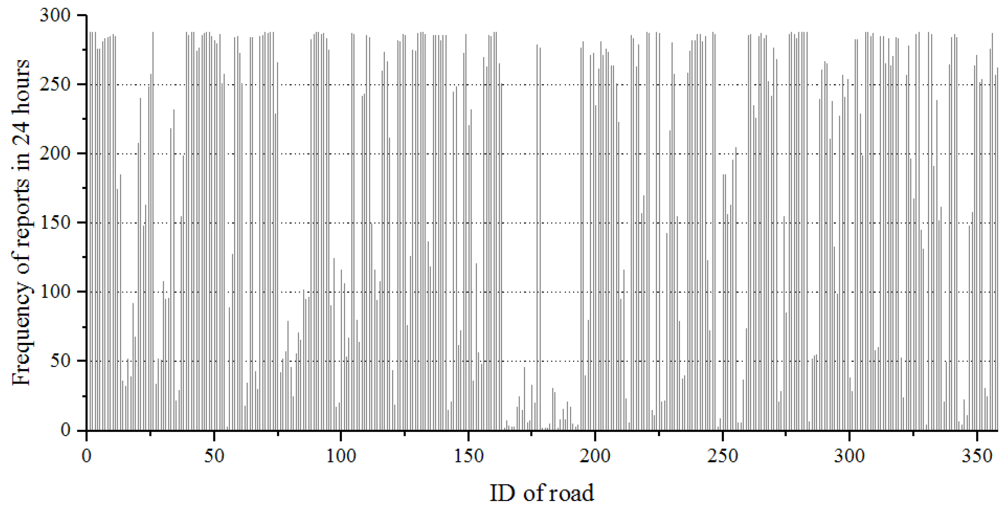
The data used in this study are the raw data produced by the traffic monitoring system of Shenzhen, a coastal urban city in southern China. The raw data are produced as a file every five minutes. Each file contains real-time vehicle speeds on all monitored roads at a specific moment. Main roads in Shenzhen are monitored in two directions, and they are regarded as two independent roads in this study. The raw data of Shenzhen can be considered as representative of monitored traffic data of most cities because of its form of vehicle speeds, but these data are not entirely satisfactory because the vehicle speeds are reported at different frequencies.

Frequencies of reports vary largely for different monitored roads. There are in total 358 roads in Shenzhen that are monitored. For a set of raw data in 24 h, it contains 288 files reporting vehicle speeds in every five minutes. As roads are monitored at different frequencies, not all files contain information for all the 358 monitored roads at that moment. In other words, though the traffic monitoring system produces 288 files in a day, a single road may not report 288 vehicle speeds during this period. Figure 1 shows the reporting frequencies of the 358 roads in a one-day period (from 20:20, 14 October 2015 to 20:15, 15 October 2015).

The varying report frequency largely affects the characterization of traffic conditions because of two reasons. First, it makes characterized traffic conditions for two moments (or, from two files) incomparable, because the numbers of vehicle speeds reported at the two moments are usually different. In other words, traffic conditions for the two moments are, in fact, characterized for two different traffic networks, so the two conditions are not comparable. Second, it makes the method of the pioneering work less suitable in characterizing the heterogeneity, since the varying number of vehicle speeds may introduce significant errors in the degree of heterogeneity characterized by the ht-index or the CRG-index.

To cope with the problem of the varying frequency, a two-step method was developed to process the raw data. In the first step, the roads with the number of reported vehicle speeds less than a pre-defined threshold were removed from the raw data. The pre-defined threshold was set to 24 per day in this study, so the roads reporting vehicle speeds less frequently than every hour were removed. In the second step, interpolations were performed on the remaining roads, making them have a vehicle speed every five minutes (i.e., have 288 vehicle speed measurements every 24 h). For simplicity, the interpolation was performed based on the hypothesis that the traffic condition of one road is changing gradually; for example, if the vehicle speed of a road is 45 km/h in 15:05 P.M. and 60 km/h in 15:20 P.M., its vehicle speeds in 15:10 P.M. and 15:15 P.M. were interpolated as 50 km/h and 55 km/h, respectively.

3. Methodology

In this section, the ratio of two areas in rank-size plots is introduced. This ratio is used for characterizing traffic conditions of a traffic network, as well as traffic conditions of a single road.

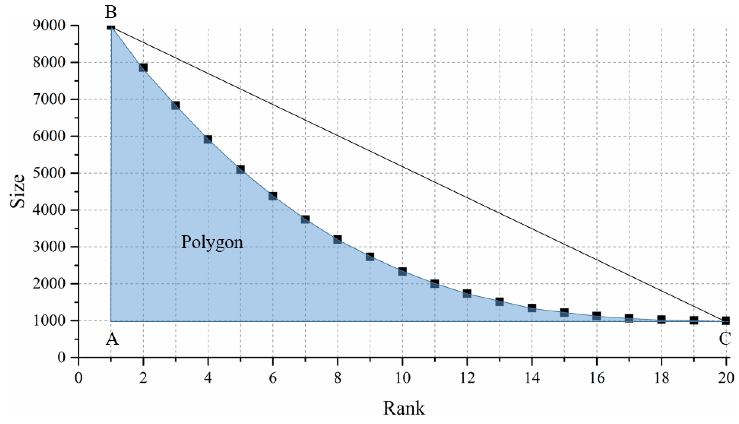
3.1. Ratio of Areas in Rank-Size Plots

A rank-size plot is a scatter plot to display the distribution of size by rank. For example, Figure 2 is the rank-size plot of a set of numbers. These numbers are ranked in descending order, and each number is represented by a point. With the rank-size plot, we define an index for further use; the index equals the ratio of Area 1 to Area 2 (referred to as RA hereafter), where Area 1 is the area of the polygon shown in Figure 2, and Area 2 is the area of the triangle ABC in the same figure.

Here is the mathematical expression of the defined RA. Let Y be a set of random numbers. Rank these numbers in increasing order, and then obtain $\mathrm{Y}=\left\{y_1,y_2,\dots ,y_n\right\}$, where $y_1\le y_2\le \dots \le y_n$. Let X be the orders of these increasing numbers, where $\mathrm{X}=\left\{x_1=1,x_2=2,\dots ,x_n=n\right\}$. The calculation method of RA is as follows:

$$\{\begin{array}{c}RA=Area1/Area2*100\%\\ Area1=-\frac{1}{2}\left[2x_n{y}_1-x_n{y}_n-x_1{y}_1+{\displaystyle {\displaystyle \sum }_{i=1}^{n-1}}\left(x_i{y}_{i+1}-x_{i+1}{y}_i\right)\right]\\ Area2=\frac{1}{2}\left(x_n-x_1\right)\left(y_n-y_1\right)\end{array}$$

(1)

(Note that a tool developed for calculating the RA is available in the supplementary material.)

3.2. Characterize the Traffic Condition of a Network

The traffic condition of a traffic network can be characterized from the perspective of spatial heterogeneity. By spatial heterogeneity we mean the traffic condition of roads varies largely in different spatial locations; some roads are likely to be congested at one moment, whereas the others are probably not at the same moment. For a specific moment, vehicle speeds of all roads in the traffic network can be regarded as a set of random numbers. This set of numbers can be employed to calculate the RA, which is a measurement of the heterogeneity of these numbers and is actually also the characterization of the traffic condition behind these numbers.

3.3. Characterize the Traffic Condition of a Single Road

The traffic condition of a single road in a traffic network can be characterized from the perspective of temporal heterogeneity. By temporal heterogeneity, we mean the traffic condition of a single road changes with time. This change can easily be understood: a road is likely to be more congested during the morning and evening rush hours, while is less congested at the other time. The changing vehicle speed of one road leads to a heterogeneity. The key point is the degree of heterogeneity reflects the traffic condition of one road during a specific period and this degree is comparable to another. In this study, the traffic condition of a single road is measured by the RA, where a set of vehicle speeds of the road is employed as input for the measurement.

4. Traffic Conditions Characterized

4.1. The Measuring Scale

The measuring scale is a significant concept in processing geographic information. Without an appropriate measuring scale, the length of the British seacoast is even meaningless [21,22,23]. For the pioneering work in characterizing the heterogeneity [13,14], the measuring scale is also very important. In the work conducted by Jiang and Yin [14], the Koch curve is measured using a set of selected scales including 1/3, 1/9, and 1/27, rather than using every scale ranging from 1/27 to 1/3. In the work conducted by Gao, et al. [13], the traffic condition of San Francisco Bay Area is measured using a rather coarse scale: Traffic conditions of roads are divided into four levels, and then the measuring method (i.e., the proposed CRG index) was performed based on these four levels. Though coarse, the measuring scale performed quite well in that work.

The characterization of heterogeneity relies on an appropriate measuring scale, but more studies are needed on the selection of an ideal measuring scale. The research on selection strategies lies outside the scope of this study. For this reason and considering that a coarse measuring scale may reduce errors in characterizing heterogeneity, this study follows the pioneering work in adopting a relatively coarse measuring scale in characterizing traffic conditions. In specific, the accuracy of vehicle speeds in the raw data is 0.1 km/h, meaning that the measuring scale is 0.1 km/h. This measuring scale is too fine, and a coarse one, 20 km/h, is adopted in this study. In other words, the vehicle speeds ranging from 0 to 20 km/h are simply regarded as 20 km/h, and the ones ranging from 20 km/h to 40 km/h are classified as 40 km/h, and so on (another method to use the measuring scale r is to classify values from r to 2*r as r. This method was not adopted in this study, but note that there exists no differences between this method and the method adopted in this study in terms of calculating the RA). Note that the adopted measuring scale here may not be the best one, and a comparison among different measuring scales is presented in Section Experiments.

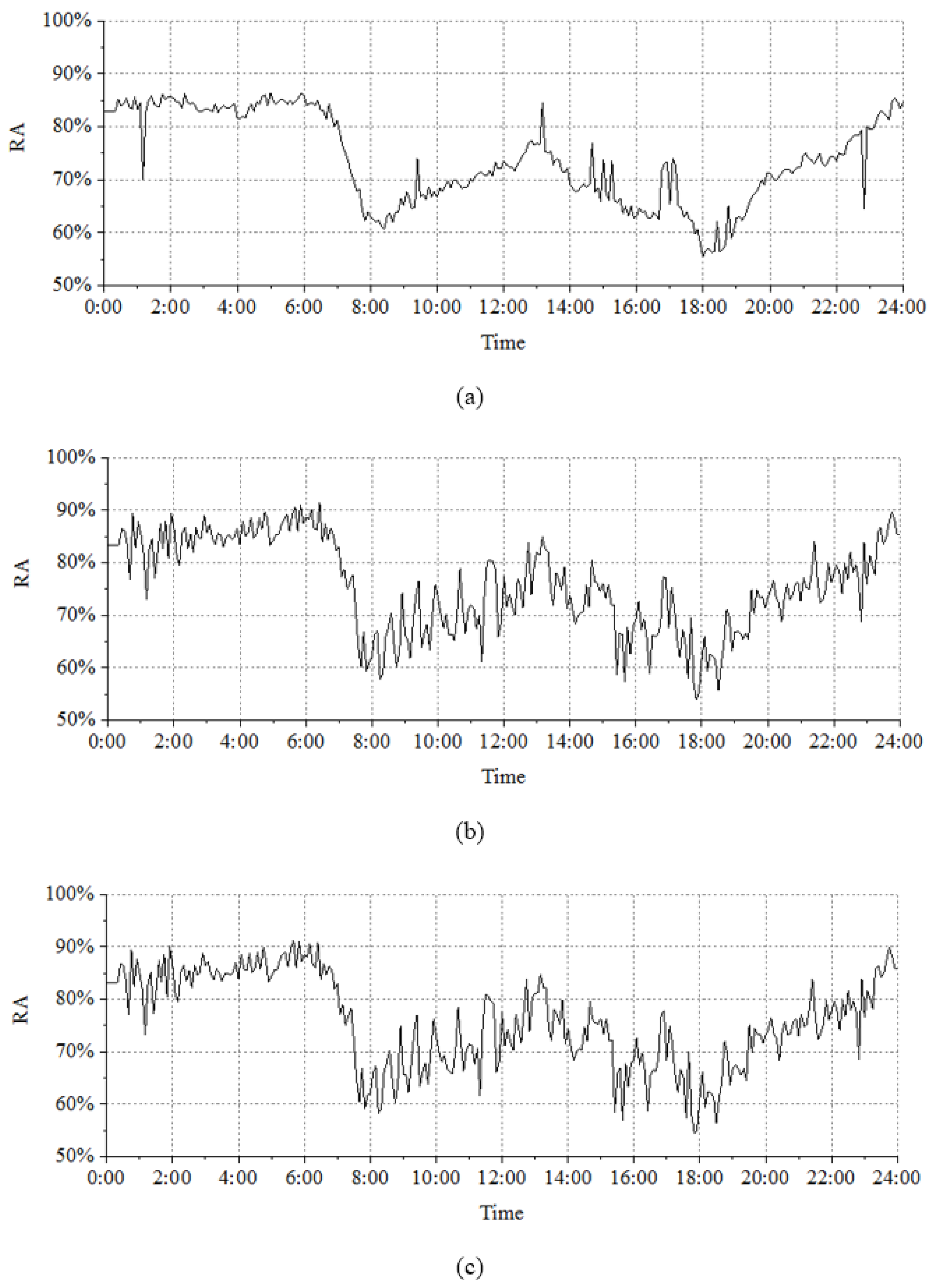
4.2. Traffic Conditions of Shenzhen in One Week

Traffic conditions of Shenzhen are characterized by the RA every five minutes from the perspective of spatial heterogeneity. The value of RA is accurate to four decimal places (i.e., 0.01%). This section illustrates the characterized traffic conditions on a Monday (19 October 2015), a Wednesday (21 October 2015), a Friday (23 October 2015), and a Sunday (25 October 2015), as shown in Figure 3. Not all the days in a week are illustrated here, because the traffic conditions on weekdays (or weekends) are similar.

The value of the RA reflects the traffic condition of the road network of Shenzhen; the smaller the RA is, the more congested the traffic network is. In other words, the value of the RA is inversely proportional to the degree of traffic congestion. According to this inverse relationship, some patterns can be easily seen from Figure 3: For weekdays, the morning rush period begins from about 6:30 and peaks around 8:30, and the evening rush period starts from 17:00 and peaks around 18:30; whereas for weekends, the morning rush period begins later than that of weekdays. These patterns are common in real life, suggesting that the characterized traffic conditions are meaningful.

4.3. Congestion-Prone Roads in Shenzhen

Traffic conditions can also be characterized from the perspective of temporal heterogeneity. From this perspective, vehicle speeds of a single road during a period form a heterogeneous group of numbers (referred to as the Group). The heterogeneity of this group can be measured by the RA. The larger the value of the RA is, the better the traffic condition over the period is. Traffic conditions from the perspective of temporal heterogeneity are comparable between two roads, so the corresponding RA can be employed to find out congestion-prone roads from a traffic network.

For the 358 monitored roads in Shenzhen, the first 10 congestion-prone roads are listed in

Table 1. First ten congestion-prone roads in Shenzhen.

Order	Name of Road	RA	Order	Name of Road	RA
1	Mei Long (S. to N.)	28.22%	6	Chang Chun (S. to N.)	51.22%
2	Hua Qiang (N. to S.)	42.16%	7	Ji Hua (N. to S.)	52.26%
3	Bai Shi (W. to E.)	47.74%	8	Xin An (W. to E.)	60.63%
4	Liu Xian San (S. to N.)	48.43%	9	Song Ming Da Dao (W. to E.)	61.32%
5	Luo Hu Tao Yuan (E. to W.)	50.17%	10	Luo Hu Tao Yuan (W. to E.)	65.85%

Note: E. = east; W. = west; S. = south; and N. = north.

. The corresponding values of RA are also included in this table. The road with a small RA is considered as a congestion-prone road in this study, because a small RA means that most members of the Group are low vehicle speeds.

5. Experiments

We have shown in the above section that traffic conditions can be characterized by using the proposed RA from the perspective of either spatial heterogeneous or temporal heterogeneous. This section presents experiments on characterizing the traffic condition with different methods.

5.1. Effect of the Measuring Scale

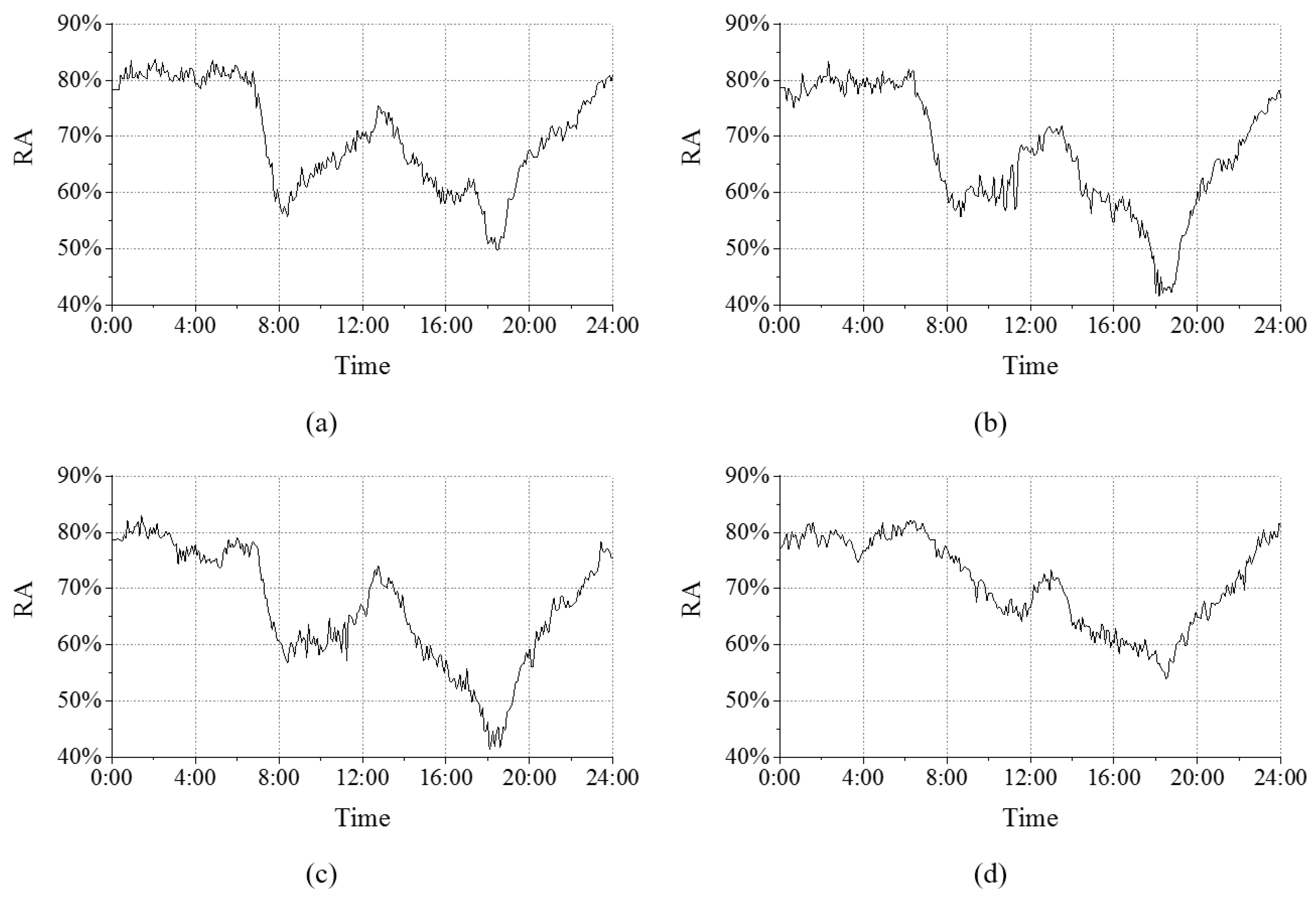
A measuring scale of 20 km/h was employed in the above section to characterize traffic conditions of Shenzhen. Though the characterization reflects key traffic patterns, the adopted measuring scale may not be the best choice since the scale is relatively coarse. To examine the effect of the measuring scale, a set of finer scales is adopted for the characterization in this section. This scale set includes 10 km/h, 1 km/h, and 0.1 km/h. Figure 4 shows the traffic conditions characterized with these measuring scales for the road network of Shenzhen on 19 October 2015 (Monday).

As can be seen from Figure 4, the rush hours in the morning and in the evening are characterized by all the three measuring scales, but outliers are included in comparison to Figure 3a (e.g., the values of the RA at 1:10 and 22:50). In addition, compared to Figure 3a, more noise is introduced in Figure 4 when characterizing with a finer measuring scale, making the RA curve fluctuate more and more especially when comparing among Figure 3a and Figure 4a,b (e.g., the RA values between 8:00 and 12:00). The outliers and noise demonstrate that (1) the measuring scale has an effect on the characterization of heterogeneity; (2) a coarse measuring scale seems to perform better than a fine measuring scale; and (3) for the characterization of traffic conditions, 20 km/h is a satisfying measuring scale. For other case studies (e.g., the characterization of the change of PM 2.5), more research on the adoption strategy of measuring scales is required.

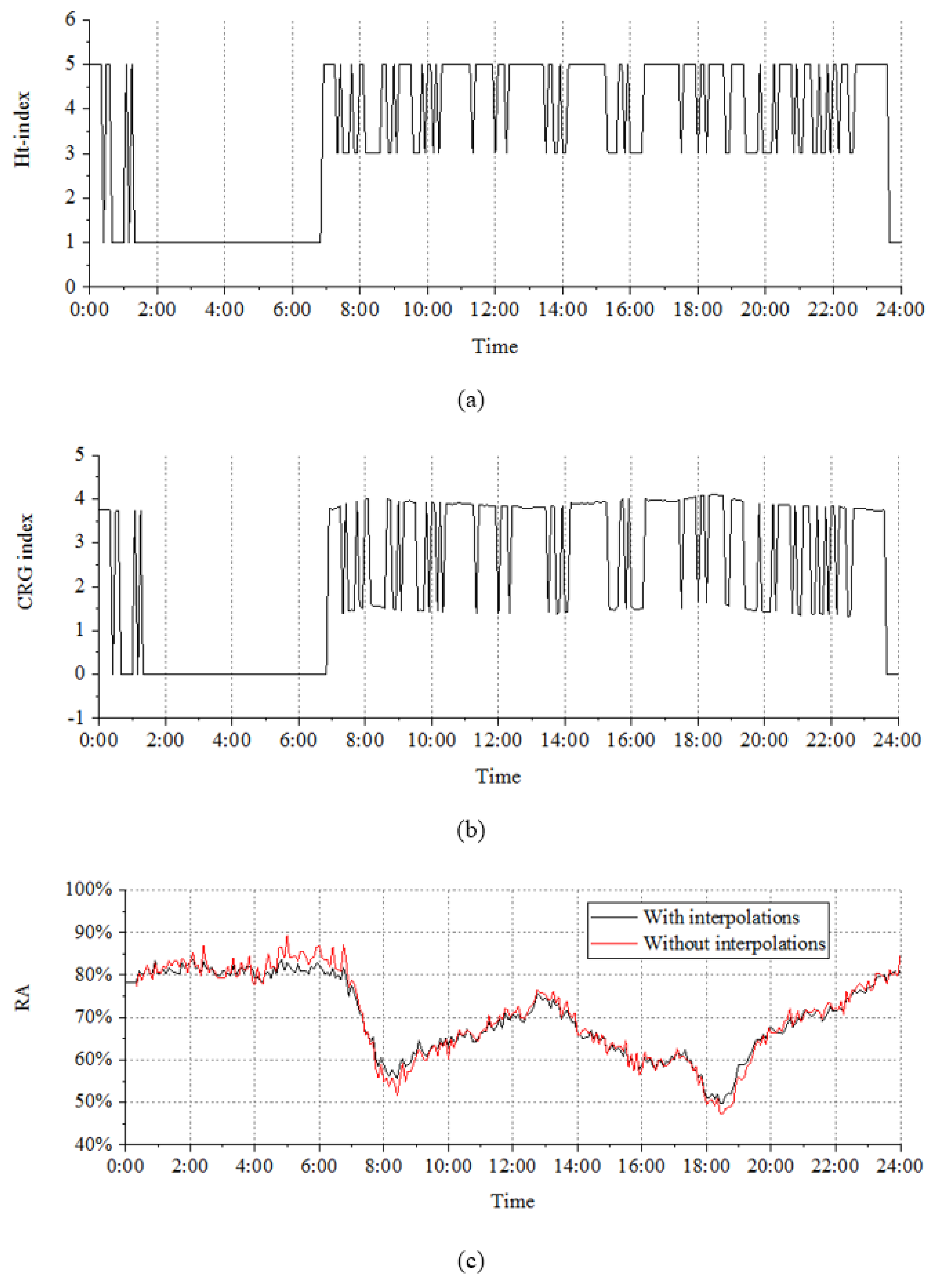
5.2. Comparison to Ht-Index/CRG Index

In the pioneering work conducted by Jiang and Yin [14] and the one by Gao, et al. [13], the ht-index and the CRG index were employed to characterize the heterogeneity behind geographic features (including road networks), respectively. This section compares the traffic conditions of Shenzhen on 19 October 2015 (Monday) characterized in this work (Figure 3a, by the proposed RA) and the ones characterized by using the ht-index (Figure 5a)/CRG index (Figure 5b).

As can be seen from Figure 5a,b, (1) both the ht-index and the CRG index changes along the time, with a range of 1–5 and 0–4, respectively; (2) the CRG index seems to be more sensible than the ht-index to the change of traffic condition, as the former index sometimes fluctuates while the latter one remains unchanged (e.g., the period from 14:00 to 15:20). However, neither the ht-index nor the CRG index is able to capture the pattern of traffic conditions (such as the morning/evening rush hour). In other words, compared to the proposed method in this work, the ht-index and the CRG index are less effective in characterizing traffic conditions.

5.3. Necessity of Interpolations

The interpolation is a significant step in processing the raw traffic data before the characterization of traffic conditions. In this work, interpolations were performed based on the hypothesis that the traffic condition of a road is changing gradually. This section is not aimed to test this hypothesis, but aimed at demonstrating the necessity of interpolations. For this purpose, traffic conditions of Shenzhen in a one-day period (i.e., 19 October 2015) are characterized based on raw data with and without interpolations, respectively, as shown in Figure 5c.

As can be seen from Figure 5c, the fluctuation of the RA curve without interpolations is greater than the one with interpolations, demonstrating that interpolations are necessary. Moreover, it should be noted that the first several values are missing on the RA curve without interpolations. This is because of the missing raw data during that period, which may be caused by errors in the traffic monitoring system. Though the raw data are not complete, the RA curve with interpolations is not interrupted, providing a continuous view of the change of the traffic condition.

6. Discussion

We have shown that the proposed method can effectively characterize traffic conditions from the perspective of spatial-temporal heterogeneity. In this section, we discuss three issues, i.e., (1) the mathematical meaning of the proposed method and why it can be utilized for the characterization; (2) the boundary (i.e., the lower limit and the upper limit) of the proposed RA; and (3) why the proposed RA performs better than the ht-index and the CRG index.

From the mathematical perspective, the traffic condition characterized by using the proposed method is in fact the pattern of a set of values exhibiting a heavy-tailed distribution, or the pattern of the rank-size plot for a dataset. Traffic data such as vehicle speeds usually follow a heavy-tailed distribution; for example, there are far more roads with low vehicle speeds than ones with high vehicle speeds (referred to as Condition 1), or vice versa (referred to as Condition 2). Changes of traffic conditions are in fact transformations between Condition 1 and Condition 2, so the proposed method can effectively characterize traffic conditions.

The proposed RA, as an index, is in fact a measurement that forms a relationship between mathematics and empirical research [24,25]. A good index should have a clear boundary, which includes a lower limit and an upper limit. For the proposed RA, its lower limit is 0 (approaches but never actually hits zero), which means the dataset to be characterized is very heavy-tailed. The upper limit of the RA is 2 (approaches but never actually hits two), which means the dataset to be characterized is very light-tailed (i.e., non-heavy-tailed). In particular, the RA value of 1 is actually the boundary of a heavy-tailed distribution and a non-heavy-tailed distribution.

Both the ht-index and the CRG index in the pioneering work can be employed to characterize a heavy-tailed dataset (the CRG index also applies to a non-heavy-tailed dataset), but are less effective than the proposed RA in this work. The reason is that the characterization based on either the ht-index or the CRG index relies on the number of levels in the hierarchy formed by the head/tail breaks method [26,27], but this number is likely to remain unchanged as the change of the dataset to be characterized. Instead, the proposed RA relies on the pattern of the dataset displayed in a rank-size plot; this pattern changes significantly along with the dataset.

7. Conclusions

The traffic condition has become a major concern for a large number of cities all over the world, and it still seems to be increasingly serious as there are more and more traffic congestions. To manage and control traffic congestions, one significant step is to characterize traffic conditions accurately and in a timely way, which is actually not an easy task. In the field of transportation, traffic conditions are usually characterized from the perspective of travel time or the average vehicle speed.

In this work, traffic conditions were characterized from a novel perspective, i.e., the perspective of spatial-temporal heterogeneity. In particular, the traffic data utilized were vehicle speeds of roads in a traffic network. These vehicle speeds were considered to be statistically non-stationary (i.e., heterogeneous) in time and space. The traffic condition of a road network was characterized from the perspective of spatial heterogeneity, whereas the traffic condition of a single road was characterized from the perspective of temporal heterogeneity. To measure the heterogeneity, a new measurement, which has been termed as the RA, was proposed and included in the characterization method. The performance of this proposed method was tested with real-life traffic data, and the results demonstrated its effectiveness. Moreover, the proposed RA was compared to similar measuring methods such as the ht-index and the CRG index, and the RA performed the best of the three methods. In the future, we plan to test the proposed method with traffic data of more cities.