
Land Surface Water Mapping Using Multi-Scale Level Sets and a Visual Saliency Model from SAR Images

Abstract
:1. Introduction
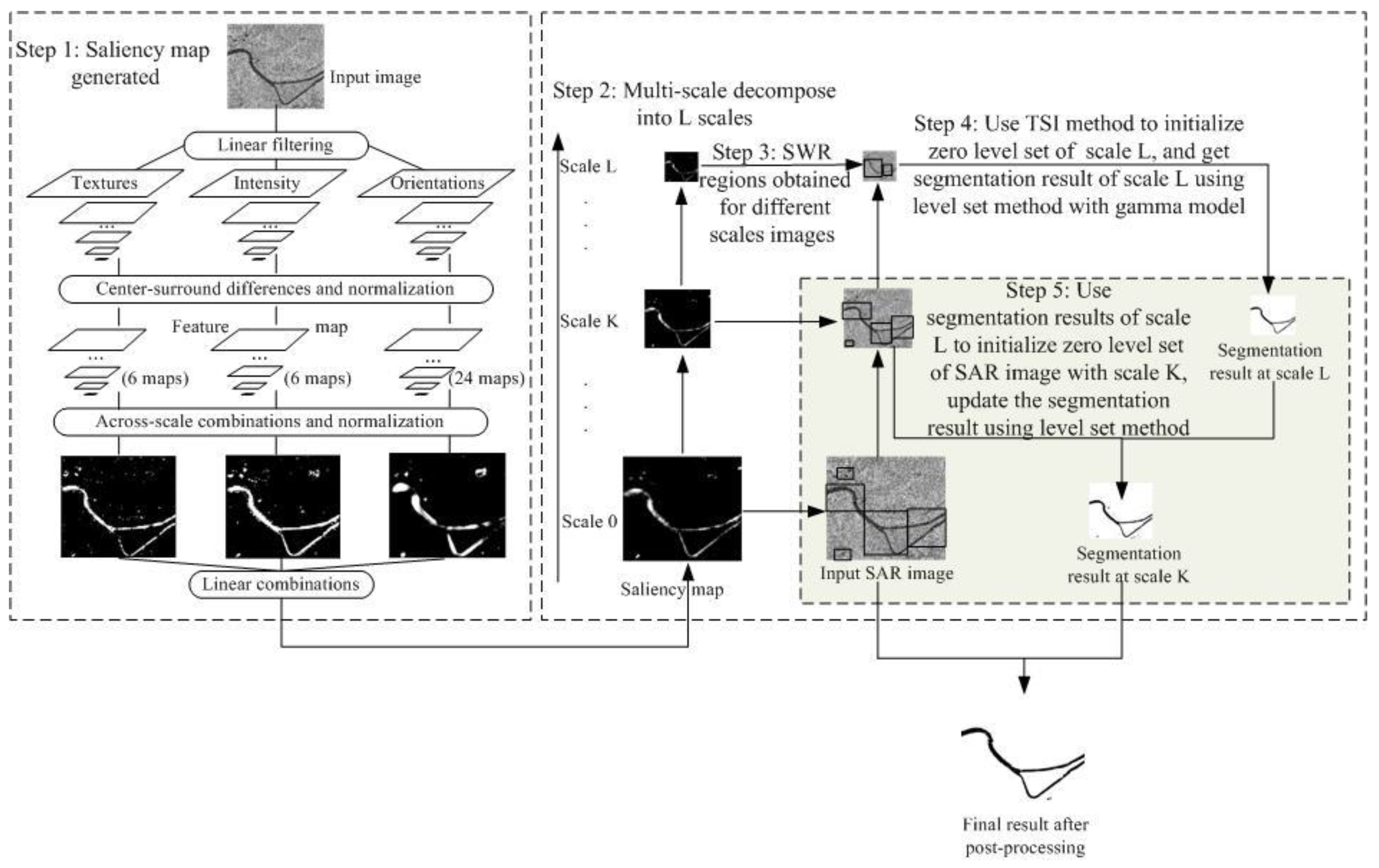
2. Proposed Method
2.1. Improved TW-Itti Model
2.2. Adaptive Multi-Scale Level Set Method Based on the Gamma Model
- (1)
- Initialize the level set function using Equation (15);
- (2)
- Evolve the level set function according to Equations (13) and (14);
- (3)
- Check whether the evolution is stationary. If not, return to Step 2.
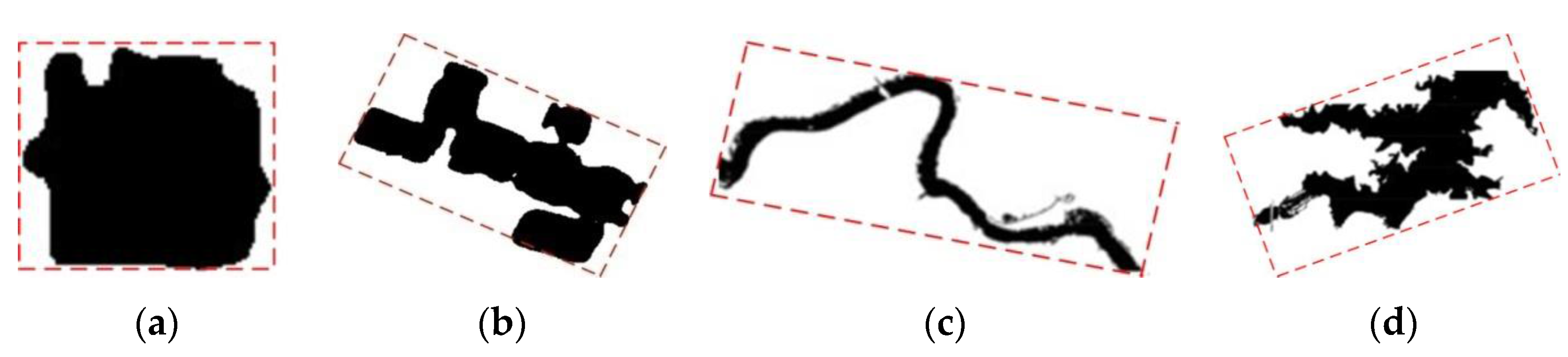
2.3. Post-Processing: Using Object-Oriented Geometrical Feature
3. Experimental Data Set
- (1)
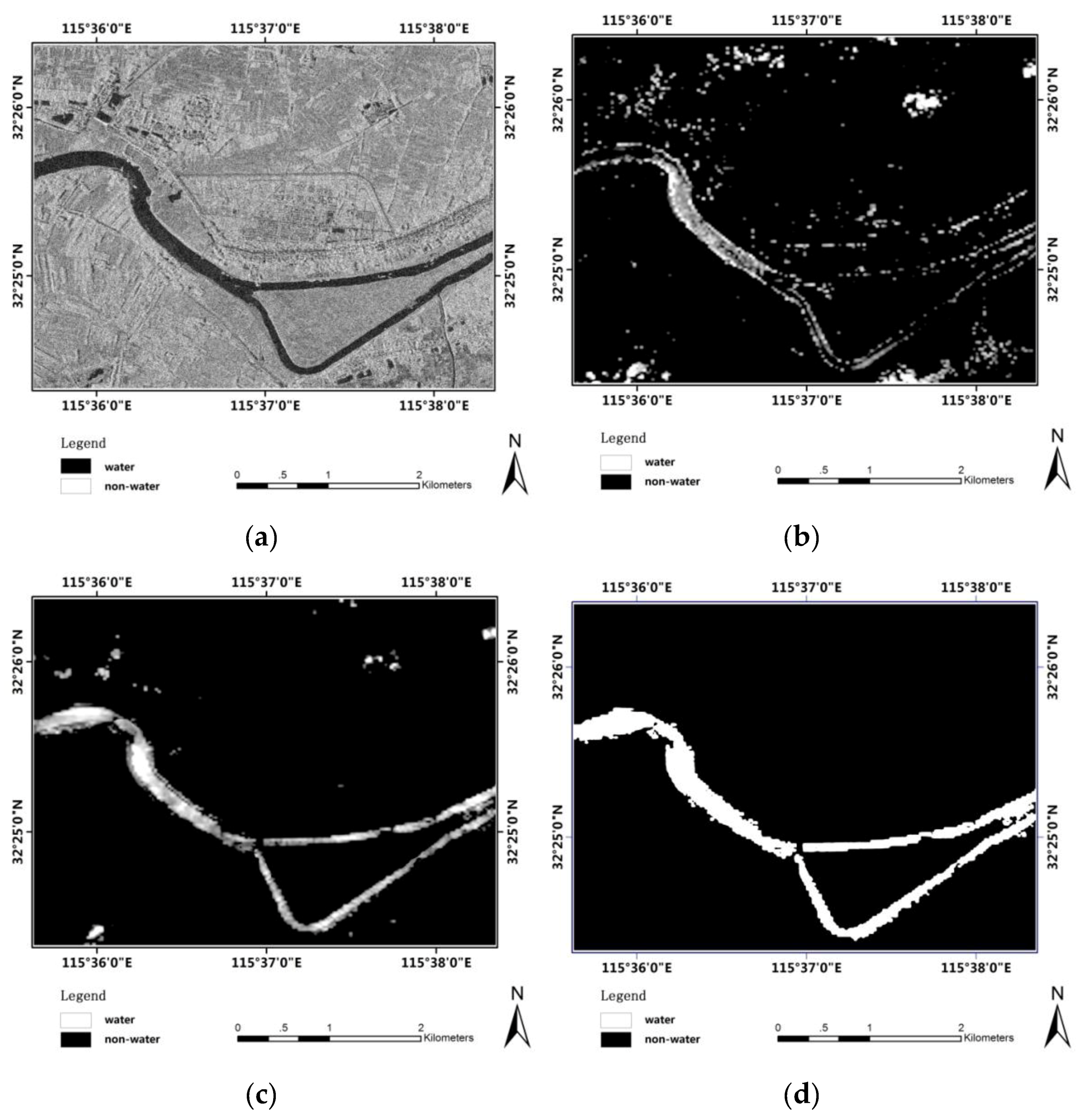
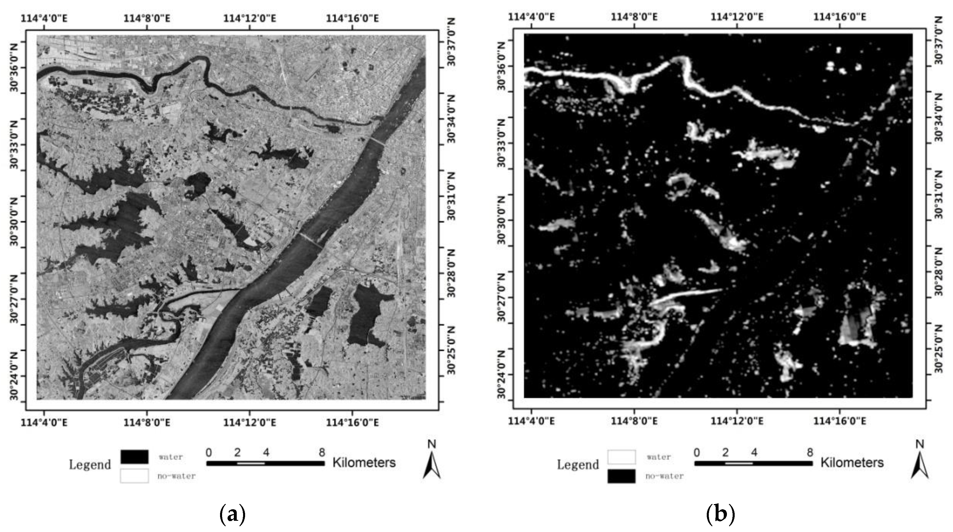
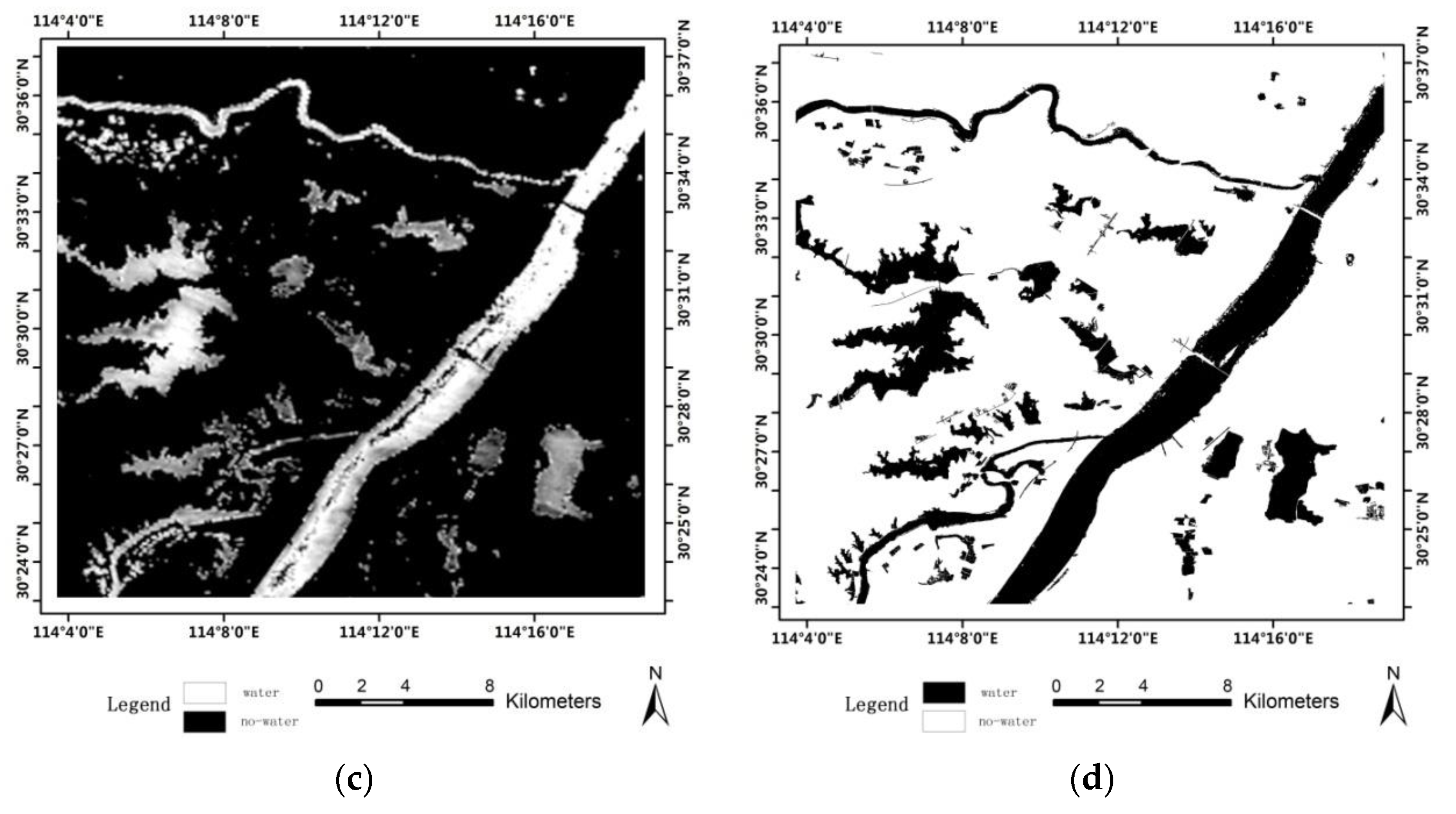
- Study Area of Huai River: Huai River catchment around eastern China is taken as one of the study areas. The Radarsat 2 images (VV polarization) at a spatial resolution of 3 m were acquired on 7 December 2009. A Google map image of 0.5m resolution with the same region and same season is used as the true water class image, then manual water extraction in this google image is used for reference to check the accuracy of the water extraction process.
- (2)
- Study Area of Hanjiang and Changjiang River: Hanjiang River is the largest branch of Changjiang River, and they are located in Wuhan City, Hubei Province, China. The TerraSAR-X images (VV polarization) at a spatial resolution of 1 m were acquired on 9 October 2008. A vector map of the same region supported by Map Institute of Hubei Province is used for reference to check the accuracy of the water extraction process.
4. Results and Discussion
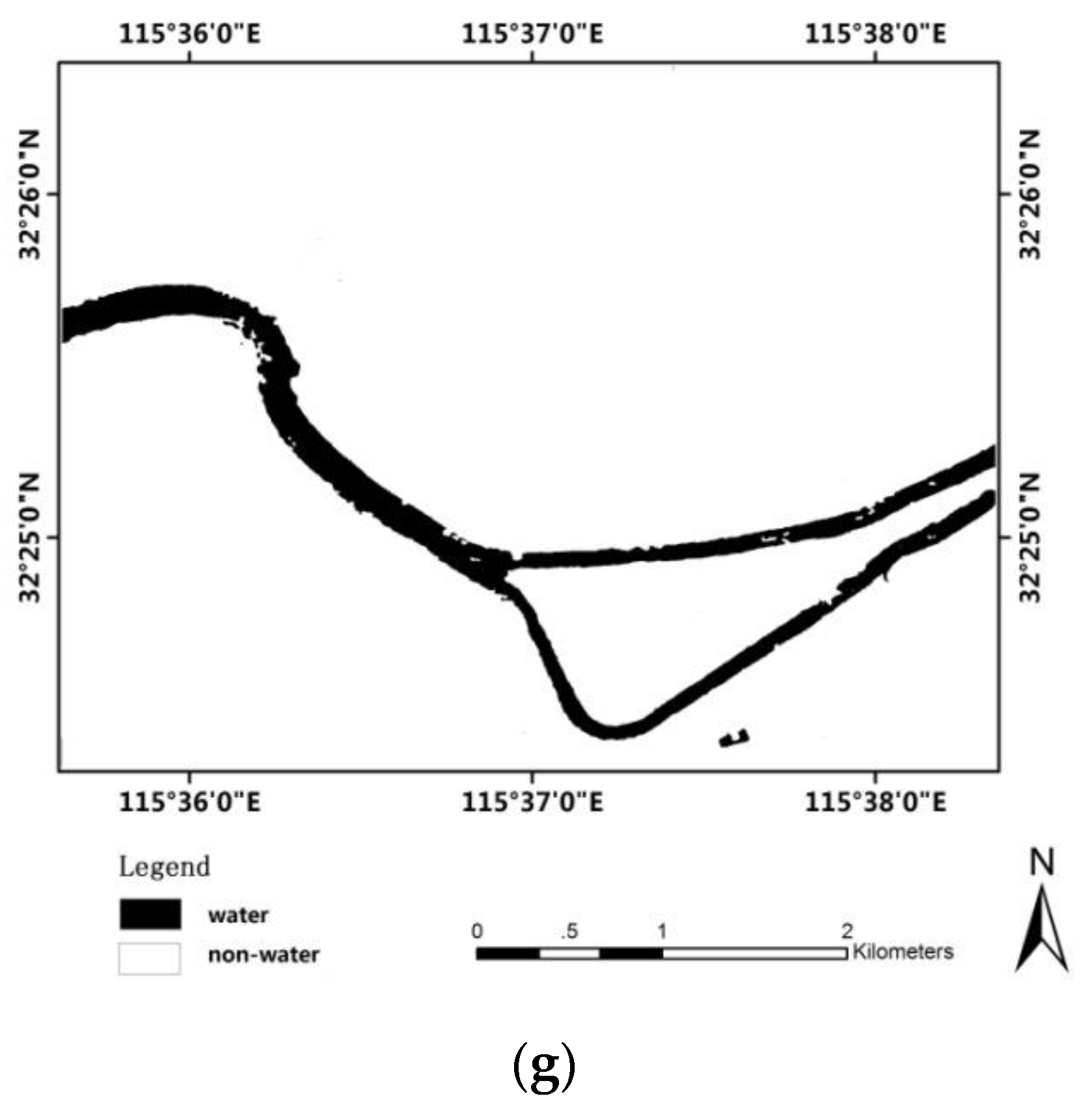
4.1. Experiment on Radarsat-2 Image
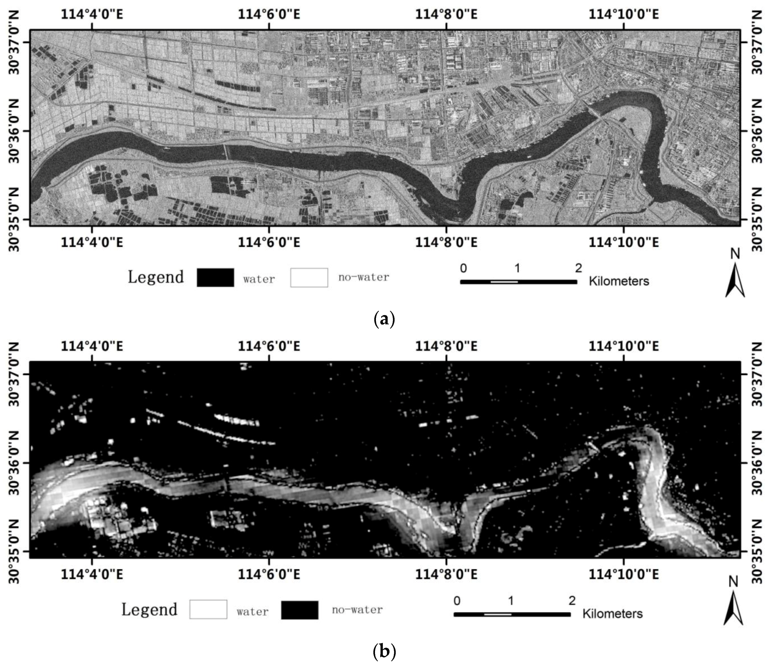
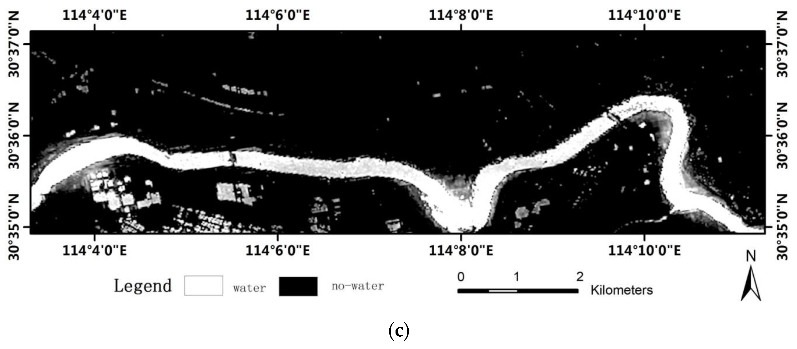
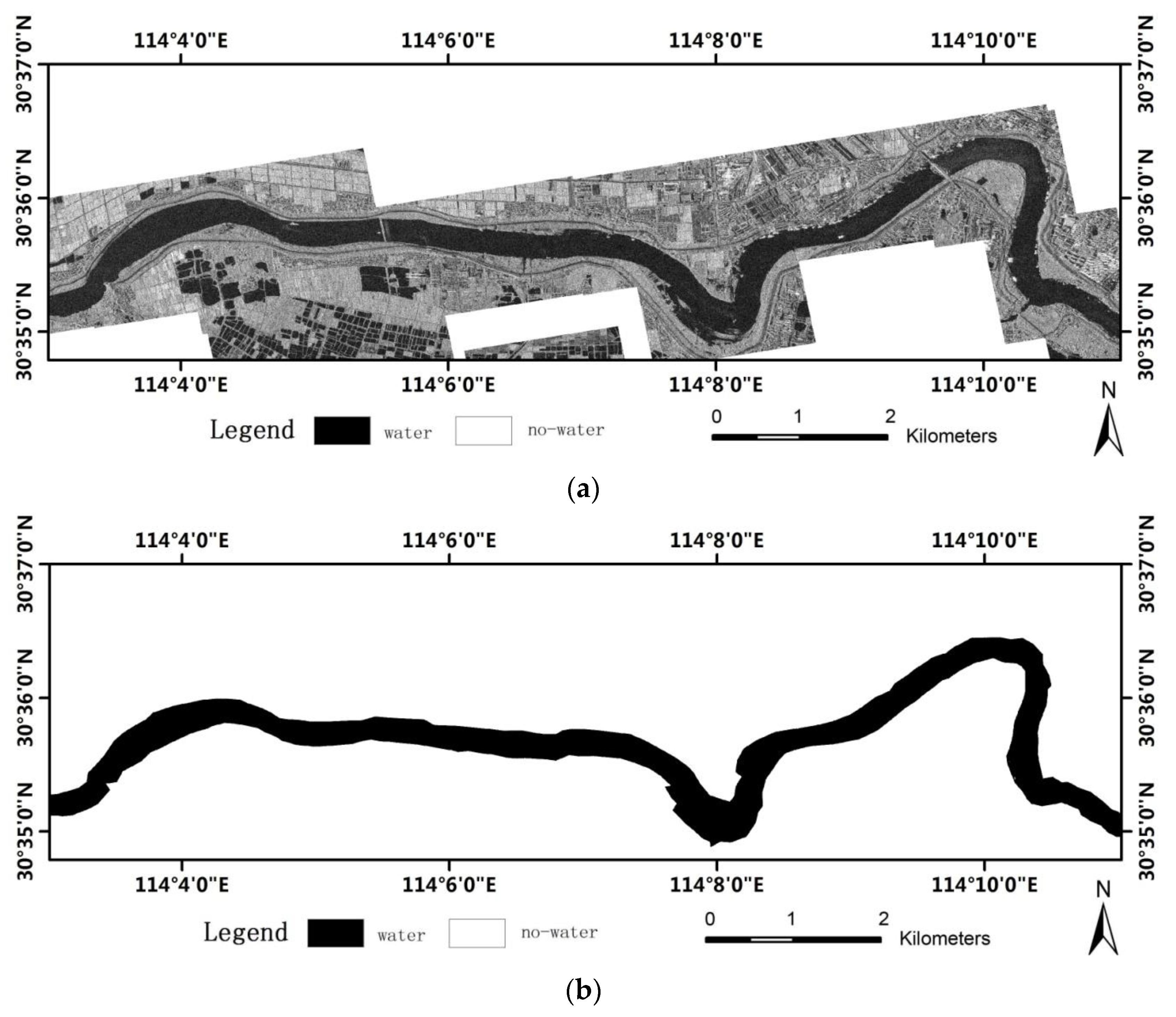
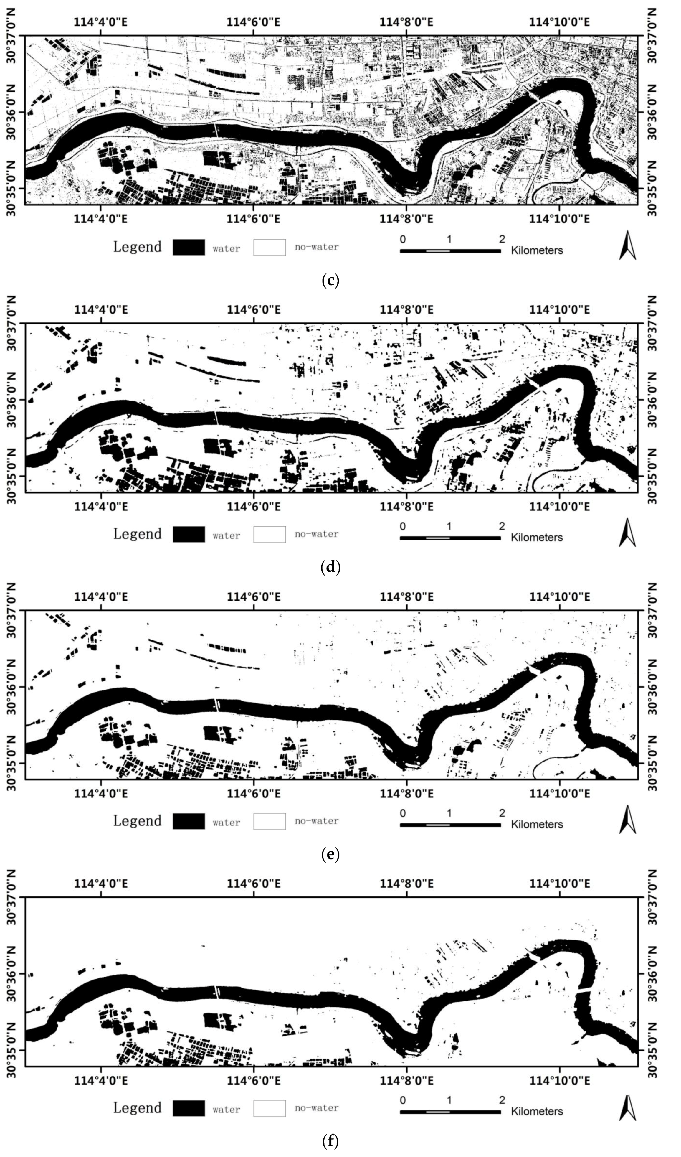
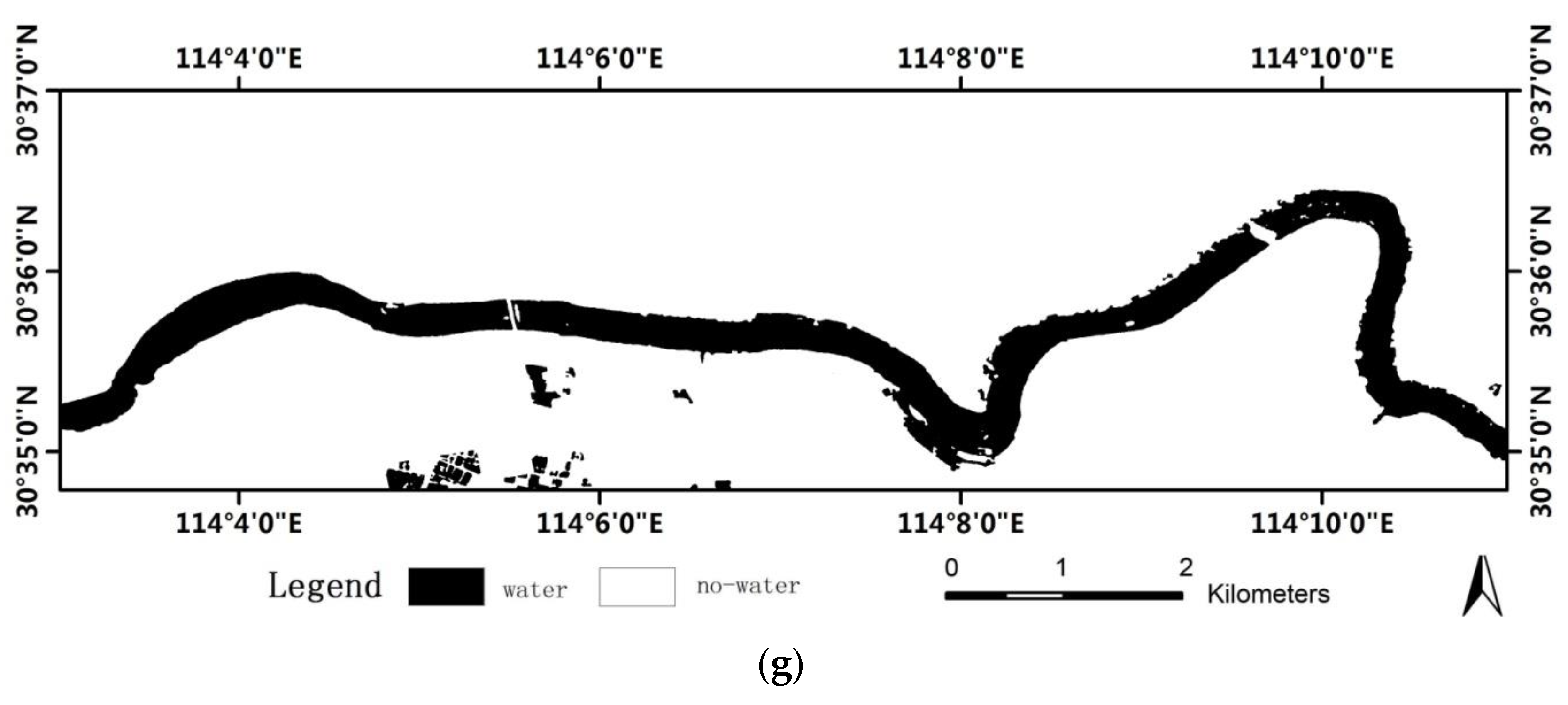
4.2. Experiment on TerraSAR-X Imagery
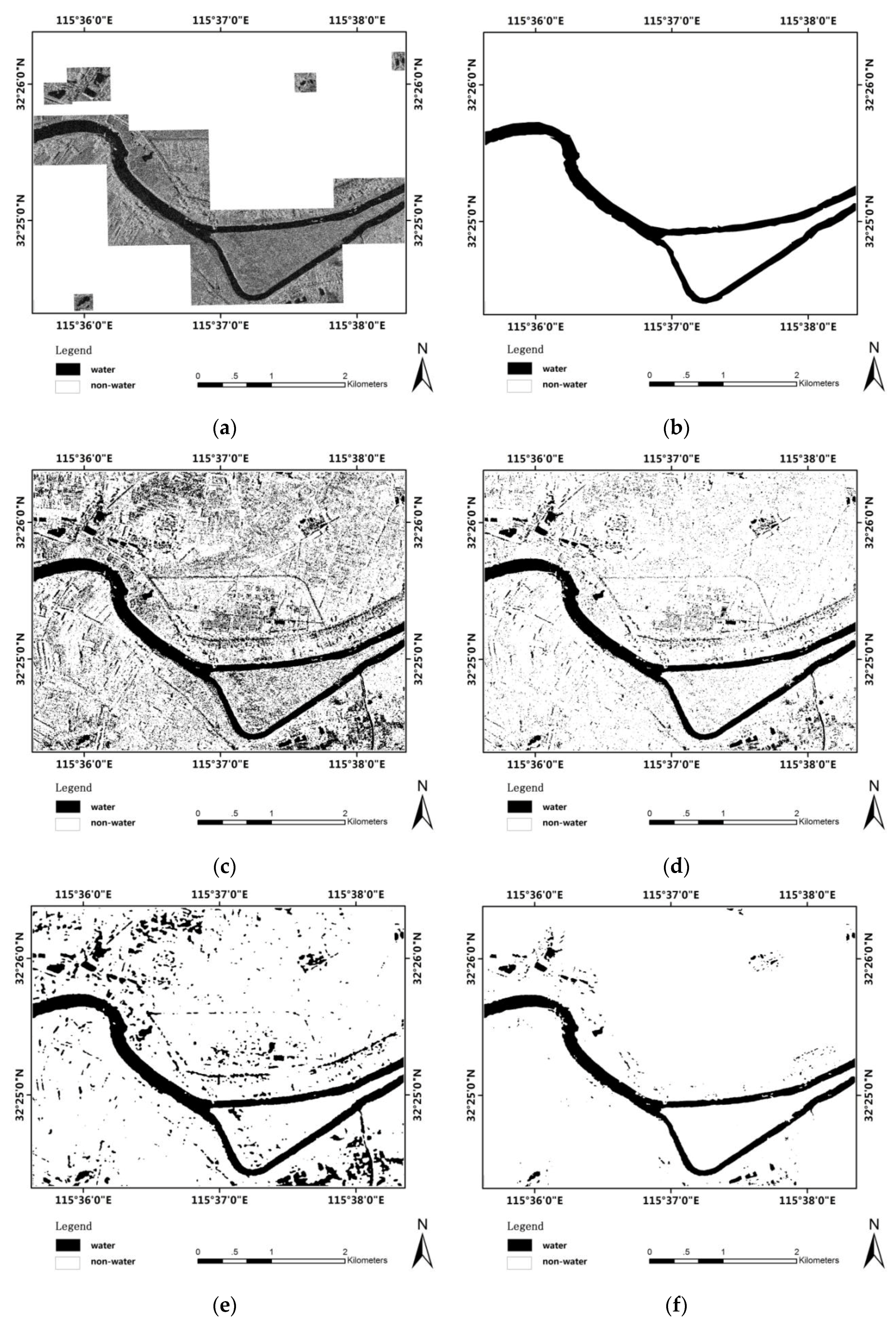
4.3. Applications to Large-Area SAR Images
4.4. Accuracy Analysis and Discussion
- (1)
- (2)
- Compared with the state-of-the-art methods (ALG1, ALG2 and ALG3), the method of integration using the multi-scale technique and visual saliency model produced better accuracy.
- (3)
5. Conclusions
Acknowledgments
Author Contributions
Conflicts of Interest
Abbreviations
| SAR | Synthetic Aperture Radar |
| MLSVS | multi-scale level sets and visual saliency |
| SWR | suspected water regions |
| GLCM | Gray Level Co-occurrence Matrix |
| LSW | Land Surface Water |
References
- Thomas, H.; Sandro, M.; Andre, T.; Achim, R.; Manfred, B. Extraction of water and flood areas from SAR data. In Proceedings of the 7th European Conference on Synthetic Aperture Radar (EUSAR), Friedrichshafen, Germany, 2–5 June 2008; pp. 1–4.
- Lee, J.S.; Iurkevich, I. Segmentation of SAR Image. IEEE Trans. Geosci. Remote Sens. 1989, 27, 981–990. [Google Scholar] [CrossRef]
- Sahoo, P.K.; Soltani, S.; Wong, A.K.C. A survey of thresholding techniques. Comput. Vis. Graph. Image Process. 1988, 41, 233–260. [Google Scholar] [CrossRef]
- Fiortoft, R.; Lopes, A.; Marthon, P. An optimal multi edge detector for SAR image segmentation. IEEE Trans. Geosci. Remote Sens. 1998, 36, 793–802. [Google Scholar] [CrossRef]
- Oliver, C.; Connell, I.M.; White, R.G. Optimum edge detection in SAR. SPIE Satell. Remote Sens. 1995, 2584, 152–163. [Google Scholar] [CrossRef]
- Cook, R.; Connell, I.M.; Oliver, C.J. MUM Segmentation for SAR Images. Proc. SPIE 1994, 2316, 92–103. [Google Scholar]
- Udupa, J.K.; Samarasekera, S. Fuzzy connectedness and object definition: Theory, algorithms, and applications in image segmentation. Graph. Models Image Process. 1996, 58, 246–261. [Google Scholar] [CrossRef]
- Deng, H.; Clausi, D. Unsupervised segmentation of synthetic aperture radar sea ice imagery using a novel Markov random field model. IEEE Trans. Geosci. Remote Sens. 2005, 43, 528–538. [Google Scholar] [CrossRef]
- Stéphane, D.; Grégoire, M. Unsupervised multiscale oil slick segmentation from SAR images using a vector HMC model. Pattern Recognit. 2007, 40, 1135–1147. [Google Scholar]
- Gan, L.; Wu, Y.; Wang, F.; Zhang, P.; Zhang, Q. Unsupervised SAR image segmentation based on triplet Markov fields with graph cuts. IEEE Geosci. Remote Sens. Lett. 2014, 11, 853–857. [Google Scholar] [CrossRef]
- Wang, F.; Wu, Y.; Zhang, Q.; Zhao, W.; Li, M.; Liao, G.S. Unsupervised SAR image segmentation using higher order neighborhood-based triplet Markov fields model. IEEE Trans. Geosci. Remote Sens. 2014, 52, 5193–5205. [Google Scholar] [CrossRef]
- Wang, Y.; Li, Y.; Zhao, Q.H. Segmentation of high-resolution SAR image with unknown number of classes based on regular tessellation and RJMCMC algorithm. Int. J. Remote Sens. 2015, 36, 1290–1306. [Google Scholar] [CrossRef]
- Huang, B.; Li, H.; Huang, X. A level set method for oil slick segmentation in SAR images. Int. J. Remote Sens. 2005, 26, 1145–1156. [Google Scholar] [CrossRef]
- Silveira, M.; Heleno, S. Separation between water and land in SAR images using region-based level sets. IEEE Geosci. Remote Sens. Lett. 2009, 6, 471–475. [Google Scholar] [CrossRef]
- Zou, P.F.; Li, Z.; Tian, B.S.; Guo, L.J. A level set method for segmentation of high-resolution polarimetric SAR images using a heterogeneous clutter model. Remote Sens. Lett. 2015, 6, 548–557. [Google Scholar] [CrossRef]
- Yin, J.J.; Yang, J. A modified level set approach for segmentation of multiband polarimetric SAR images. IEEE Trans. Geosci. Remote Sens. 2015, 52, 7222–7232. [Google Scholar]
- Chan, T.; Vese, L. Active contours without edges. IEEE Trans. Image Process. 2001, 10, 266–277. [Google Scholar] [CrossRef] [PubMed]
- Itti, L. Modeling primate visual attention. In Computational Neuroscience: A Comprehensive Approach; Feng, J., Ed.; CRC Press: Boca Raton, FL, USA, 2003; pp. 635–655. [Google Scholar]
- Itti, L.; Koch, C.; Niebur, E. Model of saliency-based visual attention for rapid scene analysis. IEEE Trans. Pattern Anal. Mach. Intell. 1998, 20, 1254–1259. [Google Scholar] [CrossRef]
- Itti, L.; Gold, C.; Koch, C. Visual attention and target detection in cluttered natural scenes. Opt. Eng. 2001, 40, 1784–1793. [Google Scholar]
- Walther, D.; Rutishauser, U.; Koch, C. Selective visual attention enables learning and recognition of multiple objects in cluttered scenes. Comput. Vis. Image Underst. 2005, 100, 41–63. [Google Scholar] [CrossRef]
- Li, Z.Q.; Fang, T.; Huo, H. A saliency model based on wavelet transform and visual attention. SCIENCE CHINA Inf. Sci. 2010, 53, 738–751. [Google Scholar] [CrossRef]
- Gao, L.N.; Bi, F.K.; Yang, J. Visual attention based model for target detection in large-field images. J. Syst. Eng. Electron. 2011, 22, 150–156. [Google Scholar] [CrossRef]
- Li, Z.C.; Itti, L. Saliency and gist features for target detection in satellite images. IEEE Trans. Image Process. 2011, 20, 2017–2029. [Google Scholar] [PubMed]
- Sui, H.G.; Xu, C.; Liu, J.Y.; Sun, K.M.; Wen, C.F. A novel multi-scale level set method for SAR image segmentation based on a statistical model. Int. J. Remote Sens. 2012, 33, 5600–5614. [Google Scholar] [CrossRef]
- Otsu, N. A threshold selection method from gray-level histogram. IEEE Trans. Syst. Man Cybern. 1979, 9, 62–66. [Google Scholar]
- Haralick, R.M.; Shanmugam, K.; Dinstein, I. Textural features for image classification. IEEE Trans. Syst. Man Cybern. 1973, 3, 610–621. [Google Scholar] [CrossRef]
- He, L.F.; Chao, Y.Y.; Suzuki, K.J. A run-based two-scan labeling algorithm. IEEE Trans. Image Process. 2008, 17, 749–756. [Google Scholar] [PubMed]
- User Guide of eCognition in Chinese. Available online: http://vdisk.weibo.com/s/zt_sYprKIffXK (accessed on 12 October 2015).
- Picco, M.; Palacio, G. Unsupervised classification of SAR images using markov random fields and Model. IEEE Geosci. Remote Sens. Lett. 2011, 8, 350–353. [Google Scholar] [CrossRef]
- Martinis, S.; Twele, A.; Voigt, S. Unsupervised extraction of flood-induced backscatter changes in SAR data using Markov image modeling on irregular graphs. IEEE Trans. Geosci. Remote Sens. 2011, 49, 251–263. [Google Scholar] [CrossRef]


| Name of water bodies | Huai River | Hanjiang River | Changjiang River |
|---|---|---|---|
| Sensor | Radarsat 2 (VV polarization) | TerraSAR-X (VV polarization) | TerraSAR-X (VV polarization) |
| Orbit | descending | ascending | ascending |
| Mode | Ulra-Fine | Spotlight | Spotlight |
| Date | 7 December 2009 | 9 October 2008 | 9 October 2008 |
| Resolution | 3 m | 1 m | 1 m |
| Image Size (pixels) | 3024 × 2263 | 7153 × 1948 | 15540 × 14550 |
| Method | Overall Accuracy (%) | Kappa Coefficient |
|---|---|---|
| Experiment on Radarsat-2 imagery | ||
| ALG1 | 79.22 | 0.262 |
| ALG2 | 92.39 | 0.530 |
| ALG3 | 91.38 | 0.511 |
| Proposed Method | 98.48 | 0.856 |
| Experiment on TerraSAR-X imagery | ||
| ALG1 | 81.80 | 0.434 |
| ALG2 | 88.71 | 0.577 |
| ALG3 | 94.17 | 0.731 |
| Proposed Method | 98.42 | 0.913 |
| Class | Reference Data | ||
|---|---|---|---|
| Water | Non-Water | Total | |
| Water | 351523 | 1383003 | 1734526 |
| Non-water | 38789 | 5069997 | 5108786 |
| Total | 390312 | 6453000 | 6843312 |
| Overall accuracy = 79.22% Kappa coefficient = 0.262 | |||
| Producer accuracy Water=351523/390312=90.06% Non-water=5069997/6453000=78.57% | User accuracy Water=351523/1734526=20.27% Non-water=5069997/5108786=99.24% | ||
| Class | Reference Data | ||
|---|---|---|---|
| Water | Non-Water | Total | |
| Water | 340153 | 470767 | 810920 |
| Non-water | 50159 | 5982233 | 6032392 |
| Total | 390312 | 6453000 | 6843312 |
| Overall accuracy = 92.39% Kappa coefficient = 0.53 | |||
| Producer accuracy
Water=340153/390312=87.15% Non-water=5982233/6453000=92.7% | User accuracy
Water=340153/810920=41.95% Non-water=5982233/6032392=99.17% | ||
| Class | Reference Data | ||
|---|---|---|---|
| Water | Non-Water | Total | |
| Water | 361014 | 560267 | 921281 |
| Non-water | 29298 | 5892733 | 5922031 |
| Total | 390312 | 6453000 | 6843312 |
| Overall accuracy = 91.38% Kappa coefficient = 0.511 | |||
| Producer accuracy Water=361014/390312=92.49% Non-water=5892733/6453000=91.32% | User accuracy Water=361014/921281=39.19% Non-water=5892733/5922031=99.51% | ||
| Class | Reference Data | ||
|---|---|---|---|
| Water | Non-Water | Total | |
| Water | 329671 | 43053 | 390312 |
| Non-water | 60641 | 6409947 | 6453000 |
| Total | 390312 | 6453000 | 6843312 |
| Overall accuracy = 98.48% Kappa coefficient = 0.856 | |||
| Producer accuracy
Water=329671/390312=84.46% Non-water=5069997/6453000=99.33% | User accuracy
Water=329671/390312=88.45% Non-water=6409947/6453000=99.06% | ||
© 2016 by the authors; licensee MDPI, Basel, Switzerland. This article is an open access article distributed under the terms and conditions of the Creative Commons Attribution (CC-BY) license (http://creativecommons.org/licenses/by/4.0/).
Share and Cite
Xu, C.; Sui, H.; Xu, F. Land Surface Water Mapping Using Multi-Scale Level Sets and a Visual Saliency Model from SAR Images. ISPRS Int. J. Geo-Inf. 2016, 5, 58. https://0-doi-org.brum.beds.ac.uk/10.3390/ijgi5050058
Xu C, Sui H, Xu F. Land Surface Water Mapping Using Multi-Scale Level Sets and a Visual Saliency Model from SAR Images. ISPRS International Journal of Geo-Information. 2016; 5(5):58. https://0-doi-org.brum.beds.ac.uk/10.3390/ijgi5050058
Chicago/Turabian StyleXu, Chuan, Haigang Sui, and Feng Xu. 2016. "Land Surface Water Mapping Using Multi-Scale Level Sets and a Visual Saliency Model from SAR Images" ISPRS International Journal of Geo-Information 5, no. 5: 58. https://0-doi-org.brum.beds.ac.uk/10.3390/ijgi5050058