Article

Automatic and Accurate Conflation of Different Road-Network Vector Data towards Multi-Modal Navigation

1
School of Human Settlements and Civil Engineering, Xi’An Jiaotong University, Xi’an 710049, China
2
Institute of Photogrammetry and Cartography, Technische Universität München, 80333 Munich, Germany
*
Authors to whom correspondence should be addressed.
ISPRS Int. J. Geo-Inf. 2016, 5(5), 68; https://0-doi-org.brum.beds.ac.uk/10.3390/ijgi5050068
Submission received: 3 February 2016 / Revised: 29 April 2016 / Accepted: 9 May 2016 / Published: 16 May 2016

Abstract

:
With the rapid improvement of geospatial data acquisition and processing techniques, a variety of geospatial databases from public or private organizations have become available. Quite often, one dataset may be superior to other datasets in one, but not all aspects. In Germany, for instance, there were three major road network vector data, viz. Tele Atlas (which is now “TOMTOM”), NAVTEQ (which is now “here”), and ATKIS. However, none of them was qualified for the purpose of multi-modal navigation (e.g., driving + walking): Tele Atlas and NAVTEQ consist of comprehensive routing-relevant information, but many pedestrian ways are missing; ATKIS covers more pedestrian areas but the road objects are not fully attributed. To satisfy the requirements of multi-modal navigation, an automatic approach has been proposed to conflate different road networks together, which involves five routines: (a) road-network matching between datasets; (b) identification of the pedestrian ways; (c) geometric transformation to eliminate geometric inconsistency; (d) topologic remodeling of the conflated road network; and (e) error checking and correction. The proposed approach demonstrates high performance in a number of large test areas and therefore has been successfully utilized for the real-world data production in the whole region of Germany. As a result, the conflated road network allows the multi-modal navigation of “driving + walking”.

1. Introduction

The word “conflation”, from the Latin con flare meaning “blow together”, is a legitimate word traditionally used to describe the merging of two manuscripts into a third combined version. Data conflation, in GIS environment, refers to a combining of two geospatial datasets to produce a third one which is “better” than either of the component sources [1]. In general, geospatial dataset conflation is a complex process that may utilize work from a broad range of disciplines that include GIS, cartography, computer geometry, graph theory, image processing, pattern recognition, and statistical theory [2].
Presently, many navigator producers, such as Apple, Google, and Baidu (China) have started to address pedestrians for its navigation services rather than drivers, which demand that a navigation system integrates all kinds of roads (e.g., pedestrian ways and motor ways) to allow a reasonable and efficient routing for multi-modal navigations [3,4]. Due to the data acquisition ways, however, Tele Atlas (which is now “TOMTOM”) and NAVTEQ (which is now “here”), as the most well-known routing-capable database in the world, were not so qualified for such services when we started to investigate relevant works for multi-modal navigation in the year of 2011. In Tele Atlas or NAVTEQ, the road networks were captured primarily by GPS-supported equipment on cars, i.e., the roads which are prohibited to motor vehicles are seldom captured. Whereas, the ATKIS data, from the German Mapping Agency, were captured through map digitization in combination of semiautomatic object extraction from imagery data and thereby roundly covered the pedestrian areas. On the other hand, the ATKIS dataset itself is not capable for navigation purposes although it involves both motor ways and pedestrian ways, since the road attributes were not completely covered with values, especially the routing-relevant information was rarely considered in this dataset. In order to provide the data basis even satisfying the requirements of the multi-modal navigation, i.e., “driving + walking”, various road networks ought to be conflated. Clearly, one cannot rely on a manual approach to conflate diverse geospatial datasets, as the area of interest may be anywhere in the world and manually conflating a large region (e.g., the whole of Germany) is very time consuming and error-prone. Hereby, this paper focuses on the development of an automatic conflation approach to combine the different road networks of NAVTEQ and ATKIS together. In the final result, the road network of NAVTEQ acts as the backbone and is thereby denominated as “reference dataset”. Correspondingly, the ATKIS contributes the additional pedestrian ways and denominated as “appended dataset”. Despite continuous developments of NAVTEQ and ATKIS in recent years, automatic road-network conflation still constitutes a significant contribution to establishing “better” multi-modal navigation services.

2. Related Work

The reason of conflation of different geospatial datasets can be dated back to the mid-1980s in a project initiated by the United States Geological Survey (USGS) and the Bureau of Census to consolidate the digital vector maps of both organizations [1]. The initial focus of conflation was to remove geometrical inconsistency between heterogeneous overlapped geo-spatial datasets. From then on, a lot of new ideas and technologies have been fostered in this area [5].
In the 1990s, Gabay and Doytsher (1994) [6] created a method to match the corresponding polylines between two different maps defined in different locations and topological characteristics. This method can be used as the first stage for combining maps from several sources into a uniform database without geometrical and/or topological contradictions. Based on the identified set of matching entities from the different maps, Gabay and Doytsher (1995) [7] presented an automatic approach to correct and adjust the polylines from one map in order to make their locations more accurate relative to another map. Walter and Fritsch (1999) [8] presented a matching strategy with the purpose of mutually exchanging attributes between vehicle navigation data and German topographic map data. To achieve the satisfied matching result, the authors executed an affine transformation to remove the global error before the matching process.
Since entering 21st century, Kang (2001) [9] reported his research work on map conflation conducted by Delaware County of Ohio, USA. With the help of this work, administrators in Delaware County successfully updated the county’s 2000 collection blocks, corrected inaccurate addresses and identified missing housing units and their locations. This research allows the local governments to correlate their in-house detailed parcel data with demographic data at the block level, which permits very interesting and intricate statistical, sociological, and spatial analysis on growth and change patterns. Then Zhang and Meng (2007) [10] proposed an approach to enrich the road layer from the Digital Landscape Model “Basis DLM” maintained by German surveying and mapping agencies with geo-referenced house numbers of post addresses.
More recently, Zhang et al. (2012) [11] presented a point-to-line matching algorithm to feature-code the detailed bridge information from the National Bridge Inventory database to the U.S. TIGER road database. The conflation results have helped to create a 3D road network in the United States. He (2013) [12] made detailed discussions on how to set up the framework of vector spatial data conflation by abstracting the required information from multi-source vector datasets according to various applications. The results of the probability map conflation tests demonstrated the proposed conflation model and algorithm are effective and has a high precision to maintain the characteristics of the conflated objects. In Zhang et al. (2014) [13], a generic approach has been developed for the automatic data integration of the topographic road database of DLM De (captured by German Mapping Agency) with supplementary routing-relevant information from another data source of Tele Atlas. In this research, new concepts have been defined to represent “matching pairs with a 1:n/m relationship” and “matching pairs with a pseudo 1:1 relationship”, which are necessitated by a standardization process for the comprehensive attribute exchange between different road networks.
The work in scientific literature has doubtlessly paved the way to development of more comprehensive systems of automatic data conflation. However, further research is still necessitated to be conducted due to the facts that:
First, depending on the diverse purposes, the conflation technologies can be generally categorized into three groups: geometric conflation, semantic conflation, and topological conflation [14]. The problem of geometric conflation is defined as how to transform the features to reduce the geometric discrepancies between various datasets. The semantic conflation is employed to exchange semantic attributes between the homologous objects of the counterpart datasets. Topological conflation is an evolution of geometric conflation: it does not only transform and transfer the features of one dataset onto another, but also rearrange the topologies in case there is jointing, changing, or disappearance of features. The up to date available methodologies are mostly focused on geometric conflation or semantic conflation. The topological conflation still remains a challenge due to its complexity and difficulty in ensuring accuracy of the automatic process.
Second, most of the former researches have primarily described the general strategy and basic ideas for the task of data conflation [1,5,9]. The concrete approaches as well as their automatic conflation results are seldom discussed and evaluated. Thereby, it is hardly possible to directly implement the reported works for the real-world data production.
Third, instead of providing a completely automatic data conflation with 100% matching rate or accuracy, the automated routine often leads to an accurate result up to a certain percentage, i.e., the automatic data conflation results have to be refined afterwards. Thereby, an automatic process for error checking is desirable to reduce human labor for the refinement of the automatic conflation results. Within the domain of data conflation, such a process has been rarely considered by the published literature even though it is essential, especially when the large datasets have to be processed.
For these reasons, this paper is dedicated to developing a generic approach for the topological conflation of different road-network vector data, which is strengthened by the post-processing of intelligent error detection and correction. As a result, the proposed approach reveals the capabilities for the real-world applications of automatic merging the pedestrian ways from the appended dataset (e.g., ATKIS) to reference dataset (e.g., NAVTEQ) in various large regions.

3. Strategy

At a higher level than geometric or semantic conflation, the topological conflation of diverse geospatial datasets is a challenging task due to the fact that (a) the datasets to be conflated often use different projections and therefore have different precisions or resolutions in some areas; (b) the homologous road objects between the different datasets reveal unsystematic deviations and there is no automatic mechanism to predict the extent of individual deviations; (c) one of the datasets contains little valuable semantic information, e.g., the attribute of “Street Name” which is crucial for the conflation calculation was not available in the dataset of ATKIS; and (d) the different datasets were collected in disparate ways and for various use-destination purposes, which lead to distinct topological structures for the organization of the geospatial data. Still, it is also a thorny issue that enterprises face today if they want to launch new applications or reorganize the existing information for better profitability [15].
Keeping in mind these conditions, this paper proposes a generic and robust approach to automatically conflate diverse road-networks, which involves five processes as depicted in Figure 1: (i) Road-network matching between participating datasets; (ii) Identification of the pedestrian ways to be conflated (PWs-tbc) in appended dataset; (iii) Transformation of PWs-tbc to eliminate geometric inconsistency; (iv) Remodeling of the conflated road network; and (v) Error checking and correction. From Section 3.1 to Section 3.5, the five processes will be respectively introduced.

3.1. Road-Network Matching between Participating Datasets

A complete and accurate road-network conflation requires the identification of the corresponding road objects, namely data matching between the different participating datasets [16]. According to the literature published so far, various algorithms can be employed to achieve the road-networks matching [8,17,18]. Hereinto Buffer Growing (BG), Iterative Closest Point (ICP) and Delimited-Stroke Oriented (DSO) are three of the most popular and well-known matching algorithms. With the DSO algorithm, the conjoint edges can be easily brought together to form a delimited stroke. The corresponding network is then treated as an integral unit in the matching process, which can lead to a network-based matching. As compared with line-based or point-based matching, the network-based matching is able to implement context-related topological information and other information more conveniently and sufficiently—the more context information considered, the better the matching results [19]. In the proposed approach, the DSO algorithm has been employed to identify the road-object matching pairs between the participating datasets of NAVTEQ and ATKIS.
Noteworthy to mention is that, with the help of “structure category” [20], the contextual DSO matching approach can not only identify the matching pairs with m : n (m ≥ 1, n ≥ 1, m,n N), relationship (ref. Figure 2a), but also the matching pairs with equivalent corresponding relationships (ref. Figure 2b,c). Taking advantage of the high matching rate and accuracy of the contextual DSO algorithm, it now allows an automatic conflation of the pedestrian ways from ATKIS (appended dataset) to NAVTEQ (reference dataset) following the processes of 3.2 to 3.5.

3.2. Identification of the PWs-Tbc in ATKIS

We denote the road network of ATKIS as N W A T , and the road network of NAVTEQ as N W N a . The goal of this process is to identify all the pedestrian ways which have not yet been captured in NAVTEQ but do exist in ATKIS, i.e., to calculate the set of PWs-tbc (viz. pedestrian ways to be conflated) defined by the expression S e t   ( P W S     t c b ) =   { P W i   |   P W i     N W A T ,   P W i     N W N a } , where P W represents “pedestrian way”.
After the automatic data matching, the road objects in N W A T (ATKIS) can be classified into two groups: (a) Matched; and (b) Unmatched. The “matched” can indicate that the road objects in N W A T (ATKIS) have successfully found their counterparts in N W N a (NAVTEQ), which breaks the condition of P W i     N W N a . Therefore, only the unmatched matched objects in N W A T will be treated as the potential pedestrian ways to be conflated to the dataset of NAVTEQ (viz. potential PWs-tbc), see examples of grey dashed line in Figure 3.
However, not all of the potential PWs-tbc should be conflated to the dataset of NAVTEQ for the reasons that: (a) In spite of the apparent progresses, the employed matching approach still cannot guarantee a completely automatic data matching between different datasets, which indicates that some of road objects in ATKIS and their corresponding partners in NAVTEQ cannot be matched together, i.e., a certain number of objects would be identified as “unmatched” regardless the fact that their counterparts do exist; and (b) in the dataset of ATKIS, several road objects have no counterparts in NAVTEQ although they are not pedestrian ways. These roads obviously do not belong to the set of PWs-tbc either.
To achieve a more accurate identification of PWs-tbc, semantic information could be considered to eliminate several road objects which do not belong to pedestrian ways.

3.3. Transformation of PWs-tbc to Eliminate Geometric Inconsistency

The identified PWs-tbc cannot be directly implemented for the data conflation since their geometries might be in conflict with the road network of reference dataset in some cases. For example, in Figure 3 the pedestrian way p2′ → p1′ from ATKIS should be connected to the street P1 → P2 in NAVTEQ, but in fact they are detached here; and instead of intersecting to each other, the road p3′ → p4′ lies apart from road P3 → P4. Such a case requires an adaptive transformation to harmonize the shape and location of the PWs-tbc to the road network of NAVTEQ. This transformation process can be characterized by two steps:

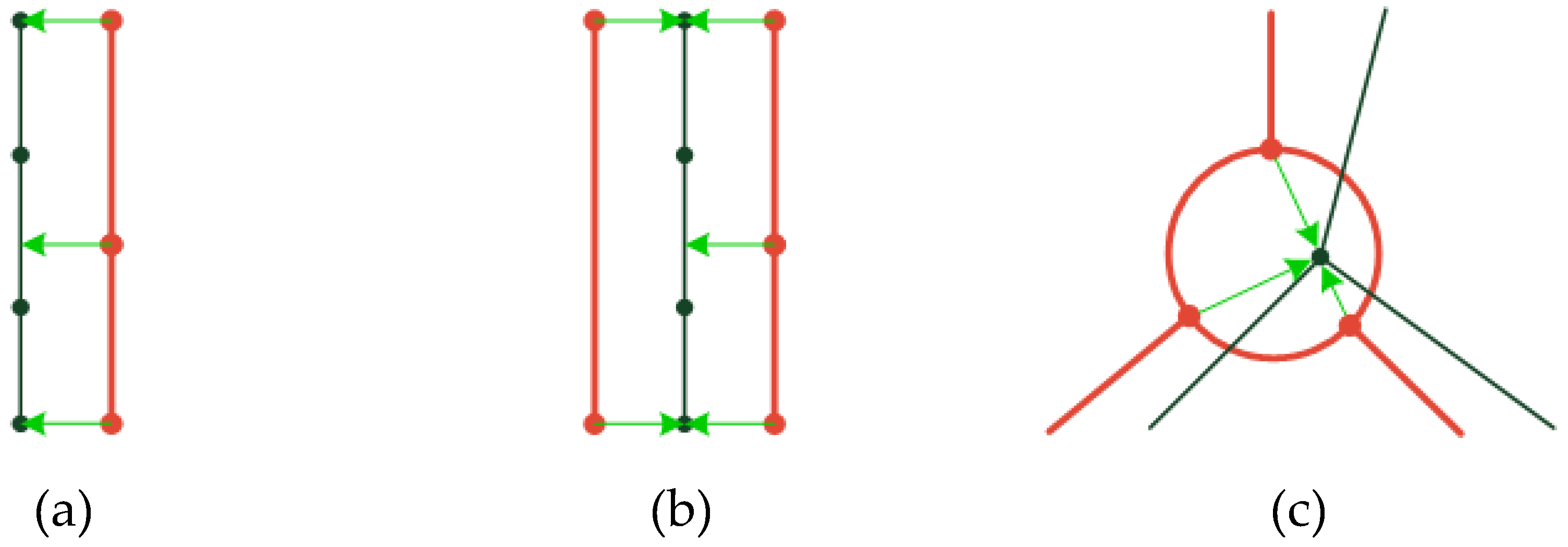
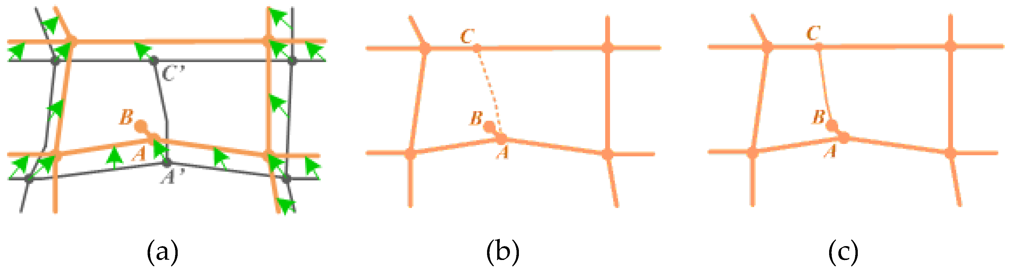
Step 1: Establishment of the control point pairs

A control point pair (abbreviated as CPP) consists of a point in one dataset and a corresponding point in the other dataset. Finding proper control point pairs is an important step in the transformation process as all the other points are aligned based on them (Chen 2005). Essentially, based on the identified matching pairs, the control point pairs can be generated by means of interpolation (ref. Step 2). The identified corresponding coordinates (see the example of green arrows in Figure 3) are stored in the physical memory and act as control point pairs in the next step of “Alignment based on control point pairs”. Here, the control point pair is constructed by the fromPoint in ATKIS (appended dataset) and toPoint in NAVTEQ (reference dataset) which tend to represent the same position in the real world.

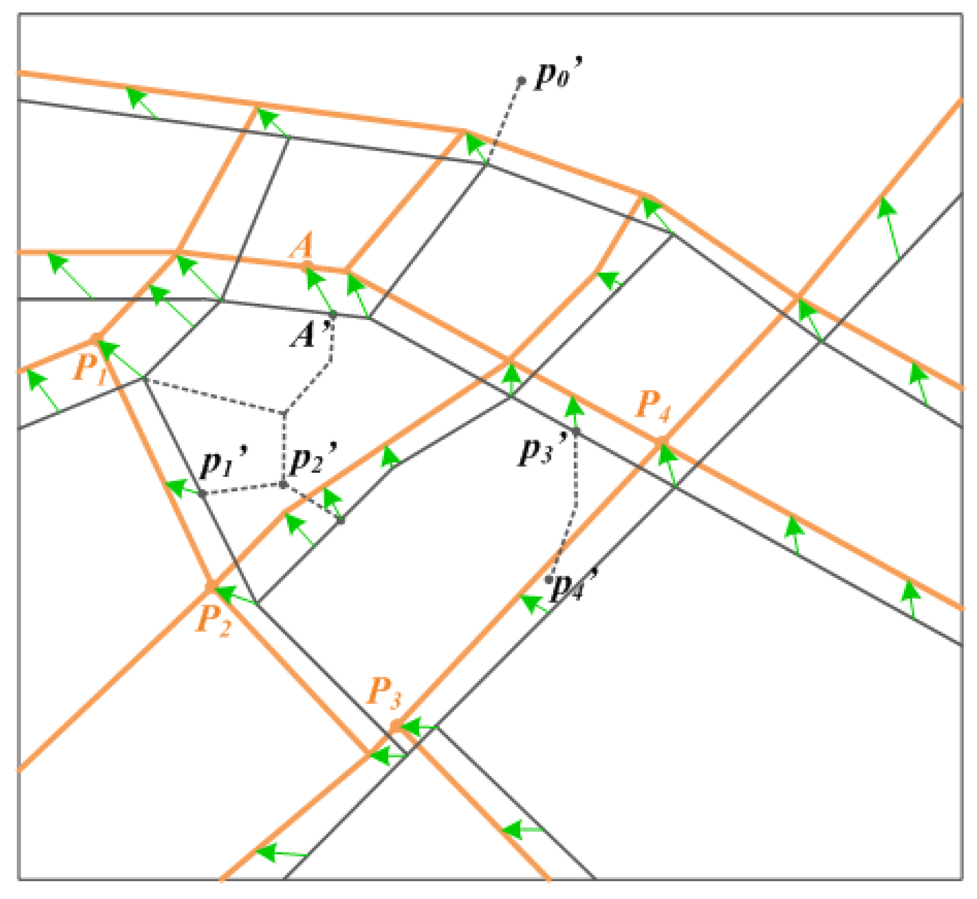
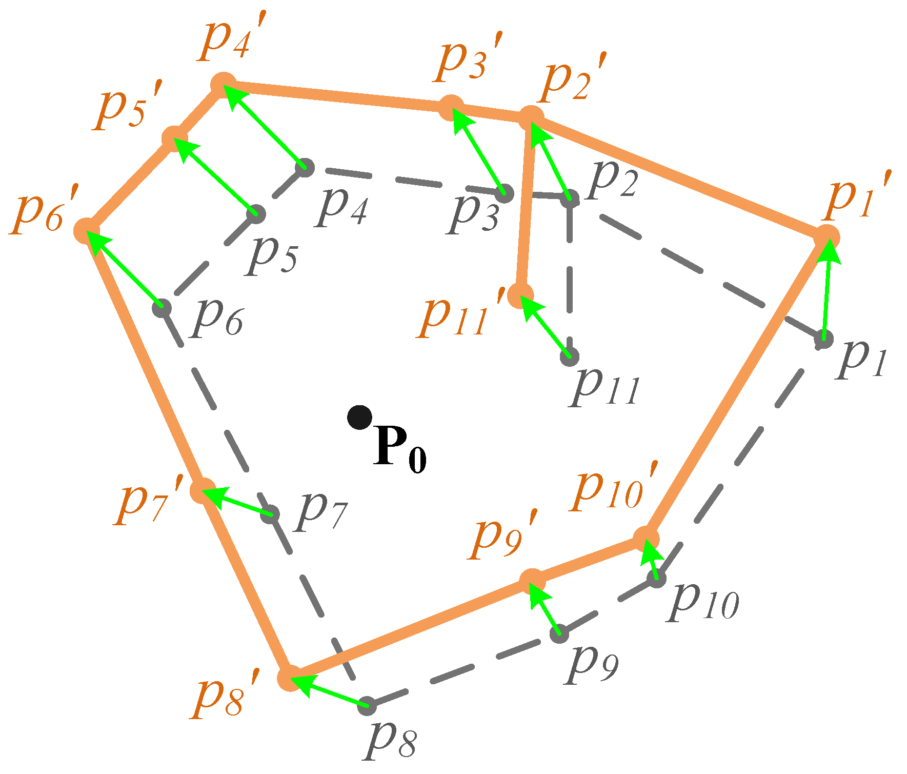
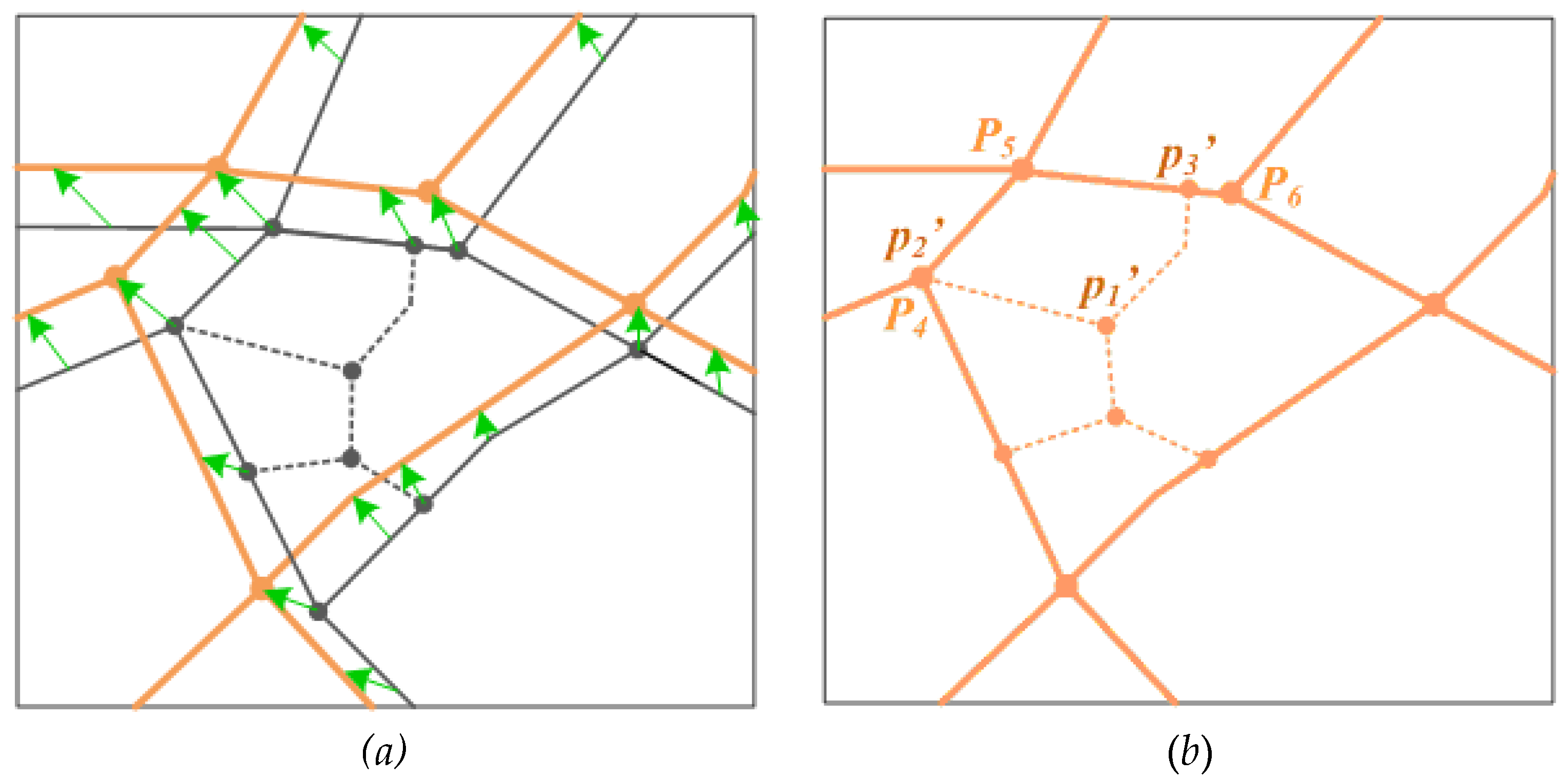
Step 2: Alignment based on control point pairs

The overall transformation of the PWs-tbc from ATKIS needs to satisfy several cartographic constraints, such as preservation of the orientation, the relative spatial position, and the continuity between adjacent objects. This means the turning points of the PWs-tbc should be properly aligned on the basis of the control point pairs (CPPs). According to the topologic characteristics and their relationship to the CPPs, these turning points can be categorized into three groups, (a) Turning points which are duplicated to the fromPoints of CPPs; (b) Road crossings (valence ≥3) or dead-ends (valence =1) which are not duplicated to the fromPoint of any CPP; and (c) Other shape-points along the PWs-tbc. Different categories will call upon different methodologies for the point alignment.
  • (a) Turning points which are duplicated to the fromPoints of CPPs
For this kind of turning point, the alignment is conducted by displacing the turning point between the control point pair, e.g., from the point A’ to A in Figure 3. Such an alignment preserves the topologic continuity and assures that the transformation can sew together joined road objects between diverse datasets.
  • (b) Road crossings or dead ends which are not duplicated to the fromPoint of any CPP
The established control point pairs in step 1 form a distortion map for the whole conflation area. In order to properly adjust the position of the crossings (valence ≥ 3) and dead ends (valence = 1) of the PWs-tbc which are not duplicated to the fromPoint of any CPP, e.g., the nodes p2′ and p4′ in Figure 3, the local transformation is applied, which employs space partition of the whole conflation area into much smaller regions and therefore can better handle the local distortions in each region.
In a road network, the linear topologic structure provides a natural way to spatially subdivide the datasets, i.e., mesh-based partition [21]. A mesh, also called face, can be regarded as a closed region that does not contain any other region. The meshes, e.g., { m e s h i   |   i = 1 ,   2 ,   3 ,   ,   13 } based on the road network of NAVTEQ depicted in Figure 4a, define boundaries in a natural way and also form the zones that separate the objects insides the zones from those outside. Considering that this process aims at transforming the PWs-tbc from the ATKIS, the meshes of { m e s h i   |   i = 1 ,   2 ,   3 ,   ,   13 } based on NAVTEQ have to be distorted around the CCPs. As the result, a set of new meshes { M e s h i   ' |   i = 1 ,   2 ,   3 ,   ,   13 } (see Figure 4b) will be established, which fit the geometries of the dataset of ATKIS.
With each distorted mesh (see examples in Figure 4b), the CCPs can build up a local distortion map, which influences the alignment of the points within or on the boundary of this mesh. Let us define the CPP as vector, where P i = ( X i , Y i ) T is the fromPoint and P i ' = ( X i ' , Y i ' ) T is the endpoint; the neighbor of P i is denoted as P i , j . The concept of “neighbor” can be illustrated by the example in Figure 5, where the point p 2 has three neighbors of { p 2 , 1 , p 2 , 2 , p 2 , 3 |   p 2 , 1 = p 3 , p 2 , 2 = p 1 , p 2 , 3 = p 11 } ; point p 1 has two neighbors of p 1 , 1 = p 2 and p 1 , 2 = p 10 ; and point p 11 has only one neighbor p 2 .
Thus, given a road crossings or dead ends P 0 = ( X 0 , Y 0 ) T falling inside the distorted mesh (see the example of polygon p1p2…p10p1 in Figure 5, its new position P 0 ' = ( X 0 ' , Y 0 ' ) T in the conflated dataset can be calculated by Equation (1).
P 0 ' = P 0 + i = 1 n [ j = 1 m ( p i , j p i ) Τ ( p i , j p i ) ] α [ ( P 0 p i ) Τ ( P 0 p i ) ] β ( p i ' p i ) i = 1 n [ j = 1 m ( p i , j p i ) Τ ( p i , j p i ) ] α [ ( P 0 p i ) Τ ( P 0 p i ) ] β
where,
  • m—number of the neighbors of pi;
  • n—number of the CPPs;
  • α, β—two experimental coefficients larger than 0.
Equation (1) demonstrates that when a given point is duplicated to one of the reference vertexes, the weight of this vertex [ ( P 0 p i ) ] T ( P 0 p i ) ] β approaches infinity. It indicates that the transformation of the given point will be calculated only according to the vertex’s own displacement, which is in accordance with the alignment of the turning points in Group (a) and therefore can provide us a consecutive transformation model.
In practice, the set of CPPs includes more points than those forming closed meshes. It is common to encounter open-end edges or edges that link meshes, which indicate several crossings or dead ends of the PWs-tbc could be outside all of the closed meshes (see point p0’ in Figure 3). For such cases, the proposed local transformation model will build up a well-defined buffer around the given point; then all the CPPs that fall inside this buffer will be taken into account for the transformation; however, if there is no CPP falling inside, the point will keep its initial position after the data conflation.
In order to enhance the computing efficiency, the alignment of the crossings and dead ends in this group could be ignored if the overall geometric deviation between different datasets is small enough (e.g., <3 m).
  • (c) Other Turning points of the PWs-tbc.
The turning points in this group are (i) neither road crossings nor dead end; and (ii) not duplicated to the fromPoint of any CPP. In order to preserve the initial orientation and form of the PWs-tbc, these turning points are aligned based on the point transformations in Group (a) and Group (b). For example, the PWs-tbc p1p2…pn-1pn is restricted by p1 and pn, where P 1 = ( x 1 , y 1 ) T is a turning point in Group (a) with the transformation T p 1 = ( x 1 ,   y 1 ) T   and P n = ( x n , y n ) T is a road crossing in Group (b) with the transformation T p n = ( x n ,   y n ) T . Then, the transformation of the turning point p i   ( 2 i n 1 ) can be calculated by Equation (2), where T p i represents the transformation of the turning point p i and γ is an experimental coefficient between (0,1).
Δ T p i = ( Δ x i , Δ y i ) T = Δ T p n [ ( p i p 1 ) T ( p i p 1 ) ] γ + Δ T p 1 [ ( p i p n ) T ( p i p n ) ] γ [ ( p i p 1 ) T ( p i p 1 ) ] γ + [ ( p i p n ) T ( p i p n ) ] γ ( 2 i n 1 )
After the alignment of all the turning points in Group (a), (b), and (c), the PWs-tbc will have their new forms and positions in the conflated road network (ref. Figure 6).

3.4. Remodelling of the Conflated Dataset

In the conflated dataset, the newly appended PWs-tbc and the initial road network of NAVTEQ should be well organized from both topologic and semantic perspective. To demonstrate this issue, several changed representations in the conflated dataset are discussed in the following subsections.

3.4.1. Creating New Intersections (Nodes)

After the adaptive geometric transformation, one PW-tbc is able to be aligned to the new coincident position in the conflated road network. Topologically, the PW-tbc will have nothing to do with the conflated road network if it is totally apart from the initial road network of NAVTEQ or its touching point to the road network of NAVTEQ is an existing node, see example of the conflated road p1′ → p2′ in Figure 6. The condition, however, becomes more complicated when the PW-tbc touches one road object from road network of NAVTEQ and the touching point is neither from-node nor to-node of this object. In such cases, the conflated road network requires new intersections (nodes) to rearrange the topologies of the conflated road network. For example in Figure 6, the conflation of the PW-tbc p1′ → p3′ necessitates a new intersection p3′ to split the object P5P6 into two parts, which reserves the connectivity between the PWs-tbc and the road network from NAVTEQ.

3.4.2. Decomposition and Transferring of Semantic Information

The decomposition and transferring of the attributes from the reference dataset into the new one is an important function for the map conflation. This is a straightforward task for topologically unchanged road objects because these objects will lead to 1:1 attribute transferring. However, difficulties may occur for those that have been divided by new created intersections, e.g., in Figure 6, the road object P5P6 from the initial road network of NAVTEQ has been split into two objects P5p3′ and p3′ → P6 in the conflated dataset. In this case, the initial attribute of the object should be first decomposed and then transferred to the split parts. The non-spatial attributes of the original object, such as street name, Functional Road Class, Form of Way, etc. can be directly assigned to the newly generated objects, whereas the spatial attributes, such as the street length and travel time, should be fairly assigned to the new ones by means of interpolation.

3.4.3. Entity ID Issues

In the routing capable geospatial database, each geographic entity should have a unique identifier (ID) to distinguish it from all other geographic entities. In general, either object ID or node ID can be concerned for routing purposes.
For the conflated objects, e.g., p1′ → p2′ and p1′ → p3′ in Figure 6, we should assign new object IDs for them. Meanwhile, the node ID of P4 in NAVTEQ is transferred to the to-node of the object p1′ → p2′ (viz. p2′); while new node IDs are required by the nodes which are either initial from the ATKIS (e.g., p1′ in Figure 6) or newly created intersections (e.g., p3′ in Figure 6).
For the unchanged objects from reference dataset of NAVTEQ, e.g., P4P5 in Figure 6, we will keep all the IDs for road object, from-node and to-node. However, if a road object from the reference dataset of NAVTEQ is divided into different parts after the data conflation (e.g., P5P6 in Figure 6), then each part (see P5 → p3 and p3’ → P6 in Figure 6) has to be assigned a new object ID since it acts as an individual road object in the conflated dataset.
Moreover, all of the original object IDs should be reserved to keep the communications between the final conflated dataset and the sources.

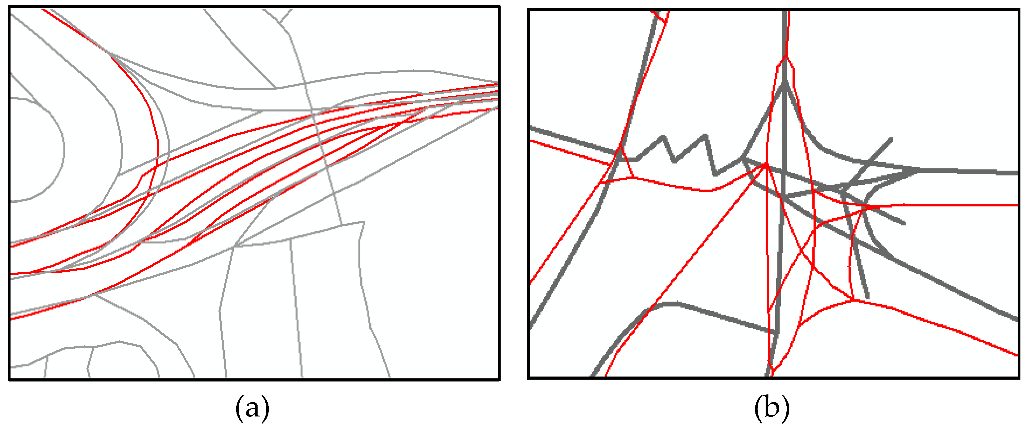
3.5. Error Detection and Correction

Instead of providing comprehensively accurate data conflation between different datasets, the automated routine defined in Section 3.1 to Section 3.4 often leads to an accurate result up to a certain percentage, which indicates that after the automatic data conflation a post-processing is necessary to improve the data quality. Error checking and correction is thereby needed to help the operators to detect and remove/refine the wrongly conflated pedestrian ways. In comparison to the initial road network of NAVTEQ, the conflated pedestrian ways from ATKIS can be classified into four Categories:

Category 1: Duplicated conflated pedestrian ways.

In the proposed approach, the conflated pedestrian ways, which are overlapped or located very closely to the roads from the reference dataset, are regarded as duplications and can be automatically removed from the conflated dataset.

Category 2: Partial duplications.

Figure 7 depicts a very typical instance of partial duplication that could be corrected by the automatic routine: A → C (see Figure 7b) is a conflated pedestrian way which comes from the road network of ATKIS initially (see A’ → C’ in Figure 7a) and A → B is a road stubble from the dataset of NAVTEQ. As the A → B reveals quite different geometries to A’ → C’, e.g., A → B is much shorter than A’ → C’, these two roads have not been matched together by the automatic routine even though they are partially corresponding in reality. Considering that the pedestrian way A → C and the road A → B intersect at point A and angle B A C is small enough, the pedestrian way A → C should be automatically transformed to B → C in the ultimate conflated dataset to avoid the partial duplications (see Figure 7c).

Category 3: Conflated pedestrian ways that are possibly wrong.

The possible wrong conflation refers to the conflated pedestrian ways which are (i) located nearly to the roads from the dataset of NAVTEQ; or (ii) crossing over a road from the dataset of NAVTEQ without any intersection; or (iii) open-ended on both the from-node and to-node of the conflated pedestrian ways, etc. In the proposed approach, interaction tools have been developed to deal with these possibly wrong pedestrian ways. At first, these tools will focus on the possibly wrong conflated pedestrian ways one by one; then the list of all the possible solutions for them will be calculated. Thus, what the human operators have to do is just choose the best solution for error corrections. In this way, the human interaction processes are substantially simplified which leads to an enhancement of working efficiency.

Category 4: Reliable conflated pedestrian ways.

The cases not belonging to Category (1)–(3) can be treated as reliable conflations, which provide very accurate results.

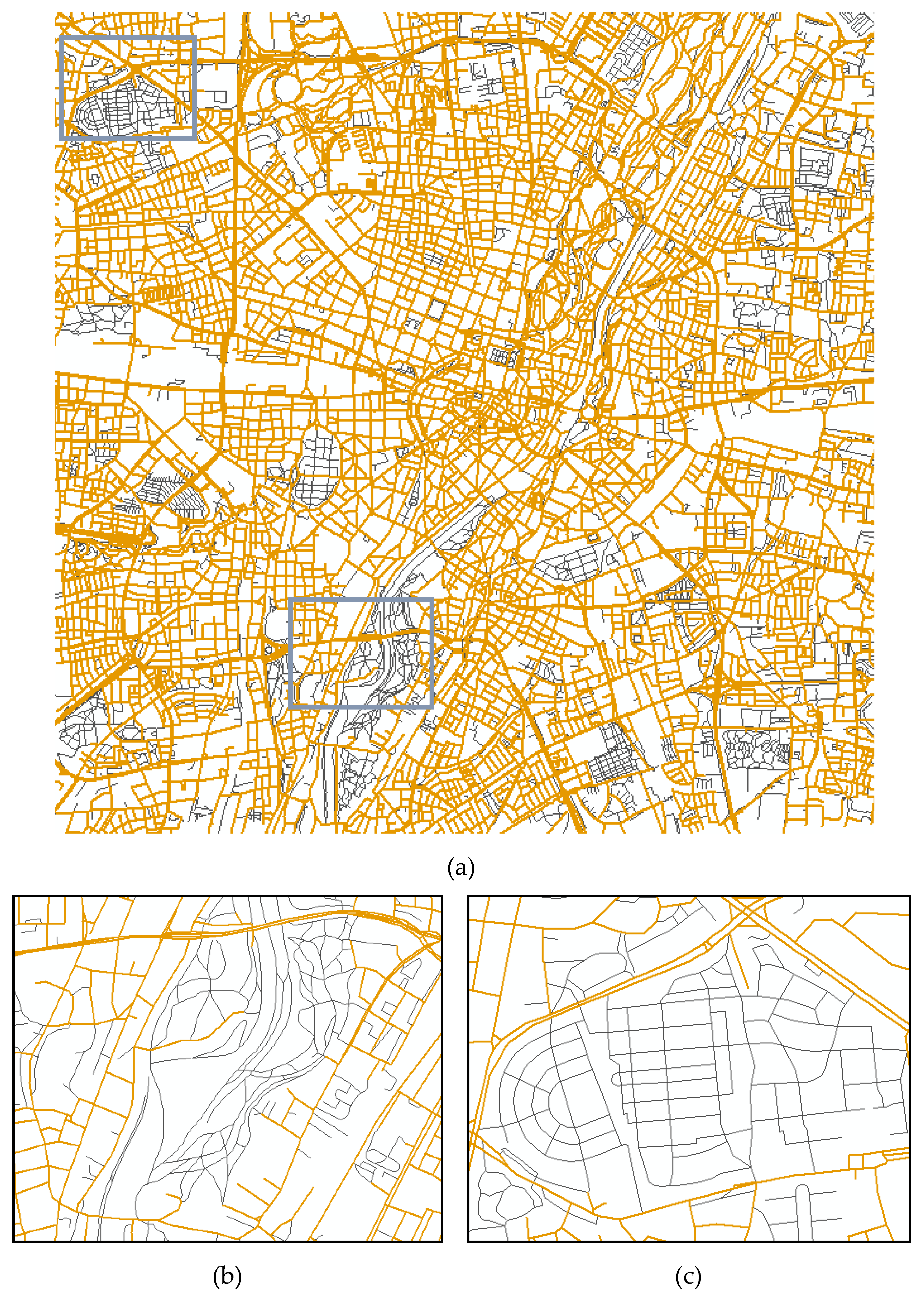
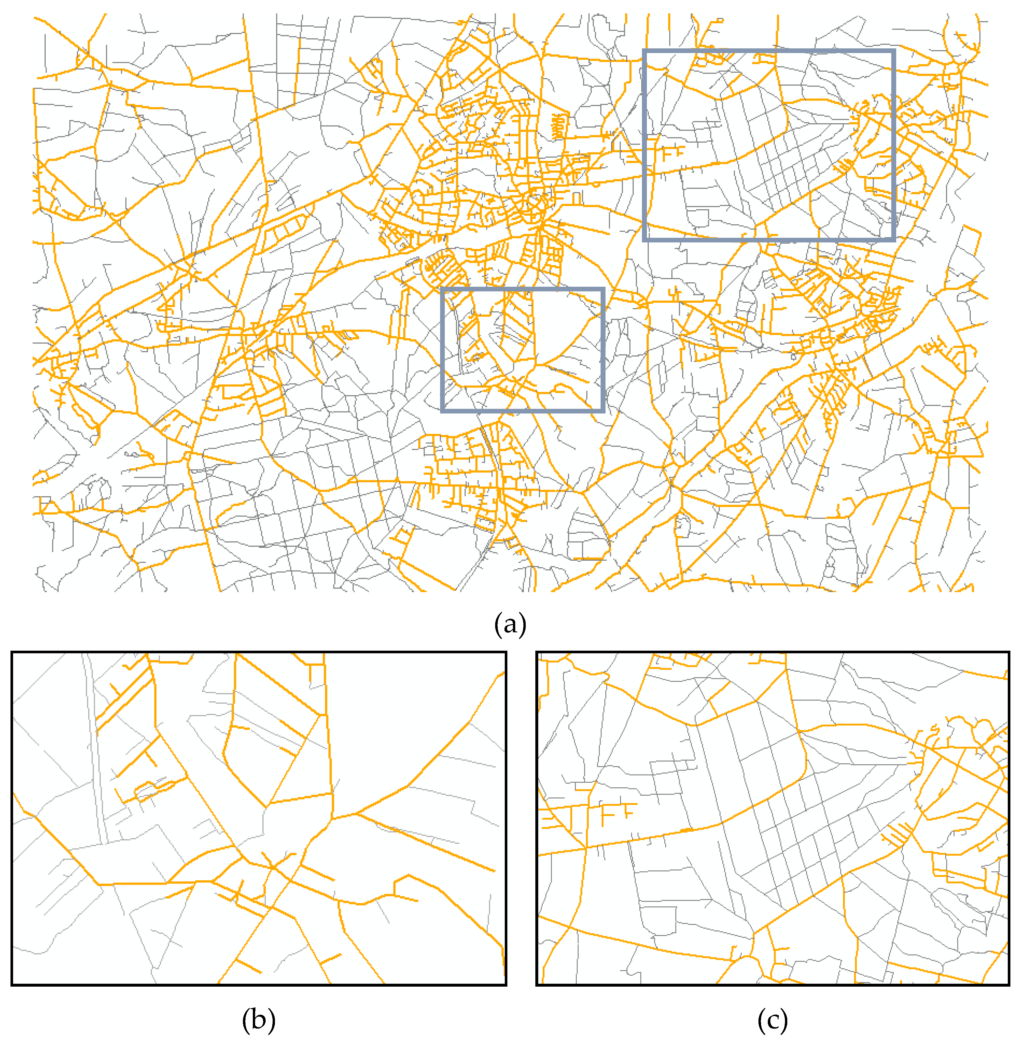
4. Discussion of Conflation Results

As mentioned earlier, the dataset of ATKIS covered many pedestrian ways which were not captured in NAVTEQ. Following the conflation processes defined in this paper, the ATKIS pedestrian ways which do not exist in NAVTEQ can be identified, transformed, remodeled and then appended to the road network of NAVTEQ.
To evaluate the performance of the automatic conflation approach, three examples of the enriched NAVTEQ with additional ATKIS pedestrian ways have been randomly selected in the federal republic of Germany. Here, one is in built-up area of Munich, the others are respectively in rural area of Garmisch and suburbs of Hamburg. As illustrated by Figure 8, Figure 9 and Figure 10, the initial NAVTEQ roads and the appended pedestrian ways from ATKIS have rather consistent position and topologic connection in the conflated road networks, which is very important for routing calculations.
After comparing the automatic conflation results with the manually produced ones, the performance of the proposed approach is evaluated with respect to the measurements of the computing speed and correctness. As demonstrated in Table 1, there are 20,285 NAVTEQ features (reference) and 31,112 ATKIS features; after the automatic conflation, more than 10,000 ATKIS features have been successfully conflated to the reference dataset of NAVTEQ, where only 65 features are conflated either inaccurately or unnecessarily, i.e., this approach revealed satisfactory automatic “correctness” on the conducted experiments. Meanwhile, such a computation is very speedy: to accomplish the three conflation tasks with a total area of ca. 300 km2, it has taken only 39 s in a normal personal computer (Intel Core i7 2.80 GHz).
Obviously, the conflated road network now allows the multi-modal navigations of “driving + walking” due to the fact that (i) it involves both motor roads and pedestrian ways; (ii) the motor roads are fully attributed with the necessary routing-relevant information from NAVTEQ; and (iii) the appended roads do not require so many routing-relevant attributes for navigational purposes since they are prohibited to motor vehicles anyway. Usually the average travel speed on the pedestrian ways can be approximately set as 4 km/hour.
Besides the experiments illustrated in Figure 8, Figure 9 and Figure 10, the proposed conflation approach has been already utilized for real-world data productions on many other large areas in Germany. The overall conflation results are very satisfactory and thereby have been utilized by the GIS and ITS (Intelligent Transportation System) corporations in Germany and Austria (e.g., Alpstein, GeoCOM, Prisma, etc.) as the “data basis” for the development of multi-modal navigation services.
As known, there are two reasons that can lead to imperfections of the automatic data conflation —algorithm limitations and data ambiguity. Within the context of data conflation, the “data ambiguity” refers to the situations when data from different datasets are characterized with geometric/topological conditions that are so complex and/or differentiated that even experienced human operators will have a hard time identifying the correct corresponding counterparts for the proper conflations, see examples in Figure 11. In our experiments, the “data ambiguity” has been confirmed as the primary inducement for many unfavorable conflation results.

5. Conclusions

In this research, the authors have developed an automatic road-network conflation approach for the purpose of transferring the pedestrian ways from ATKIS to NAVTEQ. With 99.79% overall correctness and 99.35% conflation correctness in spite of data complexity and ambiguity, the proposed automatic conflation approach is highly successful. This may come from (a) the high performance of the employed DSO matching algorithm; (b) the hierarchical transformation of the PW-tbc in different categories; and (c) the process of error detection and correction. Besides the conducted experiments, the proposed conflation approach has been implemented in the whole of Germany with a total area of ca. 360,000 km2 and more than 15,388,000 ATKIS objects and 6,690,000 NAVTEQ objects. As a result, the NAVTEQ road-network has been enriched by the appended pedestrian ways from ATKIS and thus gained the necessary capabilities for the development of multi-modal navigation services which have already become basic functionalities in some open platforms (e.g., Google Maps). The same method is now being tested with the data from many other European counties, such as Austria, Switzerland, France, Belgium, The Netherlands, Luxembourg, Denmark, Poland, Czech Republic, etc.
Worth mentioning is also the generic nature of the proposed conflation approach: it can work with the worst case—one or both of the datasets to be matched have no or little semantic information, i.e., it is principally insensitive to the amount of semantic information and thereby can be utilized in the same way for other road-network data models. In fact, the proposed approach has already been implemented for several commercial applications to achieve the comprehensive data conflation among various datasets of Tele Atlas, OpenStreetMap, Swiss Topo, etc. with different application environments. The relevant experiment results will be reported in our subsequent studies. Rather than a significant research prototype, the proposed approach has gained capabilities to be a commercial product.

Acknowledgments

The research described in this article was co-sponsored by (1) National Natural Science Foundation of China as part of the project “Research on the algorithm of multi-sources road-network matching (No. 41301424)”; (2) German Federal Agency for Cartography and Geodesy; and (3) Key Laboratory of Advanced Engineering Surveying of National Administration of Surveying, Mapping and Geoinformation (No. TJES1502).

Author Contributions

Meng Zhang, Wei Yao, and Liqiu Meng conceived and designed the experiments; Meng Zhang performed the experiments; Meng Zhang and Wei Yao analyzed the data; Meng Zhang wrote the paper.

Conflicts of Interest

The authors declare no conflict of interest.

References

  1. Saalfeld, A. Conflation: Automated map compilation. Int. J. Geogr. Inf. Syst. 1988, 2, 217–228. [Google Scholar] [CrossRef]
  2. Chen, C.-C. Automatically and Accurately Conflating Road Vector Data, Street Maps and Orthoimagery. Ph.D. Thesis, University of Southern California, Los Angeles, CA, USA, 2005. [Google Scholar]
  3. Lozano, A.; Storchi, G. Shortest viable hyperpath in multimodal networks. Transp. Res. B Methodol. 2002, 36, 853–874. [Google Scholar] [CrossRef]
  4. Liu, L.; Meng, L. Algorithms of multi-modal route planning based on the concept of switch point. Photogramm. Fernerkund. Geoinform. 2009, 5, 431–444. [Google Scholar] [CrossRef]
  5. Ruiz, J.J.; Ariza, F.J.; Ureña, M.A.; Blázquez, E.B. Digital map conflation: a review of the process and a proposal for classification. Int. J. Geogr. Inf. Sci. 2011, 25, 1439–1466. [Google Scholar] [CrossRef]
  6. Gabay, Y.; Doytsher, Y. Automatic adjustment of line maps. In Proceedings of the GIS/LIS’94 Annual Convention, Phoenix, Arizona, USA, 25–27 October 1994; pp. 333–341.
  7. Gabay, Y.; Doytsher, Y. Automatic feature correction in merging of line maps. In Proceedings of the 1995 ACSM-ASPRS Annual Convention 2, Charlotte, North Carolina, 27 February–2 March 1995; pp. 404–410.
  8. Walter, V.; Fritsch, D. Matching spatial data sets: A statistical approach. Int. J. Geogr. Inf. Sci. 1999, 13, 445–473. [Google Scholar] [CrossRef]
  9. Kang, H. Spatial Data Integration: A Case Study of Map Conflation with Census Bureau and Local Government Data; The Ohio State University: Columbus, OH, USA, 2001. [Google Scholar]
  10. Zhang, M.; Meng, L. An iterative road-matching approach for the integration of postal data. Comput. Environ. Urban Syst. 2007, 31, 598–616. [Google Scholar] [CrossRef]
  11. Zhang, Q.; Griffiths, S.; Wollersheim, M.; Tighe, M.L.; Xu, C. Conflation of national bridge inventory database with tiger based road vectors. In Proceedings of the XXII ISPRS Congress: ISPRS Annals of the Photogrammetry, Remote Sensing and Spatial Information Sciences, Melbourne, Australia, 25 August–1 September 2012.
  12. He, D. A Study on Theory and method of spatial vector data conflation. Res. J. Appl. Sci. Eng. Technol. 2013, 5, 563–567. [Google Scholar]
  13. Zhang, M.; Yao, W.; Meng, L. Enrichment of topographic road database for the purpose of routing and navigation. Int. J. Digit. Earth 2014, 7, 411–431. [Google Scholar] [CrossRef]
  14. Casado, M.L. Some basic mathematical constraints for the geometric conflation problem. In Proceedings of the 7th International Symposium on Spatial Accuracy Assessment in Natural Resources and Environmental Sciences, Lisbon, Portugal, 5–7 July 2006.
  15. Parent, C.; Spaccapietra, S. Database Integration: The Key to Data Interoperability, Advances in Object-Oriented Data Modeling; Papazoglou, M.P., Spaccapietra, S., Tari, Z., Eds.; The MIT Press: Cambridge, MA, USA, 2000. [Google Scholar]
  16. Li, L.; Goodchild, M.F. An optimisation model for linear feature matching in geographical data conflation. Int. J. Image Data Fusion 2011, 2, 309–328. [Google Scholar] [CrossRef]
  17. Volz, S. An iterative approach for matching multiple representations of street data. In Proceedings of the ISPRS Workshop on Multiple Representation and Interoperability of Spatial Data, Hannover, Germany, 22–24 February 2006.
  18. Yang, B.; Zhang, Y.; Luan, X. A probabilistic relaxation approach for matching road networks. Int. J. Geogr. Inf. Sci. 2013, 27, 319–338. [Google Scholar] [CrossRef]
  19. Zhang, M.; Meng, L. Delimited stroke oriented algorithm—Working principle and implementation for the matching of road networks. J. Geogr. Inf. Sci. 2008, 14, 44–53. [Google Scholar] [CrossRef]
  20. Zhang, M.; Meng, L.; Bobrich, J. A road-network matching approach guided by “structure”. Ann. Geogr. Inf. Syst. 2010, 16, 165–176. [Google Scholar] [CrossRef]
  21. Chen, J.; Hu, Y.; Li, Z.; Zhao, R.; Meng, L. Selective omission of road features based on mesh density for automatic map generalization. Int. J. Geogr. Inf. Sci. 2009, 23, 1013–1032. [Google Scholar] [CrossRef]
Figure 1. Strategy to achieve the conflation of different road networks.
Ijgi 05 00068 g001
Figure 2. Identified matching pairs with different matching relationships: (a) m:n matching; (b) Equivalent matching (parallel lines to single line); (c) Equivalent matching (polygon to point). Black lines: road network 1; red lines: road network 2; green arrows: linkages.
Ijgi 05 00068 g002
Figure 3. Matching between NAVTEQ and ATKIS. Orange lines: NAVTEQ; grey lines: ATKIS; dashed lines: pedestrian ways to be conflated (PWs-tbc); green arrows: linkages.
Ijgi 05 00068 g003
Figure 4. Space partition based on meshes: (a) initial meshes based on NAVTEQ; and (b) distorted meshes that fit the geometries of ATKIS. Orange solid lines: initial NAVTEQ; grey dash lines: distorted NAVTEQ; green arrows: linkages.
Ijgi 05 00068 g004
Figure 5. Local distortion map based on mesh partition. Orange solid lines: initial NAVTEQ; grey dash lines: distorted NAVTEQ; green arrows: linkages.
Ijgi 05 00068 g005
Figure 6. Transformation of PWs-tbc from one road network to the other: (a) PWs-tbc before transformation; (b) PWs-tbc after transformation. Orange lines: NAVTEQ; grey lines: ATKIS; dashed lines: conflated pedestrian ways; green arrows: linkages (control point pairs).
Ijgi 05 00068 g006
Figure 7. The process to solve the problems of partial duplications: (a) data matching; (b) data conflation; (c) error correction. Orange lines: NAVTEQ; grey lines: ATKIS; dashed lines: conflated pedestrian ways; dashed lines: conflated pedestrian ways; green arrows: linkages.
Ijgi 05 00068 g007
Figure 8. An example of the conflated road network in a built-up area: (a) a randomly selected area of 10 × 10 km2 in Munich, Germany; (b) partial enlarged view of (a); (c) partial enlarged view of (a). Orange: the initial road network of NAVTEQ; grey: the conflated roads from ATKIS.
Ijgi 05 00068 g008
Figure 9. An example of the conflated road network in a rural area: (a) a randomly selected area of 7 × 7 km2 in Garmisch, Germany; (b) partial enlarged view of (a); (c) partial enlarged view of (a). Orange: the initial road network of NAVTEQ; grey: the conflated roads from ATKIS.
Ijgi 05 00068 g009
Figure 10. An example of the conflated road network in a suburb area: (a) a randomly selected area of 15 × 10 km2 in Hamburg, Germany; (b) partial enlarged view of (a); (c) partial enlarged view of (a). Orange: the initial road network of NAVTEQ; grey: the conflated roads from ATKIS.
Ijgi 05 00068 g010
Figure 11. Examples of “data ambiguity”: (a) an area where the geometric/topologic conditions are very complex; (b) an area where the geometric/topologic conditions are distinct to each other. Red lines: NAVTEQ; grey lines: ATKIS.
Ijgi 05 00068 g011
Table 1. Statistical results of the road-network conflation.
Test Area (km2)Area 1 (100 km2)Area 2 (49 km2)Area 3 (150 km2)Total
NAVTEQ Features (NF)14,9602214311120,285
ATKIS Features (AF)19,5165196640031,112
Conflated Features (CF)51772246259910,022
Unfavorable Conflated Features (UCF)42111265
Computing Time (second) (incl. data reading and writing)25 s6 s8 s39 s
Configuration of the ComputerIntel Core i7 2.80 GHz
Correctness
Overall Correctness = (AF − UCF)/AF × 100%99.78%99.79%99.81%99.79%
Conflation Correctness = (CF − UCF)/CF × 100%99.19%99.51%99.54%99.35%

