Coastline Zones Identification and 3D Coastal Mapping Using UAV Spatial Data

Abstract

Spatial data acquisition is a critical process for the identification of the coastline and coastal zones for scientists involved in the study of coastal morphology. The availability of very high-resolution digital surface models (DSMs) and orthophoto maps is of increasing interest to all scientists, especially those monitoring small variations in the earth’s surface, such as coastline morphology. In this article, we present a methodology to acquire and process high resolution data for coastal zones acquired by a vertical take off and landing (VTOL) unmanned aerial vehicle (UAV) attached to a small commercial camera. The proposed methodology integrated computer vision algorithms for 3D representation with image processing techniques for analysis. The computer vision algorithms used the structure from motion (SfM) approach while the image processing techniques used the geographic object-based image analysis (GEOBIA) with fuzzy classification. The SfM pipeline was used to construct the DSMs and orthophotos with a measurement precision in the order of centimeters. Consequently, GEOBIA was used to create objects by grouping pixels that had the same spectral characteristics together and extracting statistical features from them. The objects produced were classified by fuzzy classification using the statistical features as input. The classification output classes included beach composition (sand, rubble, and rocks) and sub-surface classes (seagrass, sand, algae, and rocks). The methodology was applied to two case studies of coastal areas with different compositions: a sandy beach with a large face and a rubble beach with a small face. Both are threatened by beach erosion and have been degraded by the action of sea storms. Results show that the coastline, which is the low limit of the swash zone, was detected successfully by both the 3D representations and the image classifications. Furthermore, several traces representing previous sea states were successfully recognized in the case of the sandy beach, while the erosion and beach crests were detected in the case of the rubble beach. The achieved level of detail of the 3D representations revealed new beach characteristics, including erosion crests, berm zones, and sand dunes. In conclusion, the UAV SfM workflow provides information in a spatial resolution that permits the study of coastal changes with confidence and provides accurate 3D visualizations of the beach zones, even for areas with complex topography. The overall results show that the presented methodology is a robust tool for the classification, 3D visualization, and mapping of coastal morphology.

1. Introduction

Coastal zone monitoring is an important task in environmental protection, while coastline detection is fundamental for coastal management [1]. Coastal management requires up-to-date accurate information since coastal movements are of primary importance in evaluating coastal erosion. Remote sensing plays a significant role in coastal observation as it is one of the most valuable tools used for detecting and monitoring coastlines. The scope of this paper is to detect the coastline and to identify the coastline zones by applying geographic object-based image analysis (GEOBIA) to high-resolution orthophotos produced by an unmanned aerial vehicle (UAV) combined with a structure from motion (SfM) algorithm, and to reconstruct the study areas in a three-dimensional (3D) representation to examine if other beach characteristics, such as swash zones, wrack lines, and berm zones, can be identified.

Although the spatial resolution of satellite imagery has significantly improved in the last decade, the data collected is still not sufficient for medium to small coastal changes (centimetric accuracy). Conversely, UAVs in combination with SfM, which is also called a UAV-SfM pipeline, can provide high-resolution information at a low cost for a small area [2,3]. The miniaturization of sensors and the increase in the flight capabilities and agility of UAVs, as well as the high-quality imagery tools that are available have combined to produce a spatial data acquisition tool for environmental monitoring [4,5,6]. Several recent publications have described methods and techniques that measure changes in coastal morphology zones using UAVs [4,7,8]. Currently, UAVs are a viable option for collecting remote sensing data for a wide range of practical applications, including scientific, agricultural and environmental applications [4,6,8,9,10,11,12,13,14,15,16,17,18] Unmanned aerial systems (UAS), which consist of a UAV and a sensor, provide digital images with spatial and temporal resolutions that are capable of overcoming some of the limitations of spatial data acquisition using satellites and airplanes. The resolution of the data commonly available using conventional platforms, such as satellites and manned aircraft, is typically in the range of 20 to 50 ${\displaystyle \frac{cm}{pixel}}$ [19]. For example, the acquired spatial data resolution via a manned aircraft ranges from 10-100 cm when the satellite system provides a resolution greater than 50 cm [12].

Datasets produced by UAV-based remote sensing have such a high spatial resolution (2–5 cm) that characteristics and changes of the landscape, such as coastal morphology, coastal zones, and beach morphological characteristics, can be mapped in detail in two (2D) and three dimensions (3D) [3,8,20,21]. However, such small changes are not distinguishable at the spatial resolutions generally obtained using manned aircraft and satellite systems. Furthermore, the high level of automation, the ease of deployment, the ease of survey repeatability, and the low running costs of UAVs in comparison with other traditional remote sensing methods, allows for frequent missions that provide spatial datasets with a resolution of less than 5 cm and a high temporal repetition due to the ease of survey deployment [12,22,23]. Georeferenced orthophotos and digital surface models (DSMs) are used to measure and depict the morphology of a beach in 2D and 3D, which allows the assessment of changes to the beach due to extreme wave phenomena [6].

Recent advances in computer vision include SfM algorithms, which have been successfully used for the reconstruction of large uncontrolled photo collections [24,25,26]. Studies have described the adaptation of SfM techniques to process UAV data photography to create an accurate georeferenced 3D point cloud and to generate a high-resolution DSM; SfM techniques have also been used in the orthorectification of georeferenced images that have been joined together to form a mosaic [6,19].

Hay and Castilla stated in 2008 that geographic object-based image analysis (GEOBIA) is a new discipline that involves the object-based analysis of Earth’s surface using remote sensing imagery. They defined GEOBIA as “as a sub-discipline of Geographic Information Science (GIScience) devoted to developing automated methods to partition remote sensing imagery into meaningful image-objects, and assessing their characteristics through spatial, spectral and temporal scales, so as to generate new geographic information in GIS-ready format” [27]. Using GEOBIA for coastline zone extraction involves exporting the geographic information in vector format with the classes of water and beach zones assigned through an automatic procedure [28].

The present work uses the UAV-SfM pipeline for spatial data acquisition, high-resolution geoinformation production, and 3D visualization of coastal morphology assisted by GEOBIA for the identification of coastal zones. More specifically, the proposed methodology uses GEOBIA of high-resolution orthophotos for the definition of coastal zones. The combination of these innovative techniques is applied in two diverse coastal areas to examine the efficiency of the developed method.

The potential use of the UAV-SfM pipeline has been evaluated in several studies [5,6,8,19,29]. However, references about the use of GEOBIA with the geographic information produced by the UAV-SfM methodology for coastal monitoring are still scarce in the recent scientific bibliography.

A coastline is defined as the line that forms the boundary between the land and the sea; the detection of a coastline in high resolution includes recognizing several discontinuities [30,31]. However, the boundary between water and land is not easily distinguishable in clear water. For the proper study of coastal areas, the four typical beach zones should be examined. These beach zones include the swash zone, beach face, wrack line, and berm. The swash zone is the area of land that is alternately covered by the sea or exposed to wave runup. The beach face includes the sloping section of land that is exposed to the swash of the waves. The wrack line is the highest reach of the daily tide. The berm is the area of land that is almost horizontal; it is the dry portion of the coast that usually contains sand dunes.

2. Materials and Methods

The goal of our surveys was to generate an accurate orthophoto and 3D model of the case study area to detect and to visualize the coastline in both Eressos and Neapolis coastline systems. In this study, our main surveying device was a quad-copter UAV for the acquisition of high-resolution aerial images of the two study areas. These images were used for the GEOBIA coastline zone identification and 3D modelling of the coastal morphology.

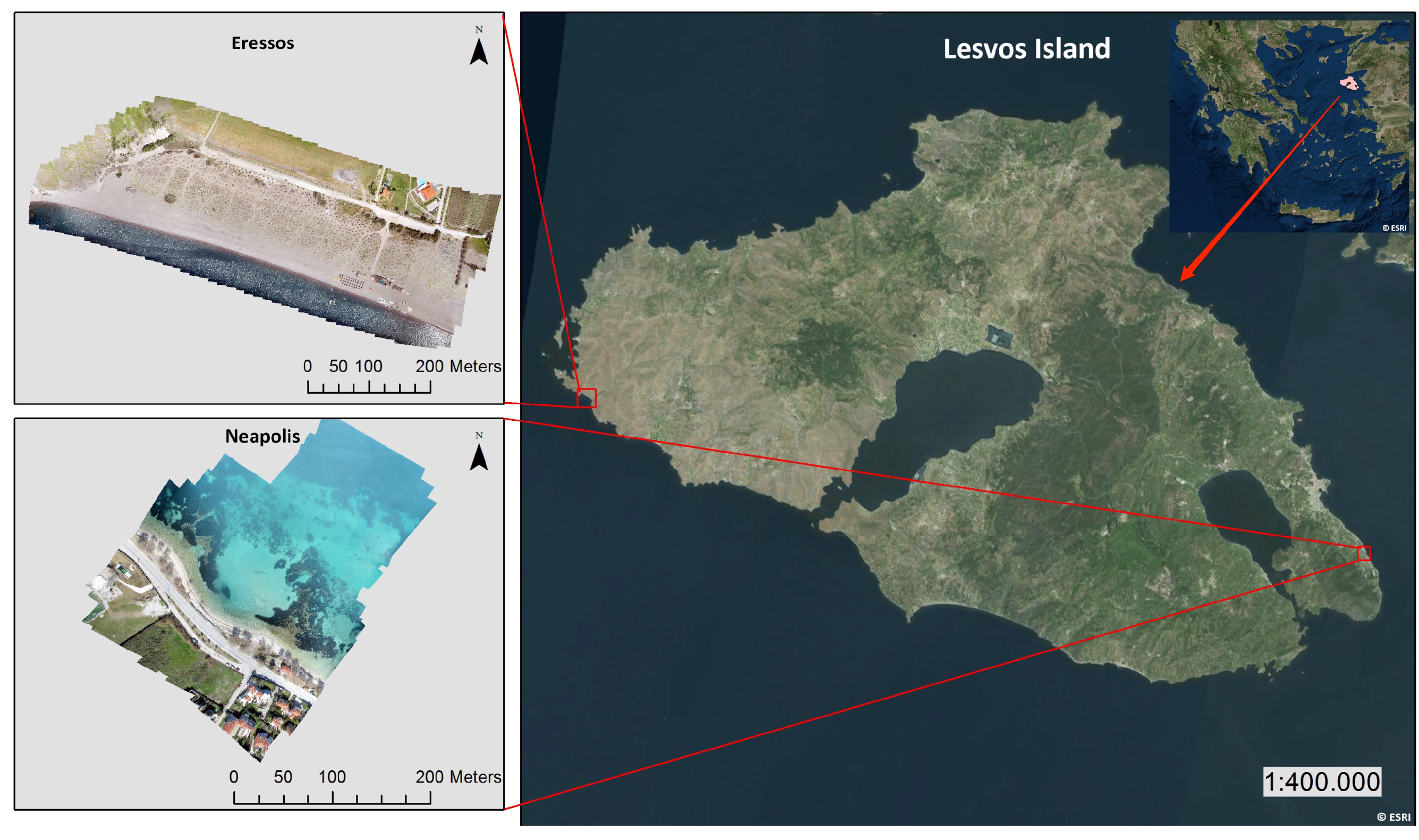
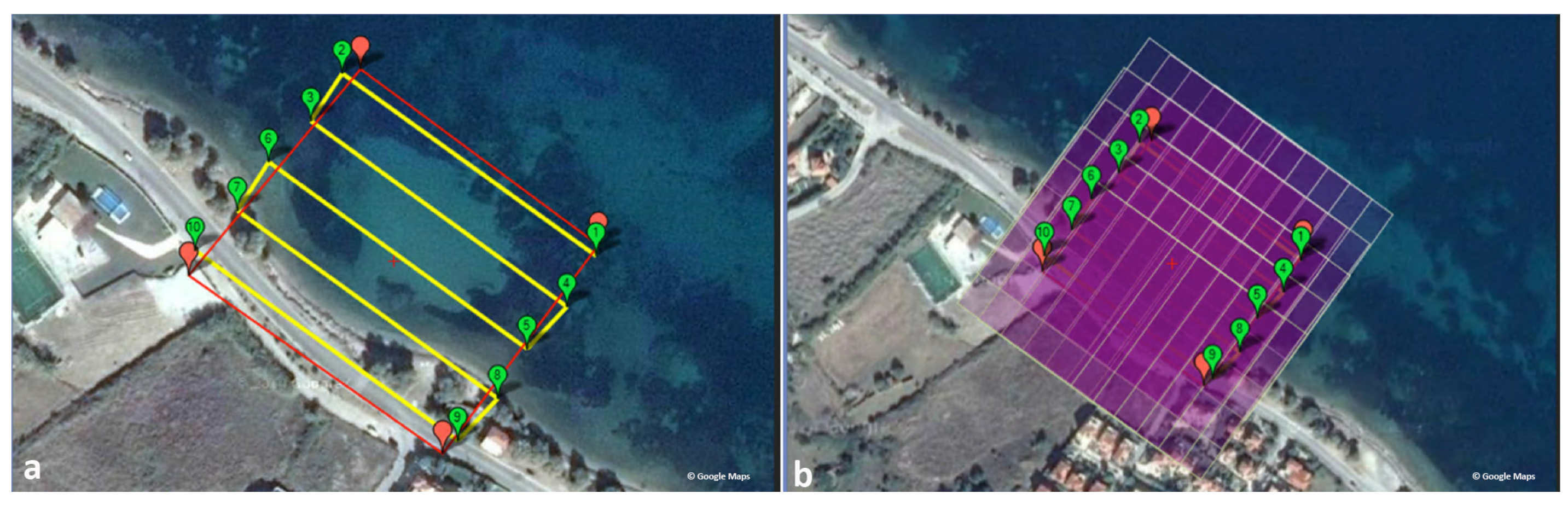
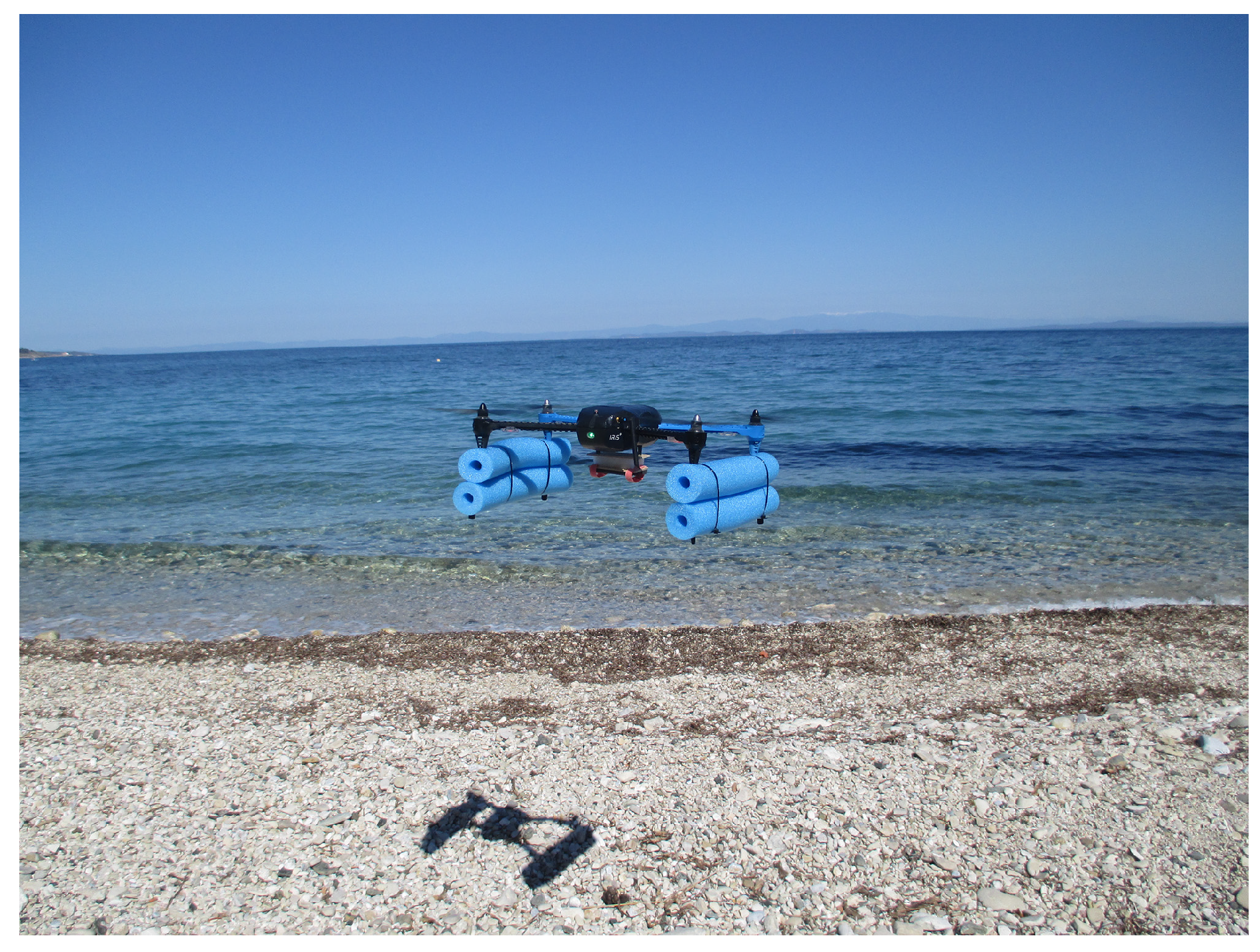
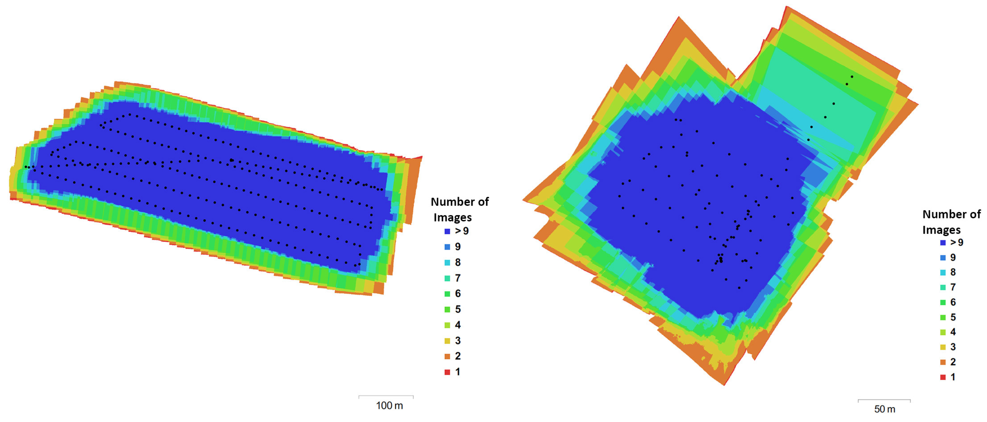
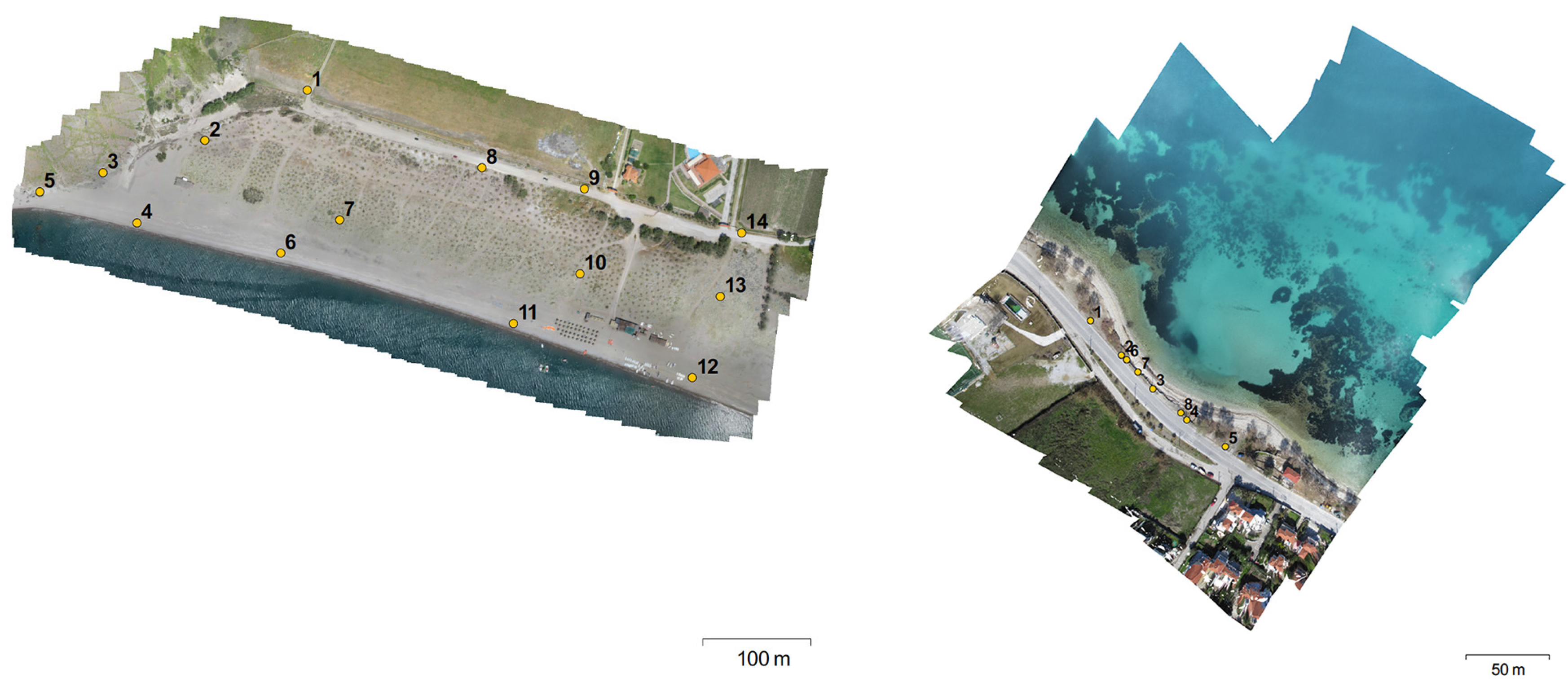
2.1. UAV System Data Collection

The UAV system used a vertical take off and landing (VTOL) configuration that was capable of performing programmed GPS missions with waypoints, as well as fully autonomous flight missions (Figure 1). The main parts of the airborne system included the airframe, motors, actuator power supply that was powered by brushless motors, and lithium polymer batteries. The UAV configuration consisted of a Pixhawk autopilot system that controlled the sensor fusion and the current flight information; a 3DR uBlox GPS with Compass module; a STMicroelectronics L3GD20 3-axis 16-bit gyroscope; a STMicroelectronics LSM303D 3-axis 14-bit accelerometer/magnetometer; a MPU 6000 3-axis accelerometer/gyroscope; a MEAS MS5611 barometer; and 3DR ground station telemetry radios. The take off payload capacity of the UAV was 0.4 kg and the flight time was approximately 15 min. Additionally, a remote control was used for sending commands within the 2.4 GHz frequency band to be subsequently processed by the flight control board. The bidirectional telemetry worked within the 433 MHz provided by the radio links and allowed the ground station computer to wirelessly communicate with the quad-copter. The Canon ELPH 130 with 16 Mpixel (4608 by 3456 pixels) sensor was chosen as the survey camera because of its lightweight, manual functions, and programming capabilities through open source custom software. Figure 2 shows the open source Mission Planner v1.25 software [32] used for monitoring the UAV, as well as for setting up the flight missions. The overall cost of the UAV system, including the sensor (camera), was less than 1000 euro.

Two case study areas were selected in Lesvos Island, Greece; Eressos beach in the southeast and Neapoli beach in the (Figure 2). The sites presented significantly different coastline characteristics, but both are affected by erosion. Eressos beach is a large sandy beach approximately 4 km long that is affected by large north waves. It has a typical profile with a swash zone, a beach face, and a large bern with sand dunes. The southern part of Eressos beach is decreasing in width due to winter storms. In the last decade, the southern part of the beach has lost more than 10 m in width. Neapoli beach is a narrow beach next to a main road network that consists of a mixture of sand and gravel; it also contains dead algae that form a certain line in several areas along the coastline. This beach also contains trees (Tamarix) that help prevent erosion, although they are extremely close to the sea and influence the beach zone recognition. Due to strong north winds during the winter, Neapoli beach is affected by erosion that is represented by the shadows in the orthophoto maps.

The data acquisition was performed in March and April 2015 using a UAS. The missions were planned in two blocks: one for Neapoli beach (Figure 3a) and one for Eressos beach. The average flying height of the UAV was 100 m above ground level (AGL), while the camera was programmed to capture the nadir photograph every 3.5 s with an acquired image footprint of 123.4 m × 91 m (Figure 3b). The captured photos were screened and a subset of 384 clear (not blurred) photos for both areas was selected for the SfM process. The resolution of the images, which is the ground sample distance (GSD), or pixel size, was chosen to be 2.96 cm for both Neapoli beach and Eressos beach. The maximum image size recorded over the test area was 4608 × 3456 pixels; with a pixel size of 1.8 $\mathsf{\mu }{\mathrm{m}}^2$, the GSD was 2.96 cm.

For both case studies, the UAV missions were planned to have an 80% overlap in-track (flight direction) and an 80% cross-track sidelap. Thus, in the study area, most of the points were imaged in nine or more photos. Figure 4 shows the camera positions and the image overlapping for both beaches.

Prior to the survey missions for the two case studies, a team deployed georeferenced mobile targets as ground control points (GCP) in the ground using the RTK-GPS Topcon HiPer II. The targets were placed between the breaker zone and the upper beach with a spatial distribution that is shown in Figure 5. All the targets measured 297 mm × 420 mm (A3 size) and were designed in a black and white pattern, having circles with a 3-cm radius in each target center. This circle represented the center that had to be clearly visible in the image for the correct georeference of the orthophoto and DSM.

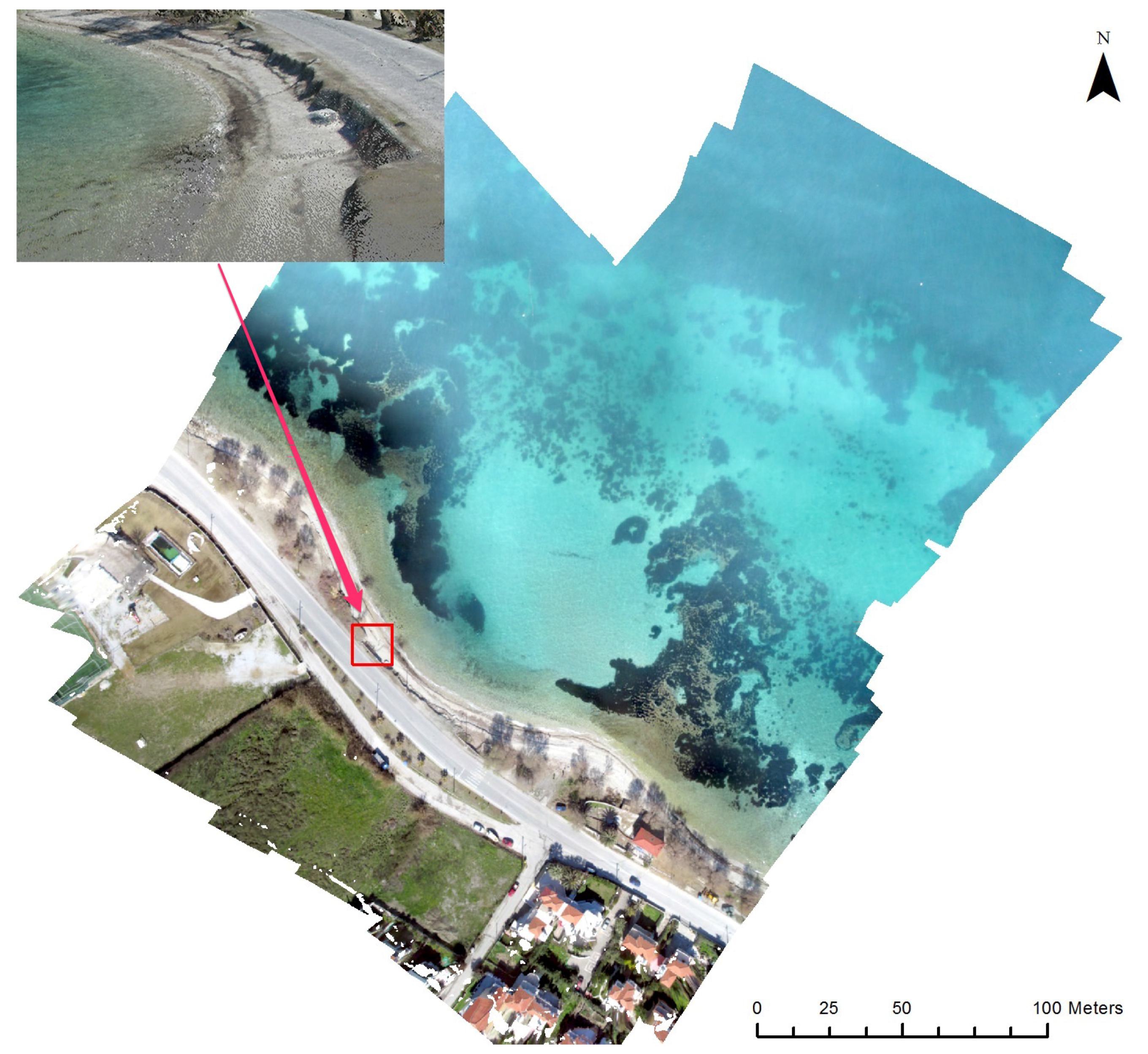
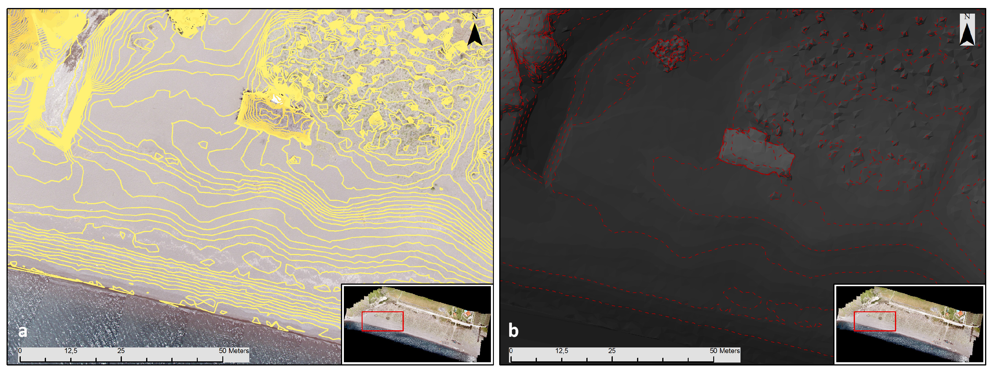
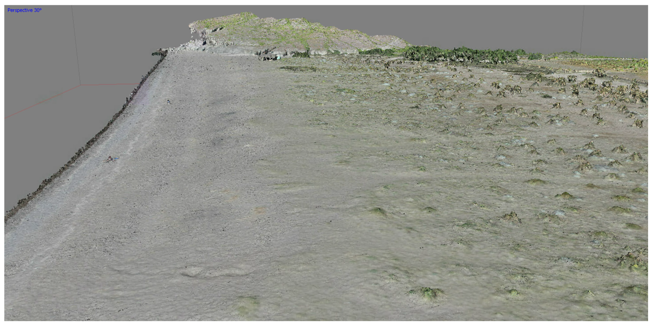
2.2. 3D Visualization and Orthophoto Map Production

Several commercial and non-commercial software packages have been developed to process UAV image data. These software packages bring together computer vision algorithms and conventional photogrammetric methods. These packages use multi-view stereopsis (MVS) technology to produce detailed 2D and 3D geoinformation from UAV-captured unstructured aerial images. We used Agisoft Photoscan [33] because it automates the SfM pipeline in a user-friendly interface with a concrete workflow. Additionally, this software has an error control and functionalities that allow the easy transfer of the produced geoinformation in GIS-readable file formats. In particular, Agisoft was used to detect image feature points in each image and match them with the total of images captured from the UAV system. These matches produced a sparse point cloud as the basis for the generation of the scene geometry as represented by a dense point cloud [8,11,34]. The derivatives produced during the SfM procedure consisted of a set of points, which contained X, Y, Z information, as well as the color information derived from the photographs. These SfM outputs relied on an internal arbitrary coordinate system that had to be transformed to real-world coordinates [29]. The dense 3D point cloud and the total images were used to create a 3D mesh of the scene geometry, high-resolution orthophotos, DSMs, and digital terrain models (DTM) for both study areas.

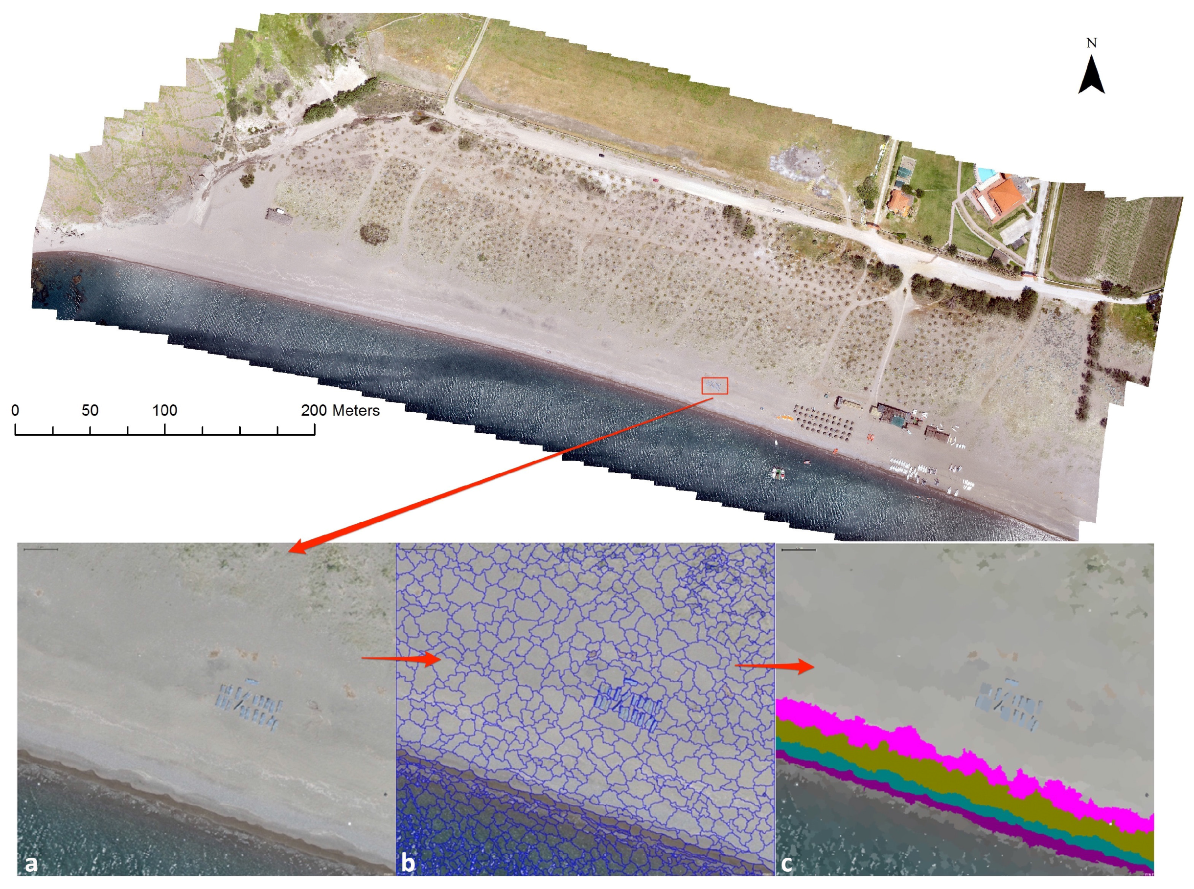
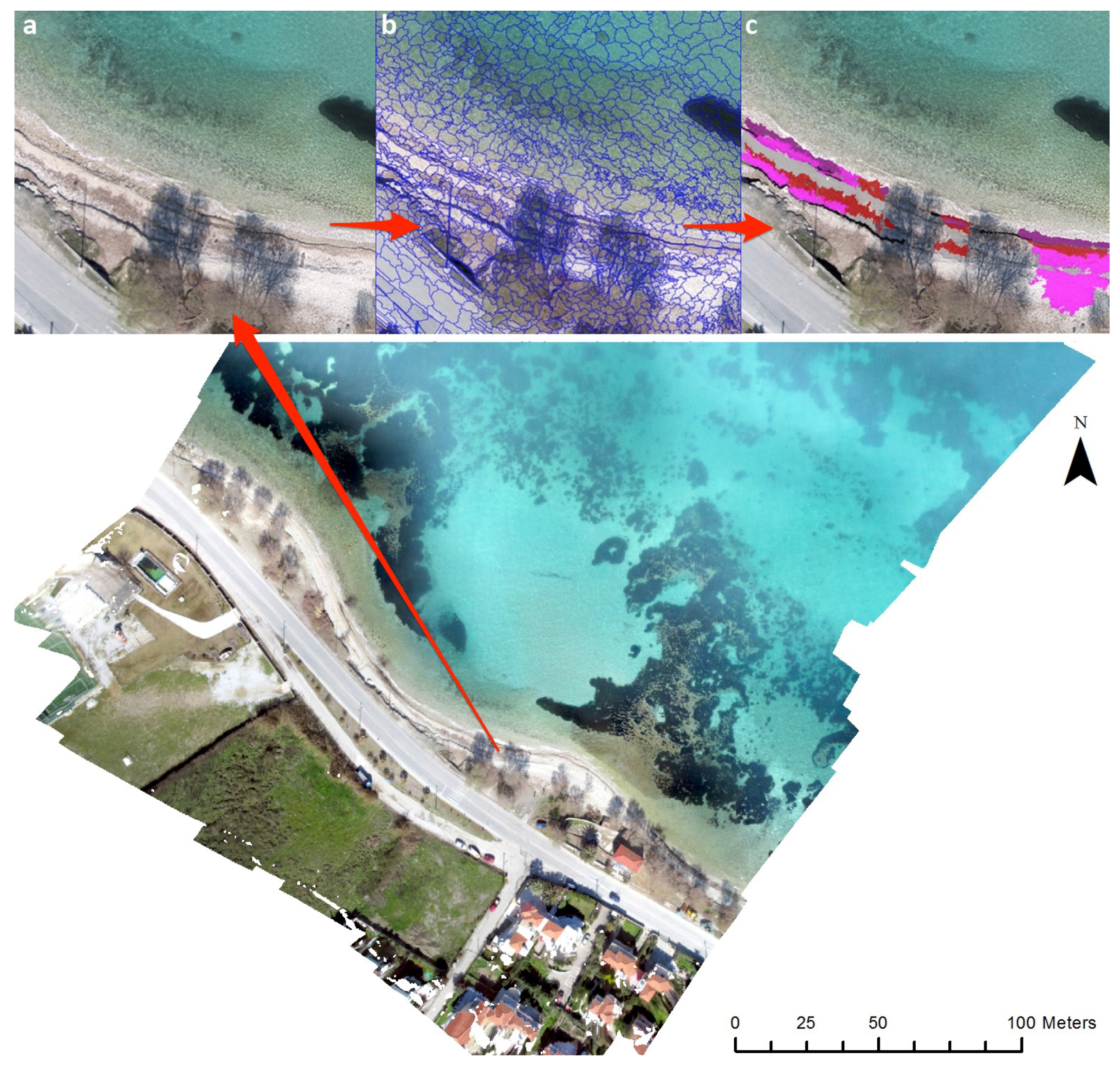
2.3. GEOBIA - Coastline Detection

GEOBIA was used to detect the different beach zones and the coastline. For this analysis, images were segmented into groups of pixels with similar spectral and spatial characteristics. A multiresolution segmentation algorithm that was previously used in several oceanic applications [21,35,36]. eCognition Developer 9.1 software [37] was used with the following multiresolution segmentation parameters: size 20, shape 0.5, and compactness 0.5. The following classes of coastlines were delineated: sea, wet sand, and underwater rocks. Training areas representing those classes were selected in the orthophoto map by visual inspection. At least 50 training sites for each class were used in a stratified random sampling scheme. The selected areas were used to define the spectral shapes and spatial characteristics of each class. Those characteristics were transformed into classification rules with fuzzy logic.

After classification, post processing was done to correct any misclassified objects. At the same time, the coastline was manually digitized in the orthophoto map for comparison. The overall procedure included the following methodological steps: segmentation, class definition, training area selection, rules determination, fuzzy classification, manual coastline determination, and accuracy estimation.

3. Results and Discussion

The UAV-SfM pipeline was performed for Eressos beach and Neapoli beach. All the geoinformation that was produced was referred to the GGRS87 / Greek Grid (EPSG: 2100). The dense point clouds produced for Eressos beach and Neapoli beach consisted of 456.7 and 581.171 ${\displaystyle \frac{point}{m^2}}$, respectively. The accuracy of the geoinformation produced was evaluated by calculating the residuals, the root sum of the squares error (RSSE), and the root mean square errors (RMSE) for all GCPs used in both survey missions. The produced orthophoto pixel resolution was 2.34 and 2.41 ${\displaystyle \frac{cm}{pixel}}$ for Neapoli beach and Eressos beach, respectively. Furthermore, the produced DSM pixel resolution from the Neapoli survey mission was 4.35${\displaystyle \frac{cm}{pixel}}$, while the DSM pixel resolution from the Eressos survey was 4.68 ${\displaystyle \frac{cm}{pixel}}$. The GCPs error statistics for the Eressos survey mission are summarized in

Table 1. GCPs Error Statistics for the Eressos Survey Mission.

	X Error	Y Error (m)	Z Error (m)	RSSE (m)
1	−0.013946	−0.027066	+0.011029	+0.032384
2	−0.014527	−0.064581	+0.041894	+0.078337
3	−0.010834	+0.031295	+0.006176	+0.033688
4	+0.000407	+0.01248	−0.047335	+0.048955
5	−0.013913	+0.003161	+0.003906	+0.014793
6	+0.022724	+0.041989	−0.004675	+0.047972
7	+0.02499	−0.022705	+0.006861	+0.034454
8	+0.038457	+0.072	−0.05524	+0.098561
9	+0.029293	−0.006734	−0.003382	+0.030247
10	−0.03736	−0.037101	+0.055222	+0.076301
11	+0.00587	−0.006312	+0.001308	+0.008719
12	+0.026839	−0.010243	−0.016675	+0.033216
13	−0.016053	−0.028462	+0.029556	+0.044061
14	−0.041859	+0.042076	−0.029186	+0.066139

. The GCPs error statistics for the Neapoli survey mission are presented in

Table 2. GCPs Error Statistics for Neapoli Survey Mission.

	X Error (m)	Y Error (m)	Z Error (m)	RSSE (m)
1	−0.084526	−0.005193	+0.032905	+0.090853
2	−0.007139	+0.049133	−0.039916	+0.063705
3	−0.156592	+0.05385	+0.015161	+0.166285
4	−0.101613	+0.012272	+0.019812	+0.104251
5	−0.012858	+0.030812	−0.011053	+0.035169
6	+0.141038	−0.043869	+0.016315	+0.148602
7	+0.079281	−0.009084	−0.04635	+0.092284
8	+0.139628	−0.091736	+0.016157	+0.167847

. The RSSE for all GCPs in the Eressos survey mission was from 1 to 7 cm; the RSSE for the Neapoli survey mission was found from 3 to 16 cm. The UAV-SfM pipeline accuracy and estimated error for both surveys are summarized in

Table 3. Comparison of error statistics.

Fligh	Ortho GSD	DSM Resolution	X RMSE	Y RMSE	Z RMSE	RSS	RMSE
	(cm/pix)	(cm/pix)	(m)	(m)	(m)	(m)	(pixels)
Eressos	2.34	4.68	0.0408	0.0389	0.00404	0.0565	0.187
Neapolis	2.41	4.15	0.1048	0.0459	0.0276	0.0117	0.585

. The orthophoto and DSM RMSE for both cases was calculated as 0.187 and 0.585 pixels, respectively. The difference in accuracy between the two survey missions is due to the different spatial distribution and the number of GCPs used for georeferencing the orthophoto maps and DSM. These differences could be attributed to the use of 14 GCPs in the Erresos survey compared with the 8 GCPs used in the Neapoli survey. Furthermore, the low quality of the camera lens increased the accuracy error due to high image residuals. However, the achieved accuracy met the requirements for creating highly detailed 2D/3D visualizations and for defining coastal zones, which was the main focus of this study.

The generated orthophoto from the Neapoli study site had a resolution of 2.41 cm (Figure 6). The inset in Figure 6 illustrates the swash zone, wrack lines, and berm zone in 3D. The level of detail of the generated 3D visualizations clearly shows the structure of the coastal zones. Additionally, the DSM produced by the workflow presented in this paper had a spatial resolution of $\le 5$ cm for both beaches. Figure 7 shows the orthophoto and dsm for Eressos beach.

Figure 6, Figure 7 and Figure 8 show the high degree of detail that was achieved using the UAV-SfM methodology. Aside from the coastline, small variations, such as small rocks and small benches on the beach, are visible over the whole extent of the mapped area (refer to the inset in Figure 6 and Figure 8).

Several important beach characteristics, including the swash zone, beach face, wrack line, and berm, are visible in high-resolution orthophoto maps, but are not visible in high-resolution satellite images. Orthophotomaps cannot be processed using the remote sensing pixel-based classification methodologies (e.g., nearest neighbour) because spectral representatives are similar for the different classes. The segmentation of the orthophoto maps is a critical step since the characteristics of various objects can be used in the classification process. Since the segmentation size, shape, and compactness determine the geometry of an object in the multiresolution segmentation, the characteristics should be carefully assessed. Water clarity and wave state are causes of coastline misclassification. Coastline detection in orthophoto maps with a spatial resolution of centimeters depends on the complexity of the beach. In cases with a simple structure, such as a sand beach with a large face, the detection of the swash zone and beach face can be achieved with high accuracy (Figure 9). However, in complicated cases where the beach is a mixture of composition, such as shingles with various sizes, dead algae, tree shadows, and erosion gaps, the detection of the coastline is more difficult (Figure 10). DSMs can help in the determination of vectors used to describe beach characteristics.

The first case study, Eressos beach, is a large sandy beach affected by large north waves. Figure 9 shows an example of the developed methodology used for a small portion of the beach. Using the image, objects could be classified into four zones according to their spectral characteristics. The most seaward zone is the swash zone where the wave runup makes the sand wet and, therefore, easily distinguishable from the rest of the zones. The next three zones belong to the beach face, although each one has different characteristics. The green zone represents an old swash zone (perhaps from the previous day) or an extreme wave runup due to large waves. The brown zone is a result of large waves from the previous days/weeks and consists of small pebbles and dead shells. The last purple zone of the beach face consists only of sand, and it is the result of large waves during winter. Several other zones are visible up to the northern part of the beach where the berm area and the sand dunes begin.

The second case study, Neapoli beach (Figure 10), is a small beach with a complicated environment where organic and inorganic debris is deposited by wave action. In this case, the beach zones are not easily detected due to tree shadows and dead algae formations. However, four zones can be classified and manually corrected where necessary. Shown in black are the benching shadows, which are planes at different heights created by erosion during large wave effects. There are three different planes detected between the sea and the road network. Next, the old swash zone is purple. The swash zone is interrupted by tree shadows and is a mixture of areas covered by dead algae (red) and bare soil with pebbles (pink). The mixture of sand and gravel is shown in gray. In this situation, an expert photo interpretation can help with the classification to obtain reliable results in terms of coastline detection and zone characterization.

As this is the first attempt to identify coastal (beach) zones in the literature, no comparisons can be made with previous studies. Our classification should be compared with the classification determined using measurements, such as DGPS points across the zone and/or a terrestrial laser scanner, that have the same or better resolution than the orthophoto that we used. A laser scanner was not been included in this study, although the use of one is planned for future works. DGPS points were selected, but only for calculating the accuracy of the orthophoto map and were mainly placed inside the zones and not on the borders. However, since the accuracy of the orthophoto is 2–3 cm zones, it is expected to have the same spatial displacement. This work aims to create a reference map of the costal zones that will be used as a base to compare other lower resolution data, such as high-resolution satellite images of 0.30 cm to 1 m resolution, or cameras that have spatial variability across a line of view.

Although only two small-scale areas were studied, it is clear that UAV-based remote sensing bridges the gap in scale and resolution between ground observations and imagery acquired from conventional manned aircrafts and satellite sensors. Additionally, the computer vision SfM and MVS techniques supplement the need for accurate geodata for 2D and 3D analysis. UAV-SfM derived products can become an important and accurate tool for analyzing changes in landscape and landscape erosion in various spatial and temporal scales.

As the resolution and precision of the orthophoto maps and 3D visualizations cannot be achieved from satellite datasets and Laser Imaging, Detection and Ranging (LIDAR) high-resolution data is not yet available for Lesvos Island, the UAV-based data acquisition provides an efficient and rapid framework for remote sensing of coastal morphology.

4. Conclusions

In this paper, we used a UAV-SfM technique to generate accurate, high-resolution geoinformation and 3D geovisualizations of two study areas. Furthermore, GEOBIA was applied to the geoinformation to identify coastal zones in two different beaches. UAVs provide a platform for close range aerial photography using small sensors and can become a useful tool for spatial and temporal coastal observation and environmental monitoring, as well as monitoring erosion in coastal zones. This study applied SfM techniques combined with computer vision algorithms to aerial photos acquired from a quad-rotor UAV to determine the 3D representations of two coastal sites in Lesvos, Greece. The two sites were chosen because the coastlines are gradually eroding due to extreme winds and wave conditions. The speed and height at which the UAV flew and the use of the SfM technique allowed for the capture of detailed representation of coastal features, such as hollows, small sand dunes, swash zones, and beach faces, on a centimeter scale.

The results showed that a georeferenced point cloud, orthophoto, and DSM with subpixel RMSE $\le 5$ cm can be obtained from imagery acquired using a compact camera attached to a quad-rotor UAV flying 100 m AGL. The image acquired had the required spatial resolution, a high level of survey automation, and a high survey repeatability for mapping and monitoring natural coastal phenomena and changes. Additionally, UAVs are capable of obtaining spatial data for inaccessible areas and allowing the easy repetition of a survey.

The UAV-SfM pipeline uses a combination of spatial data acquisition from a UAV and computer vision and image processing techniques to automate the detection procedures and to create in-situ measurements with large spatial cover for monitoring a variety of environmental phenomena.

This study demonstrated how the combination of two new remote sensing technologies in the form of UAV-SfM and GEOBIA methods can be successfully combined to map coastline zones and to create accurate 3D geovisualizations of coastal morphology. The use of UAVs in combination with SfM methodology to create accurate 2D and 3D geoinformation can also be applied to coastal surveying.

The main conclusion derived from this study is that the high spatial resolution geoinformation produced from a UAV-SfM pipeline in combination with GEOBIA creates new structural information for coastal monitoring. Specific vectors for the coastline, swash zone, wrack lines, berm crests, swash limits, and berm areas can be detected as a result of the wave runup in different time frames. Thus, coastal geomorphologists that require accurate topographic information of the coastal systems to perform a reliable simulation and mapping of coastal erosion can use the spatial data produced by the proposed methodology. Furthermore, the management of coastal areas, port installations, and coastal energy projects are areas that could also use such methodology. Further studies of this methodology should include infrared cameras to correct for sun glint and hyperspectral sensors for deriving spectral signatures of debris.

References

1. Kolednik, D. Coastal monitoring for change detection using multi-temporal LiDAR data. In Proceedings of the CESCG 2014: The 18th Central European Seminar on Computer Graphics, Smolenice, Slovakia, 25–27 May 2014; pp. 73–78.
2. Pajares, G. Overview and current status of remote sensing applications based on unmanned aerial vehicles (UAVs). Photogramm. Eng. Remote Sens. 2015, 81, 281–330. [Google Scholar] [CrossRef]
3. Yastikli, N.; Bagci, I.; Beser, C. The processing of image data collected by light UAV systems for GIS data capture and updating. ISPRS Int. Arch. Photogramm. Remote Sens. Spat. Inf. Sci. 2013, XL-7/W2, 267–270. [Google Scholar] [CrossRef]
4. Gonçalves, J.A.; Henriques, R. UAV photogrammetry for topographic monitoring of coastal areas. ISPRS J. Photogramm. Remote Sens. 2015, 104, 101–111. [Google Scholar] [CrossRef]
5. Clapuyt, F.; Vanacker, V.; Van Oost, K. Reproducibility of UAV-based earth topography reconstructions based on Structure-from-Motion algorithms. Geomorphology 2015, 260, 4–15. [Google Scholar] [CrossRef]
6. Brunier, G.; Fleury, J.; Anthony, E.J.; Gardel, A.; Dussouillez, P. Close-range airborne structure-from-motion photogrammetry for high-resolution beach morphometric surveys: Examples from an embayed rotating beach. Geomorphology 2016, 261, 76–88. [Google Scholar] [CrossRef]
7. Casella, E.; Rovere, A.; Pedroncini, A.; Mucerino, L.; Casella, M.; Cusati, L.A.; Vacchi, M.; Ferrari, M.; Firpo, M. Study of wave runup using numerical models and low-altitude aerial photogrammetry: A tool for coastal management. Estuar. Coast. Shelf Sci. 2014, 149, 160–167. [Google Scholar] [CrossRef]
8. Mancini, F.; Dubbini, M.; Gattelli, M.; Stecchi, F.; Fabbri, S.; Gabbianelli, G. Using unmanned aerial vehicles (UAV) for high-resolution reconstruction of topography: The structure from motion approach on coastal environments. Remote Sens. 2013, 5, 6880–6898. [Google Scholar] [CrossRef] [Green Version]
9. Colomina, I.; Molina, P. Unmanned aerial systems for photogrammetry and remote sensing: A review. ISPRS J. Photogramm. Remote Sens. 2014, 92, 79–97. [Google Scholar] [CrossRef]
10. Remondino, F.; Spera, M.G.; Nocerino, E.; Menna, F.; Nex, F. State of the art in high density image matching. Photogramm. Rec. 2014, 29, 144–166. [Google Scholar] [CrossRef]
11. Westoby, M.J.; Brasington, J.; Glasser, N.F.; Hambrey, M.J.; Reynolds, J.M. “Structure-from-Motion” photogrammetry: A low-cost, effective tool for geoscience applications. Geomorphology 2012, 179, 300–314. [Google Scholar] [CrossRef] [Green Version]
12. Harwin, S.; Lucieer, A. Assessing the accuracy of georeferenced point clouds produced via multi-view stereopsis from Unmanned Aerial Vehicle (UAV) imagery. Remote Sens. 2012, 4, 1573–1599. [Google Scholar] [CrossRef]
13. Solbo, S.; Storvold, R. Mapping svalbard glaciers with the cryowing UAS. Int. Arch. Photogramm. Remote Sens. 2013, XL, 4–6. [Google Scholar] [CrossRef]
14. Zarco-Tejada, P.J.; Diaz-Varela, R.; Angileri, V.; Loudjani, P. Tree height quantification using very high resolution imagery acquired from an unmanned aerial vehicle (UAV) and automatic 3D photo-reconstruction methods. Eur. J. Agron. 2014, 55, 89–99. [Google Scholar] [CrossRef]
15. Dietrich, J.T. Riverscape mapping with helicopter-based structure-from-motion photogrammetry. Geomorphology 2016, 252, 144–157. [Google Scholar] [CrossRef]
16. D’Oleire-Oltmanns, S.; Marzolff, I.; Peter, K.D.; Ries, J.B. Unmanned aerial vehicle (UAV) for monitoring soil erosion in Morocco. Remote Sens. 2012, 4, 3390–3416. [Google Scholar] [CrossRef]
17. Klemas, V.V. Coastal and environmental remote sensing from unmanned aerial vehicles: An overview. J. Coast. Res. 2015, 315, 1260–1267. [Google Scholar] [CrossRef]
18. Lechner, A.; Fletcher, A.; Johansen, K.; Erskine, P. Characterising upland swamps using object-based classification methods and hyper-spatial resolution imagery derived from an unmanned aerial vehicle. Proc. XXII ISPRS Congr. Ann. Photogramm. Remote Sens. Spat. Inf. Sci. 2012, 4, 101–106. [Google Scholar] [CrossRef]
19. Turner, D.; Lucieer, A.; Watson, C. An automated technique for generating georectified mosaics from ultra-high resolution Unmanned Aerial Vehicle (UAV) imagery, based on Structure from Motion (SFM) point clouds. Remote Sens. 2012, 4, 1392–1410. [Google Scholar] [CrossRef]
20. Nex, F.; Remondino, F. UAV for 3D mapping applications: A review. Appl. Geomat. 2014, 6, 1–15. [Google Scholar] [CrossRef]
21. Topouzelis, K.; Kitsiou, D. Detection and classification of mesoscale atmospheric phenomena above sea in SAR imagery. Remote Sens. Environ. 2015, 160, 263–272. [Google Scholar] [CrossRef]
22. Verhoeven, G.; Taelman, D.; Vermeulen, F. Computer vision-based orthophoto mapping of complex archaeological sites: The ancient quarry Of Pitaranha (Portugal-Spain). Archaeometry 2012, 54, 1114–1129. [Google Scholar] [CrossRef]
23. Topouzelis, K.; Papakonstantinou, A.; Pavlogeorgatos, G. Coastline change detection using UAV , Remote Sensing , GIS and 3D reconstruction. In Proceedings of the 5th International Conference on Environmental Management, Engineering, Planning and Economics (CEMEPE) and SECOTOX Conference, Mykonos Island, Greece, 14–18 June 2015.
24. Furukawa, Y.; Ponce, J. Accurate camera calibration from multi-view stereo and bundle adjustment. Int. J. Comput. Vis. 2009, 84, 257–268. [Google Scholar] [CrossRef]
25. Wu, C. Towards linear-time incremental structure from motion. In Proceedings of the 2013 International Conference on 3D Vision, Seattle, WA, USA, 29 June–1 July 2013; pp. 127–134.
26. Klingner, B.; Martin, D.; Roseborough, J. Street view motion-from-structure-from-motion. In Proceedings of the 2013 IEEE International Conference on Computer Vision, Sydney, NSW, Australia, 1–8 December 2013; pp. 953–960.
27. Hay, G.J.; Castilla, G. Geographic object-based image analysis (GEOBIA): A new name for a new discipline. In Lecture Notes in Geoinformation and Cartography; Blaschke, T., Lang, S., Hay, G.J., Eds.; Springer: Berlin, Germany, 2008; pp. 75–89. [Google Scholar]
28. Urbanski, J.A. The extraction of coastline using OBIA and GIS. Int. Arch. Photogramm. Remote Sens. Spat. Inf. Sci. 2010, 46, 378. [Google Scholar]
29. Mathews, A.J.; Jensen, J.L.R. Visualizing and quantifying vineyard canopy LAI using an unmanned aerial vehicle (UAV) collected high density structure from motion point cloud. Remote Sens. 2013, 5, 2164–2183. [Google Scholar] [CrossRef]
30. Giannini, M.B.; Parente, C. An object based approach for coastline extraction from Quickbird multispectral images. Int. J. Eng. Technol. 2015, 6, 2698–2704. [Google Scholar]
31. Alesheikh, A.; Ghorbanali, A.; Nouri, N. Coastline change detection using remote sensing. Int. J. Environ. Sci. Technol. 2007, 4, 61–66. [Google Scholar] [CrossRef]
32. DIY Drones. Available online: http://diydrones.com/ (accessed on 11 February 2016).
33. Agisoft Photonscan. Available online: http://www.agisoft.com/ (accessed on 11 February 2016).
34. Dellaert, F.; Seitz, S.; Thorpe, C.; Thrun, S. Structure from motion without correspondence. In Proceedings of the IEEE Conference on Computer Vision and Pattern Recognition, Hilton Head Island, SC, USA, 13–15 June 2000.
35. Topouzelis, K.; Karathanassi, V.; Pavlakis, P.; Rokos, D. Detection and discrimination between oil spills and look-alike phenomena through neural networks. ISPRS J. Photogramm. Remote Sens. 2007, 62, 264–270. [Google Scholar] [CrossRef]
36. Karathanassi, V.; Topouzelis, K.; Pavlakis, P.; Rokos, D. An object–oriented methodology to detect oil spills. Int. J. Remote Sens. 2006, 27, 5235–5251. [Google Scholar] [CrossRef]
37. eCognition|Trimble. Available online: http://www.ecognition.com/ (accessed on 11 February 2016).
Figure 1. Unmanned Aerial Vehicle (UAV) system used for data acquisition.
Ijgi 05 00075 g001
Figure 2. Location map for both study areas. Satellite Images for location maps are derived from ESRI base maps (Sources: Esri, DigitalGlobe, GeoEye, i-cubed, USDA, USGS, AEX, Getmapping, Aerogrid, IGN, IGP, swisstopo, and the GIS User Community).
Ijgi 05 00075 g002
Figure 3. (a) Neapoli beach showing the UAV survey lines. The green pointers depict the route followed by the unmanned aerial systems (UAS) (order in-track) and the red pointers depict the four corners of the study area (mission block) (b) The overlap in-track and cross-track sidelap for image acquisition. The purple color depicts the acquired image footprint. (Map data: Google, DigitalGlobe).
Ijgi 05 00075 g003
Figure 4. The camera locations and image overlaps for Eressos beach (left) and Neapoli beach (right). The legend colors depict the number of images that appear for every point.
Ijgi 05 00075 g004
Figure 5. The ground control points (GCP) distribution for Eressos beach (left) and Neapoli beach (right).
Ijgi 05 00075 g005
Figure 6. The Neapoli study site orthophoto had a spatial resolution of 3 cm. The inset depicts the 3D visualization of the swash zone, wrack lines, and berm zone.
Ijgi 05 00075 g006
Figure 7. (a) The Eressos study site orthophoto showing the contour isolines of 10 cm (left); (b) The DSM and the berm zone with contour isolines of 1 m (right).
Ijgi 05 00075 g007
Figure 8. The high level of detail shown in the 3D visualization of the morphology of Eressos beach.
Ijgi 05 00075 g008
Figure 9. (a) A portion of Eressos beach (left); (b) Image segmentation (center); (c) Beach zone detection (right). The zones are depicted by color: purple is wet sand, red is dead algae, brown is dry sand, and pink is bare soil and pebbles.
Ijgi 05 00075 g009
Figure 10. (a) A portion of Neapoli beach (left); (b) Image segmentation (center); (c) Beach zone detection (right). The zones are depicted by color: purple is wet sand, green is the old swash zone, brown is the dry sand, and pink is homogeneous dry sand.
Ijgi 05 00075 g010