A Cloud Computing-Enabled Spatio-Temporal Cyber-Physical Information Infrastructure for Efficient Soil Moisture Monitoring

Abstract

Comprehensive surface soil moisture (SM) monitoring is a vital task in precision agriculture applications. SM monitoring includes remote sensing imagery monitoring and in situ sensor-based observational monitoring. Cloud computing can increase computational efficiency enormously. A geographical web service was developed to assist in agronomic decision making, and this tool can be scaled to any location and crop. By integrating cloud computing and the web service-enabled information infrastructure, this study uses the cloud computing-enabled spatio-temporal cyber-physical infrastructure (CESCI) to provide an efficient solution for soil moisture monitoring in precision agriculture. On the server side of CESCI, diverse Open Geospatial Consortium web services work closely with each other. Hubei Province, located on the Jianghan Plain in central China, is selected as the remote sensing study area in the experiment. The Baoxie scientific experimental field in Wuhan City is selected as the in situ sensor study area. The results show that the proposed method enhances the efficiency of remote sensing imagery mapping and in situ soil moisture interpolation. In addition, the proposed method is compared to other existing precision agriculture infrastructures. In this comparison, the proposed infrastructure performs soil moisture mapping in Hubei Province in 1.4 min and near real-time in situ soil moisture interpolation in an efficient manner. Moreover, an enhanced performance monitoring method can help to reduce costs in precision agriculture monitoring, as well as increasing agricultural productivity and farmers’ net-income.

1. Introduction

1.1. Sensor Web and Soil Moisture (SM) Monitoring in Precision Agriculture

The concept of precision agriculture (PA) is based on the presence of temporal and spatial within-field variability in soil and crop characteristics [1,2]. The concept combines information technology with agricultural principles to manage this spatial and temporal variability in the agricultural production process [3,4]. By using more advanced technology, PA is possible and can be put into practice [5]. Soil moisture (SM) plays an important role in describing geo-gas energy transformation, water circulation and many climatic and hydrological processes [6], such as streamflow forecasting [7], runoff, erosion control [8], SM and the interactions between meteorological phenomena [9]. SM is essential to PA because the SM condition is vital to the crop quality and yield.

To help monitor crops precisely and instantaneously, spatial sensor webs have been widely used for comprehensive and persistent SM monitoring and disaster-warning applications in land, ocean, atmosphere, and ecological environments. The monitoring of SM with sensors, commonly aboard satellites, is an active research area [10,11]. In addition to the use of in situ sensors in SM monitoring [12,13], Earth Observation data (EOD) are also widely applied in SM monitoring [14,15]. The Open Geospatial Consortium (OGC)’s Sensor Web Enablement initiative defines a sensor web as an infrastructure enabling access to sensor networks and archived sensor data that can be discovered and accessed using standard protocols and interfaces [16]. Unlike a sensor network, a sensor web hides the underlying device layers, network communication details, and heterogeneous sensor hardware [17].

1.2. Existing Precision Agriculture (PA) Geospatial Cyber-Physical Information, Infrastructure, and Problems

The growth of crops is a dynamic and comprehensive process; thus, more attention should be paid to PA monitoring. Diverse crop monitoring demands in PA involve monitoring stations, aerial photography, satellites, and in situ sensors. However, the approaches to monitoring agriculture are difficult and not comprehensive because agricultural areas are large and the capability and timeliness of sensor monitoring are limited.

Cyberinfrastructure (CI) consists of computing systems, data storage systems, advanced instruments and data repositories, visualization environments, and people. All these components are linked by software and high-performance networks to improve research productivity and enable breakthroughs that are not otherwise possible [18,19].

The cyberinfrastructure-based Geographic Information System (GIS) has emerged as a fundamentally new form of Geographic Information System that comprises a seamless integration of CI, GIS, spatial analysis, and modeling capabilities. Cyberinfrastructure-based GIS will likely lead to widespread scientific breakthroughs and broad societal impacts [20,21,22] by enabling the analysis of large spatial data sets, computationally intensive spatial analyses and modeling, and collaborative geospatial problem solving and decision making conducted simultaneously by a large number of users [23,24,25].

Korduan et al. proposed an interoperable geo-data infrastructure for PA [26]. A spatial data infrastructure was established due to organizational, juridical, and technical limitations. By using the OGC Web Mapping Service and Web Feature Service to implement a spatial data infrastructure for PA, the different actors in our scenario would benefit in several ways, including reducing data redundancy, reducing data transformation, reducing communication efforts, improving workflow, etc.

Zhang et al. developed a web-based remote sensing data dissemination system to provide end users with easy and free access to a variety of imagery and products in near real-time [27]. With it, users have access to satellite and aerial imagery that is not only geo-referenced and atmospherically corrected but also in near real-time.

Mahmoud developed the United Arab Emirates Soil Information System, a web-based repository of soil data with geographical representation. This system provides descriptive, quantitative, and geographical data in a simple interface to disseminate value-added soil information gathered from soil surveys. This information allows decision makers, policy formulators, land use planners, and agriculturalists to efficiently manage soil resources [28].

1.3. Contribution and Organization

Cloud computing technology and distributed database clusters provide new ways of thinking and computing [29]. The objective of this article is to provide a cloud computing-enabled spatio-temporal cyber-physical infrastructure (CESCI) that enables efficient SM monitoring to help overcome the aforementioned obstacles. The focus of this paper is enhancing the monitoring performance of the approach based on remote sensing and in situ sensors. By applying modern technology to monitoring, EOD SM mapping performance has been improved, and in situ sensor observations can be analyzed in near real-time. Based on cloud computing technology, the CESCI framework is described in Section 2. Two experiments are conducted in Section 3 to validate the flexibility of the proposed framework, including an in situ sensor scenario and a remote sensing-based scenario. The merits are discussed in Section 4.

2. Cloud Computing-Enabled Spatio-Temporal Cyber-Physical Infrastructure (CESCI)

2.1. CESCI Framework

To design the framework, three properties must be considered: availability, scalability, and high-performance computing. In this context, the CESCI is split into two distributed parts. One is the CESCI request and response server, which acts as a CESCI server layer, and the other is the cloud environment layer, which is responsible for completing the task. Figure 1 shows the overall architecture of the CESCI, which consists of the following components: the application layer, business layer, basic layer, and physical layer. In addition to the application layer and the physical layer, the business and basic layers are enabled by cloud computing implementation. The basic layer provides the basic operating environment.

As described in Figure 1, the application layer can perform large-scale mapping, on-the-fly statistical analysis, etc. In the study, on-the-fly refers to near real-time. Unlike previous applications, CESCI facilitates large-scale mapping, which involves large spatial ranges, such as Hubei province, the state of Florida, or China. Moreover, in situ sensor observations can be analyzed on the fly, and CESCI can meet the computational demands of massive sensor observations.

The cyber-physical layer is a web service infrastructure strengthened by cloud computing mechanisms containing the business layer and basic layer. Combined with the computation model and storage system, the web service achieves higher performance than previous methods. Many software frameworks based on cloud environments have been developed, such as Hadoop [30], Spark [31], and Storm [32]. Due to its popularity and stability, a Hadoop cluster was selected as the experimental basic cloud environment. Dean and Ghemawat [33] first introduced MapReduce. This model uses two core steps to process a task. One is the map phase, in which a key/value pair is processed to generate a set of intermediate key/value pairs, and the other is the reduce phase, in which all intermediate values associated with the same intermediate key are processed. Unlike traditional SM interpretation, the model in this paper is adjusted through experimentation to improve the performance of SM management. Third-party algorithms are imported here to accomplish the specific tasks of the web service. Considering other cloud computing technologies, such as Spark and Storm, the framework should be adjusted, the Hadoop cluster should be replaced with Spark or Storm results, and the map/reduce phases should be replaced with flatmap/join or spout/bolt. Considering the cloud computing platform, such as Amazon EC₂ [34] or Windows Azure [35], implementation should be deployed on the cloud computing platform while the framework remains unchanged. The storage center refers to a distributed database infrastructure. A distributed database provides faster query speed, higher scalability, and lower cost for storage and query requirements of large volumes of EOD and massive observations. The MongoDB database is robust. Jiang presented a new, readily available distributed storage system called MyStore based on an optimized clustered MongoDB for unstructured data [36].

The physical layer is a set of in situ sensors and transmission devices deployed in the soil or between crops and sensors aboard satellites. These sensors transfer measurements of environmental conditions (e.g., air humidity and SM) through electronic signals. The data are then extracted regularly by the upper gateway service. Therefore, the physical layer is the basic layer that supports other CESCI components. In addition, EOD are an important data source. These data include optical satellite data and radar data and are provided by passive remote sensing or active remote sensing.

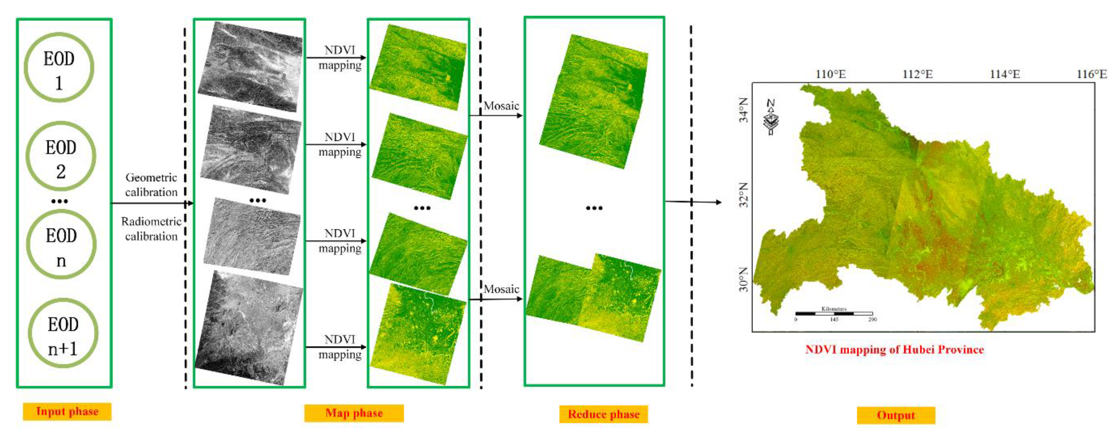
2.2. Kernel Map/Reduce Algorithm for Remote Sensing Imagery Mapping

In the process of remote sensing imagery mapping, imagery processing can be performed in parallel. Similar to the Hadoop map/reduce workflow, the interaction workflow in the Hadoop environment is divided into map and reduce parts. To accomplish the workflow, the standard OGC web service should be introduced. Yue et al. combined the Sensor Observation Service (SOS) [37] and Google Fusion Table to achieve collaborative management of SM and made observations that can be visualized and analyzed on demand via a scalable SOS [38]. The OGC published the Web Processing Service (WPS) in 2007 to define standardized interfaces that facilitate the publishing, discovery, and binding of geospatial processes by clients [39]. Chen et al. proposed a cloud computing-enabled WPS framework for EOD processing [40].

Figure 2 shows the map/reduce workflow for EOD. The workflow displayed in Figure 3 divides the processing procedure for EOD into two sub-processes: mapping and mosaic. Mapping refers to single image mapping based on the SM inversion index. The SM inversion process can be paralleled on several independent machines. However, the single SM inversion results should be mosaicked to generate a complete, large-scale SM mapping result. The general tool employed is the Geospatial Data Abstraction Library (GDAL) [41]. The SM mapping process is completed in the map phase, and the mosaic process is completed in the reduce phase. The SM mapping index can be the Perpendicular Drought Index, Modified Perpendicular Drought Index [42], Normalized Difference Vegetation Index (NDVI), or Green Normalized Difference Vegetation Index [43].

The map/reduce algorithm for EOD mapping is shown in Algorithm 1. The whole algorithm is divided into four steps: configure, map, reduce, and execute. In the algorithm, the execute request triggers the map/reduce implementation to insert the EOD sets. Using the map/reduce application, a new job is created. As shown in Algorithm 1, the job runs the doConfiguration(Path_HDFS, IP_Hadoop, URL_SOS) function to configure the parameters of the job. The map function is implemented by the setMap(EOD_tn, f_SM) function. The reduce function is executed through the setReduce(ST_tn, f_Mosaic) function. The InsertionOutput information is written into the output file through the setOutput(InsertionOutput) function in the reduce phase. The steps in the program are shown in Algorithm 1.

Algorithm 1: Flow of the map/reduce algorithm for mapping EOD

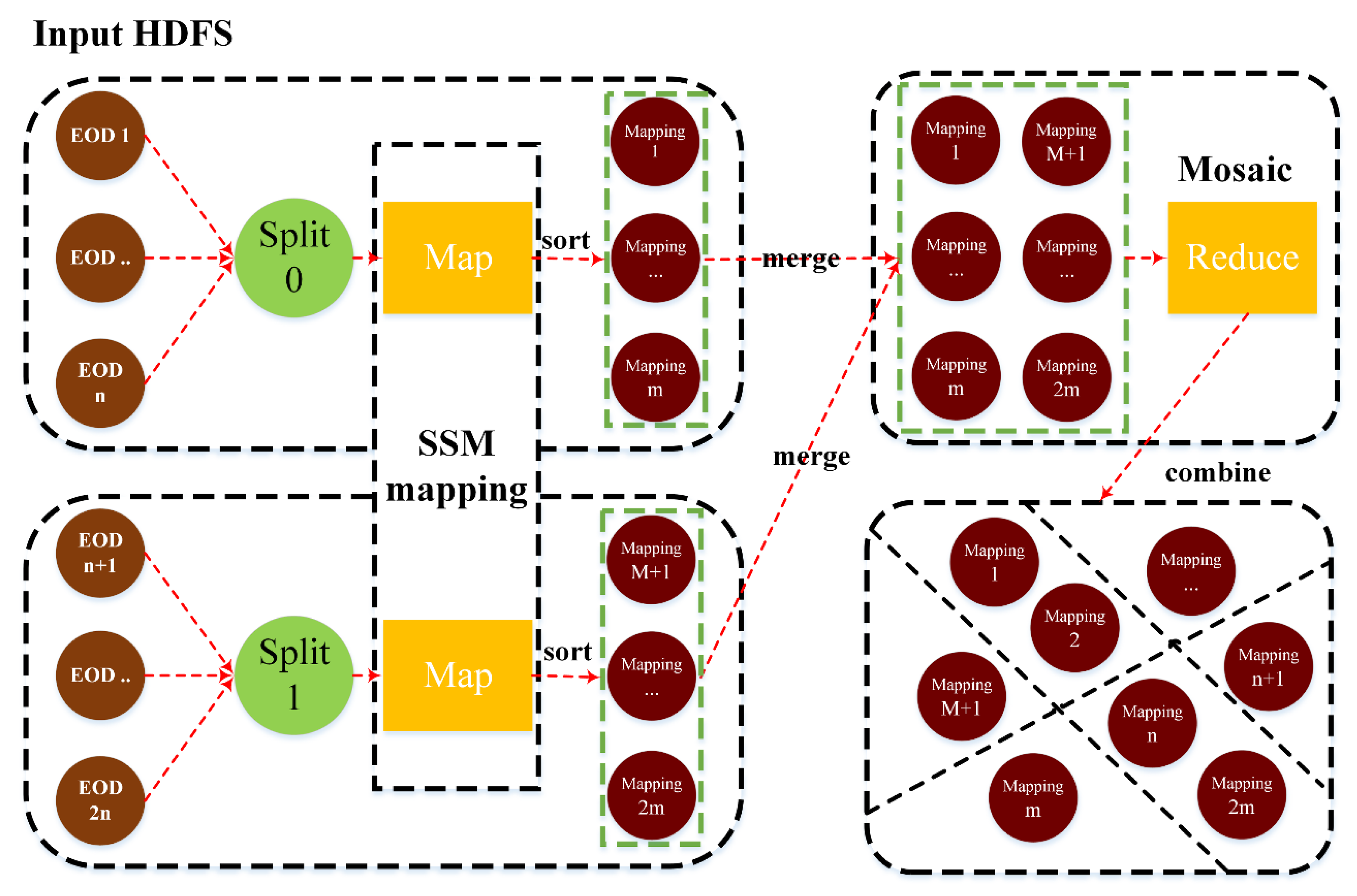
Input: current EOD observation EODtn Output: Insertion result ExecuteOutput indicated by JobStatus Use: WebProcessingService(DatatnInput, AlgorithmIDEOD, ResponseFormat) inherits the data access object for WPS implementation doConfiguration(PathHDFS, IPHadoop, URLSOS) configures PathHDFS and IPHadoop setMap(EODtn, fSM) sets the map function in the map/reduce process setReduce(STtn, fMosaic) sets the distributed database parameters setOutput(InsertionOutput) sets the InsertionOutput status information of the result STEP 1: Inherit the mandatory interface of WPSEOD implementation using the function WebProcessingService(DatatnInput, AlgorithmIDEOD, ResponseFormat), i.e., implement the necessary function embedded in the InsertObservation interface. WPSEOD represents the OGC standard web service that is used to process EOD and generate EOD mapping. STEP 2: Start configuring the parameters of the input path of the Hadoop Distributed File System (HDFS)’s Internet Protocol (IP) address for entry into the Hadoop cluster environment. Create a new job, utilizing the parameters such as IP and port number configured above. HDFS represents the storage layer in the file system. STEP 3: Obtain the set of objects STtn from EODtn using the get4(EODtn) function. The implementation of the get4(EODtn) function is based on the Observation & Measurement encoding model with the help of SOSEOD. SOSEOD represents the OGC standard web service used to access EOD. STEP 4: Implement the map setMap(EODtn, fSM) function, achieving EODtn SM mapping via the fSM function. The decomposition algorithm fSM is called here. After data preprocessing, including geometry correction and radiation correction, EODtn can be mapped via the SM computation model. The specified SM computation model is referenced here. By invoking the application program interface (API) of ArcGIS and the Environment for Visualizing Images (ENVI) tools, SM mapping can be accomplished. ArcGIS and ENVI contain the specific API needed to process the EOD and obtain the SM mapping result. STEP 5: Combine the regional and partial SM maps into a large-scale SM map via the ENVI IDL interface using the setReduce(STtn, fMosaic) function. The fMosaic function refers to the image mosaicking process. The InsertionOutput status information indicated by JobStatus is generated last using the setOutput(InsertionOutput) function. Furthermore, the statistical result will be inserted into the MongoDB database via the SOS data insertion interface and the SOS web address.

2.3. Kernel Map/Reduce Algorithm for in Situ Sensors

In SM monitoring, in situ sensors are diverse and different from each other. These characteristics make them essential for providing seamless observations of SM. As the numbers of sensors and the observation frequency increase, the amount of observation data becomes enormous, making on-the-fly statistical analyses difficult to accomplish. Figure 3 shows the map/reduce workflow for in situ sensors in the proposed framework. The workflow divides the in situ sensors’ observational data sets into two sub-processes: partial-statistic computation and overall-analysis computation. The partial-statistic computation is completed in the map phase, and the overall-analysis computation is completed in the reduce phase in the map/reduce workflow.

In the algorithm, the Execute request triggers the map/reduce implementation to insert the in situ sensors’ observational data sets. Using the map/reduce application, a new job is created. As shown in Algorithm 2, the job runs the doConfiguraion(Path_HDFS, IP_Hadoop, URL_SOS) function to configure the parameters of the job. The map function is implemented by the setMap(In-situObservation_tn, f_{partial-statistic}) function. The reduce function is executed through the setReduce(ST_tn, f_{overall-statistic}) function. The InsertionOutput information is also written into the output file through the setOutput(InsertOutput) function in the reduce phase. To briefly review the principles and components of the Hadoop process, the design of the map/reduce algorithm for an in situ sensor is described in Algorithm 2.

Algorithm 2. Flow of the map/reduce algorithm for an in situ sensor-based statistical analysis

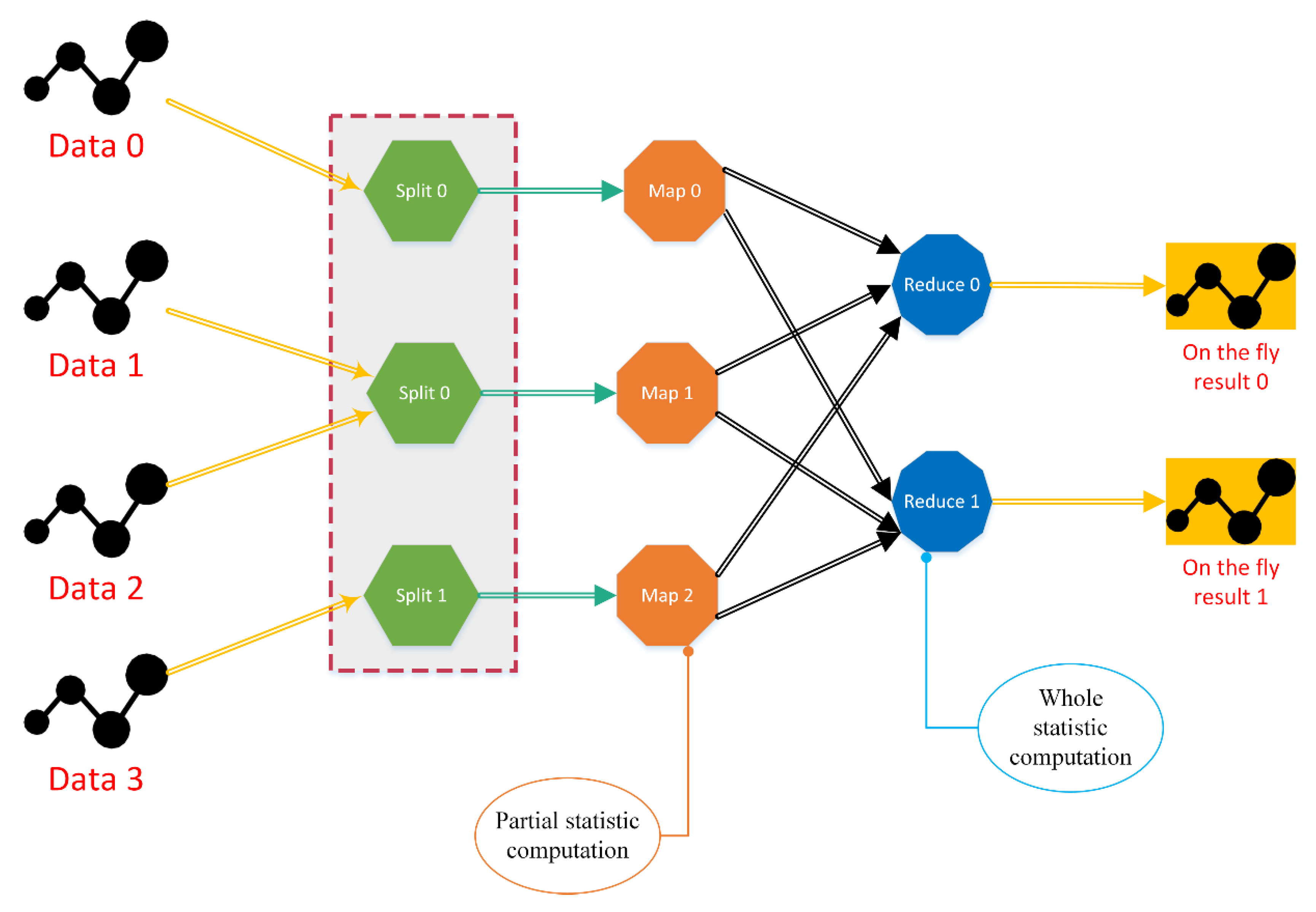
Input: Current in situ sensor observation In-situObservationtn Output: Insertion result ExecuteOutput indicated by JobStatus Use: WebProcessingService(DatatnInput, AlgorithmIDin-situ, ResponseForm) inherits the data access object for WPS implementation doConfiguration(PathHDFS, IPHadoop, URLSOS) configures PathHDFS and IPHadoop setMap(In-situObservationtn, fpartial-statistic) sets the map function in the map/reduce process setReduce(statistictn, foverall-statistic) sets the distributed database parameters setOutput(InsertionOutput) sets the InsertionOutput status information of the result STEP 1: Inherit the mandatory interface of WPSin-situ implementation using the function WebProcessingService(DatatnInput, AlgorithmIDin-situ, ResponseForm), which involves implementing the necessary function embedded in the InsertObservation interface. WPSin-situ represents the OGC standard web service used to process the in situ sensor observations. STEP 2: Start configuring the parameters of the input path of the HDFS’ Internet Protocol address for entry into the Hadoop cluster environment. Create a new job, utilizing parameters such as IP and port number, as configured above. STEP 3: Insert the in situ sensor observation sets into the SOS address automatically via the data insertion interface of the SOS. The observation sets are encoded with the Observation & Measurement encoding model. The in situ sensor observations can be inserted into the MongoDB in this step. The SOS represents the OGC standard web service used to access the in situ sensor observations. STEP 4: Obtain the set of objects STtn from EODtn using the get4(In-situObservationtn) function with the help of SOS. The get4(In-situObservationtn) function is implemented based on the Observation & Measurement encoding model. The spatial and temporal ranges can be specifically set in the following steps. STEP 5: Implement the map function setMap(In-situObservationtn, fpartial-statistic), yielding the In-situObservationtn statistic via the fpartial-statistic function with WPS. The statistic algorithm fpartial-statistic is invoked here to compute the partial statistic result. The statistical algorithm fpartial-statistic is implemented in Java or C#. The partial statistic refers to a partial in situ sensor observational data set statistic. STEP 6: Combine the partial statistic result and the overall statistic result using the function setReduce(statistictn, foverall-statistic). STtn represents the spatiotemporal parameters in foverall-statistic, which is the function used to generate the overall result of all the in situ sensor-based observation sets. The analysis algorithm foverall-statistic is developed in Java or C#. The InsertionOutput status information indicated by JobStatus is generated last with the setOutput(InsertionOutput) function. Overall statistic refers to the overall in situ sensor observational data set statistic.

2.4. Web Service Operation Flow in SM Monitoring

SM management in PA can be divided into two patterns: EOD and in situ sensors. The experimental CESCI server consists of several WPS servers and an SOS server. The WPS servers are implemented from the 52° North WPS, with some improvements, namely, the addition of Hadoop processing for SM computation and an in situ data statistic function. The default database of the 52° North SOS is the PostgreSQL database. Thus, the data observation class should be improved and support the MongoDB.

The web service operation flow is shown in Figure 4. In PA, the deployment of agricultural sensors is critical to obtaining continuous and real-time observations of crops. SM management is designed to achieve on-the-fly statistical analysis of the in situ sensor observations. The SOS can publish data in an open manner using the InsertObservation interface. Therefore, clients on the web can access agricultural data measured in monitored farmland using this SOS. First, the CESCI client delivers the GetCapabilities request to query useable and suitable processes on the server side. The client then obtains the optional and mandatory parameters required by the process through the DescribeProcess interface. The Execute operation is then called to execute this process. Then, JobTracker is triggered to submit the job to the Hadoop NameNode. The job contains the ID, name, process ID, input parameters, and output parameters. By invoking the appropriate algorithm for remote sensors or in situ sensors, the system generates the SM mapping result or the statistical results for in situ sensor observations in the Hadoop environment. In the map/reduce phase, the write process will be repeated at the NameNode and DataNode. The data submitter writes the EOD mapping results or analysis results of the in situ sensor observations to the Hadoop HDFS. The SM mapping and mosaic process is completed in this phase. Then, the result is inserted into the SOS via the data insertion interface. Finally, the entire job is terminated.

3. Experiments

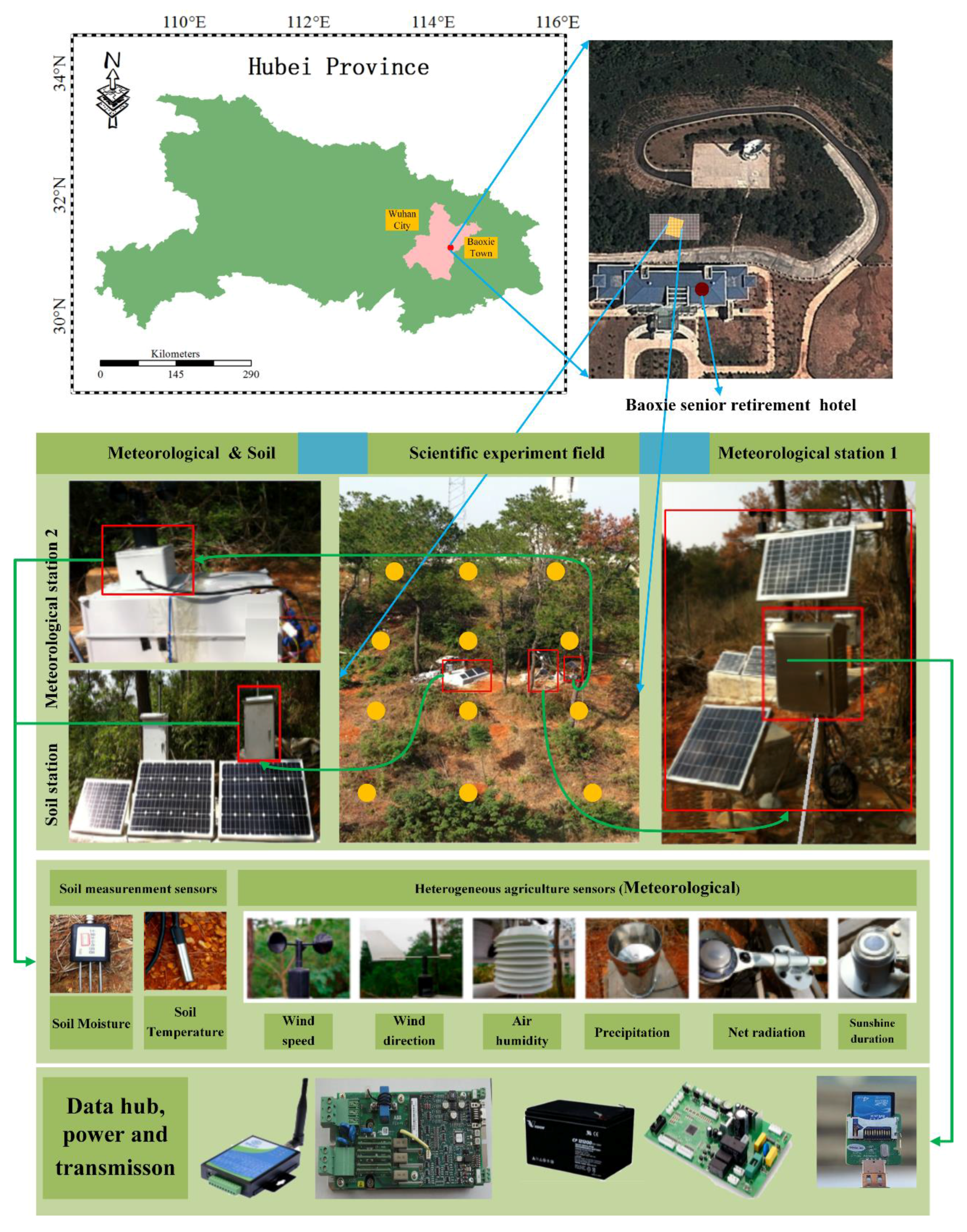
3.1. Experimental Environment

Before the experiment, the distribution environment is established. We employ the Hadoop framework based on the complete distribution method. This framework uses five computers and one switching hub and consists of one name node and four data nodes. The same OS (CentOS 7.0) and Hadoop version 2.6.0 are installed on each node. The configuration of each node is i3 2100 (3.1 GHz), with 8GB RAM. The cluster uses the same hardware as is used in the Hadoop framework. In the Hadoop environment, there are four data nodes and one name node. The Hadoop cluster is deployed on five computers, including one master node and four slave nodes.

3.2. In the Context of Remote Sensing: Earth Observation data Vegetation Index (VI) Mapping

In the context of remote sensing, the chosen study area is Hubei province. GF-1 wide field of view (WFV) 1A imagery is one of the products of the GF-1 satellite, which was recently launched by China in 2013. Handling such large volumes of data from across Hubei province is difficult and time consuming; thus, the proposed CESCI method can be applied here.

Although the VI is not an explicit indicator of SM in most remote sensing cases, VI can generally reveal the SM distribution [44]. As McNally stated, NDVI provides a best guess of soil moisture prediction. NDVI and other remote sensing vegetation indexes can be used to provide early warning for natural hazards such as droughts and floods, which are linked to food insecurity. In the VI mapping experiment, the original data sources are the GF-1 WFV 1A images. To monitor vegetation growth, the VI should be calculated to understand the vegetation. Vegetation in the VI always yields positive values, whereas snow and water yield negative values; thus, VI calculations are important for understanding crop yield [45]. Among the possible VIs, the most widely used VI is the NDVI. Yagci et al. evaluated the effect of crop rotation between corn and soybeans on the accuracy of NDVI-based agricultural drought monitoring in Iowa, USA [46]. Satellite remote sensing has become a popular approach used to analyze agricultural droughts based on terrestrial vegetation health conditions using the NDVI. The NDVI formula is as follows.

$$NDVI=\frac{{\rho }_{NIR}-{\rho }_R}{{\rho }_{NIR}+{\rho }_R}$$

(1)

However, the first formula is utilized in the study. The mosaic process can be the achieved in the reduce step of the map/reduce process. GDAL can be utilized in the mosaic implementation. Different maps covering different spatial areas are combined into one map covering the whole study area. This method can be paralleled with the reduce implementation. Figure 5 shows the MapReduce process used to map the NDVI in Hubei province. First, EODs are geometrically and radiometrically calibrated. Then, the map portion of the map/reduce process is performed. Single preconditioned EOD are used in the NDVI mapping via the application interface (API) ENVI/IDL. In the reduce portion of the map/reduce process, single NDVI maps are mosaicked to achieve a complete NDVI map via the API GDAL. The setMap(), setReduce(), setOutput(), and WebProcessingService() functions are defined as shown in Figure 5. In the setMap() function, the HDFS route, IP, and the NDVI mapping function are set. In the setReduce() function, the mosaic function is set. In the WebProcessingService() function, the NDVI mapping function and mosaic function are implemented.

Through CESCI, the EOD can effectively and efficiently be used for SM mapping. Figure 6 shows the specific performance testing. The time consumption associated with mapping the NDVI using the WPS implementation with a single node based on 128GB and 154GB is 41.2 min and 46.2 min, respectively. The time consumption of CESCI with five nodes is 11.8 min and 13.4 min using 128GB and 154GB, respectively. Hence, the efficiency of CESCI is two times higher than that of the WPS with a single node.

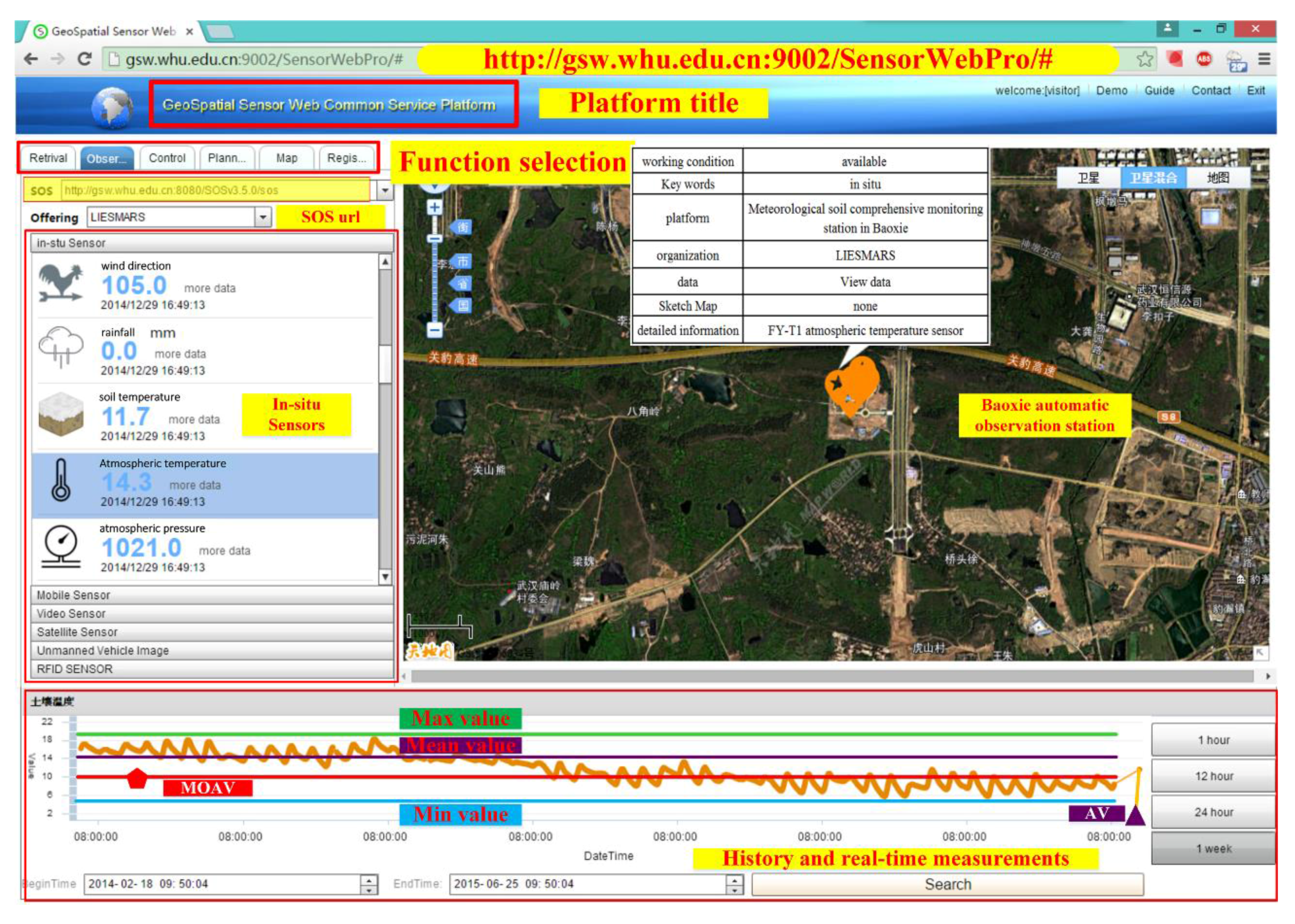
3.3. In the Context of in Situ Sensors: Near Real-Time Analysis

In the context of in situ sensors, the town of Baoxie, which is located in a typical rural area near Wuhan City in Hubei province, China, is selected as a case study. Figure 7 shows the scientific, experimental area, and the date of the experiment is 26 May 2015. Approximately 30 agriculture-related sensors are deployed at an automatic station in a 20 m × 40 m scientific, experimental field (center location at 114°31′35.61”E, 30°28′12.98”N) located in the town of Baoxie, China. SM sensors are deployed in different horizontal planes at three different depths (10 cm, 30 cm, and 40 cm). The meteorological and SM sensors used in this agricultural field are managed and maintained by the Geospatial Sensor Web Common Service Management Platform [47], which allows users to retrieve real-time and historical agriculture-related measurements and map SM in the field.

As Figure 7 shows, the automatic station integrates two meteorological stations and one soil measurement station. SM sensors are used at the soil measurement station. Using GPRS and other hardware devices, the real-time observations are transmitted to the Sensor Web Common Service Management Platform.

In PA, the meteorological sensor observations can be seamless and uninterrupted. However, statistically analyzing the observations in a timely fashion is challenging. Statistical analysis of the geographical data is necessary and meaningful. Improving the timeliness associated with understanding a farm’s evolution and variations, which contain abundant information, is challenging. In summary, the integration of cloud computing technology and PA is possible and essential. By utilizing cloud computing technology, the timeliness of PA analysis will be improved. PA analysis involves extreme value computation, abnormal value selection, and mean value computation. After analyzing the results of this study, we have reached the following conclusions, as listed in

Table 1. Case design of the statistical analysis in the map/reduce process.

Function	Map part (split0 < splitk < splitm, observation[0]~observation[m × n])	Reduce part
Max Value	max[splitk] = observation[splitk × n];	max = max[split0];
	for (i = 1; i++; i < n)	for (i = split1; i++; i < splitm)
	if (observation[splitk × n + i] > max) max[splitk] = observation[splitk × n + i];	if (max[i] > max) max = max[i];
Min Value	min[splitk] = observation[splitk × n];	min = min[split0];
	for (i = 1; i++; i < n)	for (i = split 1; i++; i < splitm)
	if (observation[splitk × n + i] < mix) mix[splitk] = observation[i + splitk × n];	if (min[i] < min) min = min[i];
Mean Value	sum[splitk] = observation[splitk × n];	sum = mean[split0];
	for (i = 1; i++; i < n)	for (i = split1; i++; i < splitm)
	sum[splitk] = sum[splitk] + observation[splitk × n + i];	sum= sum + mean[i];
	mean[splitk] = sum[splitk]/n;	mean = sum/m;
Most Often Appearing Value (MOAV)	MOAV[splitk] = observation[splitk × n];	MOAV = MOAV[split0];
	for (i = 1; i++; i < n)	for (i = split1; i++; i < splitm)
	if (frequency.(observation [splitk × n + i]) > frequency.(MOAV[splitk])) MOAV[splitk] = observation[splitk × n + i];	if (frequency.(MOAV[i]) > frequency.(MOAV)) MOAV = MOAV[i];
Abnormal Value (AV)	AV[splitk] = observation[splitk × n];	None
	for (i = 1; i++; i < n)
	{if (! (Valuemin ≤ observation[splitk × n + i] ≤ Valuemax)) return observation[splitk × n + i];
	continue;
	}

.

The max value is the maximum value in in situ observations, the min value is the minimum value, the mean value is the mean value, and the most often appearing value is the value with the highest rate of occurrence. Changing over time, the value is hard to quantify and determine. Taking value calculation as an example, the map part refers to the max value calculated by circulation in a single data block, and the reduce part refers to the max value calculated by circulation in a max value data block. The map part and reduce part can determine the max value of all in situ observations.

Figure 8 shows the main page of the Geospatial Sensor Web Common Service Platform and the visualization of SM and meteorological observations based on CESCI. The SM curve values are recorded in table form at the bottom of the window. By invoking the SOS interface, the data stored in the SOS will be displayed in the left panel. The left panel shows the SM and meteorological sensors used in the CI. The center of Figure 8 is a map view that displays the geological location of the selected sensor in the left panel. The max values, mean values, min values, most common values, and abnormal values are calculated via the map/reduce algorithm described in Algorithm 1.

Figure 9 shows the observed value, max value, min value, and mean value near real-time curves from 18:44:33 to 20:53:33 on 1 December 2015. The yellow curve is the observed value curve. The purple curve is the mean value. The green curve is the max value. The blue curve is the min value. The max value, min value, mean value, and MOAV can be displayed in near real-time based on the implementation of the algorithm in Section 2.3. SM monitoring can be conducted in near real-time. In PA, near real-time monitoring is essential and indispensable.

Monitoring the SM conditions in the scientific experimental area will enable the detection of the moisture content of the study area. To achieve near real-time SM mapping, the algorithm proposed in Section 2.2 can be applied. The map phase and reduce phase correspond to the statistic and analysis processes. SM in the scientific experimental area can be determined by SM interpolation. The interpolation process can be divided into the map part and reduce part. The SM conditions of blocks can be interpolated based on the SM values at the four surrounding vertices. The map process corresponds to the single interpolation. The reduce part corresponds to the joint interpolation process. Inverse Distance Weighted Interpolation (IDWI), one of the most frequently used spatial interpolation methods, is relatively convenient, commonly used to for computations, and easy to understand [48]. A sampled point’s neighborhood value is calculated via the IDWI model [49]. Figure 10 shows an on-the-fly SM map based on the algorithm in Section 2.2. In this manner, the interpolation is timely. Using the IDWI interpolation method, an SM map can be created to instantly cover the entire experimental area. When choosing the temporal range, the required SM maps are returned to form an SM mapping sequence.

Figure 11 shows the time consumption associated with the interpolation of different numbers of interpolation points in different methods. The time consumption of IDWI WPS implementation with a single node for 1080 and 840 points is 89.2 s and 72.1 s, respectively. The time consumption of CESCI with five nodes is 45.8 s and 35.8 s for 1080 and 840 points, respectively. Hence, the efficiency of CESCI is higher than that of the WPS with a single node. Absolute real-time displays are difficult. However, the interpolation of SM and the calculations of max value, min value, and mean value have been enhanced greatly using CESCI. Thus, in situ sensors and interpolation based on CESCI can effectively reach near real-time.

4. Discussion

4.1. Eligible Algorithm for PA Monitoring Based on Remote Sensing and in Situ Sensors

As almost no attempt has been made to introduce cloud computing into PA, we attempt to create the appropriate combination to propose an eligible monitoring algorithm to effectively monitor the SM condition, as in Section 2.2 and Section 2.3. Implementation has been achieved in Section 3.2 and Section 3.3. In Section 3.2, the time consumption of NDVI mapping has been decreased by CESCI. The in situ sensor observations were analyzed in near real-time in Section 3.3. The max value, min value, mean value, and MOAV can be obtained, and SM interpolation can be achieved in near real-time.

Table 2. Comparisons with other CIs and methods in PA.

CIs and Methods	Characteristic
	SM Mapping Computational Capability	In Situ Observation Analysis Timeliness	Distributed	SOA
CESCI (five nods)	1.4 min/Hubei province	Near real-time	Yes	Yes
Korduan	Unsupported	Unsupported	No	No
Zhang	Unsupported	Near real-time	No	No
Mahmoud	Unsupported	Unsupported	No	No

shows the CESCI comparisons with other CIs and methods. There are two problems in PA monitoring as shown in Table 2: (1) the difficulty associated with supporting EOD processing efficiently to understand the large-scale SM condition due to limited computational capability; and (2) the incapability of performing near real-time analyses of in situ sensor observations in the context of SM conditions. However, the SM mapping computational capability is approximately 1.4 min in Hubei province using the five computational nodes with CESCI. The analysis of in situ observations in near real-time is presented in Section 3.3. The Service-Oriented Architecture (SOA) is the classic architecture applied in CI development. Compared with other CIs and methods, CESCI is SOA enabled. Consequently, PA monitoring with CESCI is effective.

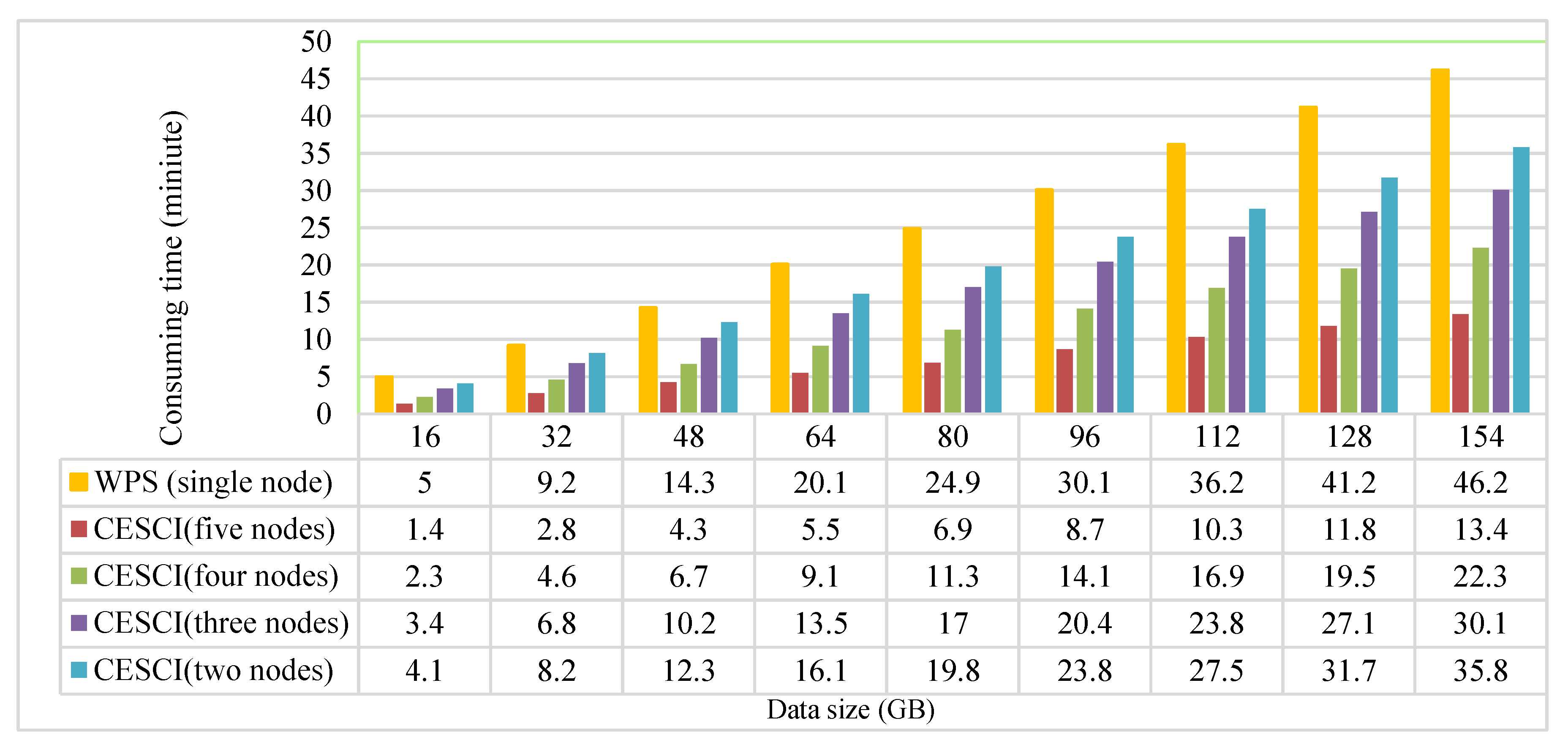
4.2. High-Efficiency Solution for PA Monitoring

The proposed method can be applied to PA monitoring, including enhancing the SM mapping capability and conducting near real-time observation analysis, as performed in the experiments. CESCI addresses the challenge of integrating various interfaces and capabilities by blending remote sensing technology, cyber-physical infrastructure, and high-performance computing technology. For SM mapping, CESCI has achieved performance enhancement, as shown in Section 3.2. With more computational nodes, the performance increases. When dealing with 154GB GF-1 images, the performance of the five-node method is the highest. For in situ sensors, CESCI attempts to achieve near real-time analysis of uninterrupted observations in Section 3.3. The max SM value, min SM value, and mean value calculations can be performed in near real-time, and the interpolation performance of SM mapping at the experimental site was improved with CESCI. Accordingly, PA monitoring with CESCI is an efficient approach.

5. Conclusions and Future Work

Cloud computing plays an important role in PA monitoring platform construction due to its unique advantage associated with data processing, such as in remote sensing image processing and in situ observation interpolation. Therefore, the application of modern technology to improve monitoring performance in PA is essential, as performed in the experiments above. The study proposes the CESCI framework to provide an efficient cyber-physical infrastructure that enables efficient PA monitoring. In the context of remote sensing, the SM mapping performance is enhanced using the map/reduce algorithm. In the context of in situ sensors, the map/reduce algorithm is applied to map sensor-based moisture observations and calculates max/min values and abnormal values in near real-time. In addition, the near real-time SM interpolation was performed with the map/reduce algorithm. With enhanced monitoring capability, the cost of PA monitoring will decrease, and the productivity and income of farmers will increase. In the future, more meaningful functions will be developed to perform deeper data mining and other cloud computing frameworks will be analyzed, such as Spark [31] and Storm [32].

References

1. Zhang, N.; Wang, M.; Wang, N. Precision agriculture—a worldwide overview. Comput. Electron. Agric. 2002, 36, 113–132. [Google Scholar] [CrossRef]
2. Yufeng, G.; Thomasson, J.A.; Sui, R. Remote sensing of soil properties in precision agriculture: A review. Front. Earth Sci. 2011, 5, 229–238. [Google Scholar]
3. Schellberg, J.; Hill, M.J.; Gerhards, R.; Rothmund, M.; Braun, M. Precision agriculture on grassland: Applications, perspectives and constraints. Eur. J. Agron. 2008, 29, 59–71. [Google Scholar] [CrossRef]
4. Sidorova, V.A.; Zhukovskii, E.E.; Lekomtsev, P.V.; Yakushev, V.V. Geostatistical analysis of the soil and crop parameters in a field experiment on precision agriculture. Eurasian Soil Sci. 2012, 45, 783–792. [Google Scholar] [CrossRef]
5. Silva, C.B.; Moraes, M.A.F.D.D.; Molin, J.P. Adoption and use of precision agriculture technologies in the sugarcane industry of Sao Paulo state, Brazil. Precis. Agric. 2011, 12, 67–81. [Google Scholar] [CrossRef]
6. Brocca, L.; Melone, F.; Moramarco, T.; Morbidelli, R. Soil moisture temporal stability over experimental areas in Central Italy. Geoderma 2009, 148, 364–374. [Google Scholar] [CrossRef]
7. Legates, D.R.; Mahmood, R.; Levia, D.F.; DeLiberty, T.L.; Quiring, S.M.; Houser, C.; Nelson, F.E. Soil moisture: A central and unifying theme in Physical Geography. Prog. Phys. Geog. 2011, 35, 65–86. [Google Scholar] [CrossRef]
8. Cho, E.; Choi, M.; Wagner, W. An assessment of remotely sensed surface and root zone soil moisture through active and passive sensors in northeast Asia. Remote Sens. Environ. 2015, 160, 166–179. [Google Scholar] [CrossRef]
9. Entekhabi, D.; Rodriguez-Iturbe, I.; Castelli, F. Mutual interaction of soil moisture state and atmospheric processes. J. Hydrol. 1996, 184, 3–17. [Google Scholar] [CrossRef]
10. Finn, M.P.; Lewis, M.D.; Bosch, D.D.; Giraldo, M.; Yamamoto, K.; Sullivan, D.G.; Kincaid, R.; Luna, R.; Allam, G.K.; Kvien, C.; et al. Remote Sensing of Soil Moisture Using Airborne Hyperspectral Data. GISci. Remote Sens. 2011, 48, 522–540. [Google Scholar] [CrossRef]
11. Aquino-Santos, R.; González-Potes, A.; Edwards-Block, A.; Virgen-Ortiz, R.A. Developing a new wireless sensor network platform and its application in precision agriculture. Sensors 2011, 11, 1192–1211. [Google Scholar] [CrossRef] [PubMed]
12. Srbinovska, M.; Gavrovski, C.; Borozan, V.; Dimcev, V.; Krkoleva, A. Environmental parameters monitoring in precision agriculture using wireless sensor networks. J. Clean. Prod. 2015, 88, 297–307. [Google Scholar] [CrossRef]
13. Lausch, A.; Zacharias, S.; Dierke, C.; Pause, M.; Kühn, I.; Doktor, D. Analysis of vegetation and Soil Patterns using Hyperspectral Remote Sensing, EMI, and Gamma-Ray Measurements. Vadose Zone J. 2013, 12, 108–112. [Google Scholar] [CrossRef]
14. Gooley, L.; Huang, J.; Pagé, D.; Triantafilis, J. Digital soil mapping of available water content using proximal and remotely sensed data. Soil Use Manag. 2013, 30, 139–151. [Google Scholar] [CrossRef]
15. Hao, C.; Zhang, J.; Yao, F. Combination of multi-sensor remote sensing data for drought monitoring over Southwest China. Int. J. Appl. Earth Obs. 2015, 35, 270–283. [Google Scholar] [CrossRef]
16. Botts, M.; Percivall, G.; Reed, C.; Davidson, J. OGC Sensor Web Enablement: Overview and High Level Architecture; Open Geospatial Consortium: Wayland, MA, USA, 2008. [Google Scholar]
17. Bröring, A.; Echterhoff, J.; Jirka, S.; Simonis, I.; Everding, T.; Stasch, C.; Liang, S.; Lemmens, R. New generation sensor web enablement. Sensors 2011, 11, 2652–2699. [Google Scholar] [CrossRef] [PubMed]
18. Stewart, C.A.; Simms, S.; Plale, B.; Link, M.; Hancock, D.Y.; Fox, G.C. What is cyberinfrastructure? In Proceedings of the 38th annual ACM SIGUCCS fall conference: Navigation and discovery, Norfolk, VI, USA, 24–27 October 2010.
19. Moghaddam, M.; Entekhabi, D.; Goykhman, Y.; Li, K.; Liu, M.; Mahajan, A.; Nayyar, A.; Shuman, D.; Teneketzis, D. A wireless soil moisture smart sensor web using physics-based optimal control: Concept and initial demonstrations. IEEE J. Sel. Top. Appl. Earth Obs. Remote Sens. 2010, 3, 522–535. [Google Scholar] [CrossRef]
20. Cyberinfrastructure Software Sustainability and Reusability: Report from an NSF-funded Workshop. Available online: https://scholarworks.iu.edu/dspace/handle/2022/6701 (accessed on 27 May 2016).
21. Wang, S.; Zhu, X.G. Coupling cyberinfrastructure and geographic information systems to empower ecological and environmental research. BioScience 2008, 58, 94–95. [Google Scholar] [CrossRef]
22. Wright, D.J.; Wang, S. The emergence of spatial cyberinfrastructure. Proc. Natl. Acad. Sci. USA 2011, 108, 5488–5491. [Google Scholar] [CrossRef] [PubMed] [Green Version]
23. Wang, S.; Liu, Y. TeraGrid GIScience gateway: Bridging cyberinfrastructure and GIScience. Int. J. Geogr. Inf. Sci. 2009, 23, 631–656. [Google Scholar] [CrossRef]
24. Wang, S.; Anselin, L.; Bhaduri, B.; Crosby, C.; Goodchild, M.F.; Liu, Y.; Nyerges, T.L. CyberGIS software: A synthetic review and integration roadmap. Int. J. Geogr. Inf. Sci. 2013, 27, 2122–2145. [Google Scholar] [CrossRef]
25. Phillips, A.J.L.; Newlands, N.K.; Liang, S.H.L.; Ellert, B.H. Integrated sensing of soil moisture at the field-scale: sampling, modelling and sharing for improved agricultural decision-support. Comput. Electron. Agric. 2014, 107, 73–88. [Google Scholar] [CrossRef]
26. Korduan, P.; Bill, R.; Böling, S. An interoperable Geodata infrastructure for precision agriculture. In Proceedings of the 7th AGILE Conference on Geographic Information Science, Heraklion, Greece, 29 April–1 May 2004.
27. Zhang, X.; Seelan, S.; Seielstad, G. Digital northern great plains: A web-based system delivering near real time remote sensing data for precision agriculture. Remote Sens. 2010, 2, 861–873. [Google Scholar] [CrossRef]
28. Abdelfattah, M.A.; Kumar, A.T. A web-based GIS enabled soil information system for the United Arab Emirates and its applicability in agricultural land use planning. Arab. J. Geosci. 2014, 8, 1–15. [Google Scholar] [CrossRef]
29. Stanoevska-Slabeva, K.; Wozniak, T.; Ristol, S. (Eds.) Grid and Cloud Computing: A Business Perspective on Technology and Applications; Springer: Berlin, Germany, 2010.
30. Chung, W.C.; Chen, C.C.; Jm, H.; Lin, C.Y.; Hsu, W.L.; Wang, Y.C.; Lee, D.T.; Lai, F.; Huang, C.W.; Chang, Y.J. CloudDOE: A user-friendly tool for deploying Hadoop clouds and analyzing high-throughput sequencing data with MapReduce. PLoS ONE 2014, 9, e98146. [Google Scholar] [CrossRef] [PubMed]
31. Chen, C.L.P.; Zhang, C.Y. Data-intensive applications, challenges, techniques and technologies: A survey on big data. Inform. Sci. 2014, 275, 314–347. [Google Scholar] [CrossRef]
32. Yang, W.; Liu, X.; Zhang, L.; Yang, L.T. Big data real-time processing based on storm. In Proceedings of the 12th IEEE International Conference on Trust, Security and Privacy in Computing and Communications, Melbourne, VIC, Australia, 16–18 July 2013; Volume 8, pp. 1784–1787.
33. Dean, J.; Ghemawat, S. MapReduce: Simplified data processing on large clusters. Commun. ACM 2008, 51, 107–113. [Google Scholar] [CrossRef]
34. Juve, G.; Deelman, E.; Berriman, G.B.; Berman, B.P.; Maechling, P. An evaluation of the cost and performance of scientific workflows on Amazon EC2. J. Grid Comput. 2012, 10, 5–21. [Google Scholar] [CrossRef]
35. Behzad, B.; Padmanabhan, A.; Liu, Y.; Liu, Y.; Wang, S. Integrating CyberGIS gateway with Windows Azure: A case study on MODFLOW groundwater simulation. In Proceedings of the ACM SIGSPATIAL Second International Workshop on High Performance and Distributed Geographic Information Systems, Chicago, IL, USA, 1 November 2011; pp. 26–29.
36. Jiang, W.; Zhang, L.; Liao, X.; Jin, H.; Peng, Y. A novel clustered MongoDB-based storage system for unstructured data with high availability. Computing 2014, 96, 455–478. [Google Scholar] [CrossRef]
37. Bröring, A.; Stasch, C.; Echterhoff, J. OGC Sensor Observation Service Interface Standard; Version 2.0; Open Geospatial Consortium: Wayland, MA, USA, 2012. [Google Scholar]
38. Yue, P.; Jiang, L.; Hu, L. Google fusion tables for managing soil moisture sensor observations. IEEE J. Sel. Top. Appl. Earth Obs. Remote Sens. 2014, 7, 4414–4421. [Google Scholar] [CrossRef]
39. Schut, P. OpenGIS Web Processing Service; Open Geospatial Consortium: Wayland, MA, USA, 2007. [Google Scholar]
40. Chen, Z.; Chen, N.; Yang, C.; Di, L. Cloud computing enabled web processing service for earth observation data processing. IEEE J. Sel. Top. Appl. Earth Obs. Remote Sens. 2012, 5, 1637–1649. [Google Scholar] [CrossRef]
41. Qin, C.; Zhan, L.; Zhu, A. How to apply the Geospatial Data Abstraction Library (GDAL) properly to parallel geospatial raster I/O? Trans. GIS 2014, 18, 950–957. [Google Scholar] [CrossRef]
42. Ghulam, A.; Qin, Q.; Teyip, T.; Li, Z. Modified Perpendicular Drought Index (MPDI): A real-time drought monitoring method. ISPRS J. Photogramm. Remote Sens. 2007, 62, 150–164. [Google Scholar] [CrossRef]
43. Candiago, S.; Remondino, F.; de Giglio, M.; Dubbini, M.; Gattelli, M. Evaluating multispectral images and vegetation indices for precision farming applications from UAV images. Remote Sens. 2015, 7, 4026–4047. [Google Scholar] [CrossRef]
44. McNally, A.; Shukla, S.; Arsenault, K.R.; Wang, S.; Peters-Lidard, C.D.; Verdin, J.P. Evaluating ESA CCI soil moisture in east Africa. Int. J. Appl. Earth Obs. 2016, 48, 96–109. [Google Scholar] [CrossRef]
45. Xiao, Z.; Liang, S.; Wang, T.; Liu, Q. Reconstruction of satellite-retrieved land-surface reflectance based on temporally-continuous vegetation indices. Remote Sens. 2015, 7, 9844–9864. [Google Scholar] [CrossRef]
46. Yagci, A.L. The effect of corn–soybean rotation on the NDVI-based drought indicators: A case study in Iowa, USA, using vegetation condition index. Gisci. Remote Sens. 2015, 52, 290–314. [Google Scholar] [CrossRef]
47. Geospatial Sensor Web Common Service Management Platform. Available online: http://gsw.whu.edu.cn:9002/SensorWebPro/# (accessed on 22 October 2015).
48. Lu, G.; Wong, D. An adaptive inverse-distance weighting spatial interpolation technique. Comput. Geosci. 2008, 34, 1044–1055. [Google Scholar] [CrossRef]
49. Mueller, T.G.; Pusuluri, N.B.; Mathias, K.K.; Cornelius, P.L.; Barnhisel, R.I.; Shearer, S.A. Map quality for ordinary kriging and inverse distance weighted interpolation. Soil Sci. Soc. Am. J. 2004, 68, 2042–2047. [Google Scholar] [CrossRef]
Figure 1. Architecture of the cloud computing-enabled spatio-temporal cyber-physical information infrastructure.
Ijgi 05 00081 g001
Figure 2. Map/reduce workflow for EOD in the proposed Framework. EODx represents the specific remote sensing image, such as a GF-1 image, and mappingx represents the SM mappingx inverted by the SM inversion index.
Ijgi 05 00081 g002
Figure 3. Map/reduce workflow of in situ sensors in the proposed framework.
Ijgi 05 00081 g003
Figure 4. Web service operation flow in SM monitoring.
Ijgi 05 00081 g004
Figure 5. The MapReduce process used to map the NDVI in Hubei province.
Ijgi 05 00081 g005
Figure 6. Time consumption associated with mapping the NDVI in Hubei province using the WPS (single node), CESCI (five nodes), CESCI (four nodes), CESCI (three nodes), and CESCI (two nodes) methods.
Ijgi 05 00081 g006
Figure 7. Experimental site and the entire monitoring system of deployed sensors.
Ijgi 05 00081 g007
Figure 8. The Geospatial Sensor Web Common Service Platform and the visualization of SM and meteorological observations based on the proposed CESCI.
Ijgi 05 00081 g008
Figure 9. The SM value, max SM value, min SM value, and mean SM value near real-time curves.
Ijgi 05 00081 g009
Figure 10. The Web portal, showing an on-the-fly SM map based on the proposed cyber-physical infrastructure.
Ijgi 05 00081 g010
Figure 11. Time consumption of interpolation of different numbers of interpolation points using the WPS (single node), CESCI (five nodes), CESCI (four nodes), CESCI (three nodes), and CESCI (two nodes) methods.
Ijgi 05 00081 g011