OpenCL Implementation of a Parallel Universal Kriging Algorithm for Massive Spatial Data Interpolation on Heterogeneous Systems

Abstract

In some digital Earth engineering applications, spatial interpolation algorithms are required to process and analyze large amounts of data. Due to its powerful computing capacity, heterogeneous computing has been used in many applications for data processing in various fields. In this study, we explore the design and implementation of a parallel universal kriging spatial interpolation algorithm using the OpenCL programming model on heterogeneous computing platforms for massive Geo-spatial data processing. This study focuses primarily on transforming the hotspots in serial algorithms, i.e., the universal kriging interpolation function, into the corresponding kernel function in OpenCL. We also employ parallelization and optimization techniques in our implementation to improve the code performance. Finally, based on the results of experiments performed on two different high performance heterogeneous platforms, i.e., an NVIDIA graphics processing unit system and an Intel Xeon Phi system (MIC), we show that the parallel universal kriging algorithm can achieve the highest speedup of up to 40× with a single computing device and the highest speedup of up to 80× with multiple devices.

1. Introduction

Spatial Interpolation (SI) is a process employed to estimate the values of properties at unknown points within an area covered by existing observed points [1]. In many situations, SI is performed to provide contours so data can be displayed graphically, to calculate property values for the surface at a given point or to analyze and predict a trend surface. In Digital Earth (DE) research, SI has always been a powerful tool for modeling and simulation [2,3]. Technological developments have greatly enriched the methods that are available for acquiring and accessing data, and in many large-scale engineering applications, huge amounts of data need to be processed using interpolation algorithms. Indeed, SI is particularly important for prediction and representation in many fields, including geographical information systems and remote sensing [4,5,6], geology [7], mining [8], hydrogeology [9], soil research [10], geophysics [11], oceanography [12], meteorology [13], ecology and environmental studies [14,15].

Several different types of classification methods are used by SI procedures, e.g., point-area, global-local and exact-approximate interpolation [16]. Many techniques exist for both global and local interpolation. Trend surface analysis and Fourier series are examples of global techniques, whereas proximal, kriging and B-splines are local techniques. In particular, the kriging SI algorithm is a typical local interpolation algorithm. The universal kriging interpolation algorithm is a type of linear and unbiased optimal kriging SI algorithm, which is used widely in many scientific and engineering applications. However, in many applications, severe performance bottlenecks occur when using the serial universal kriging algorithm because the computational cost increases exponentially with the input data size [17,18].

In order to accelerate the process and obtain better performance, researchers have developed different methods in the past decades to implement parallel SI algorithms that target high performance computing systems, e.g., MasPar [19], Cray T3D [20], parallel clusters [21], multi-core platforms [22] and grid computing environments [23]. In particular, there have been several studies of parallel kriging interpolation algorithm design. For example, Kerry et al. [24] used a dedicated high performance computer to implement a parallel kriging algorithm that greatly reduces the CPU time. However, this method is quite expensive, and it demands a high standard hardware configuration to accelerate processing. Pedelty et al. [25] implemented a parallel kriging algorithm using the message passing interface parallel programming model on a commodity cluster, where their implementation achieved satisfactory performance and good efficiency. However, the requirement for real-time processing and the rapid growth in the data size demands many more computing nodes, which inevitably increases both the hardware and maintenance costs, as well as requiring high energy consumption [26]. Some studies have also developed parallel kriging algorithms using multi-core parallelism methods. For example, Strzelczyk et al. [27] designed a parallel kriging algorithm based on multiple cores, but there were efficiency issues when multi-core parallelism was applied to specialized scientific applications, e.g., big data processing, because of the slow system memory access.

Recently, due to the rapid increase in the computing capacity of accelerators, such as Graphics Processor Units (GPUs) and Intel Xeon Phi (Intel Many Integrated Core architecture (MIC)), the use of accelerators for big data processing has become a hot research topic in various fields. Many studies of GPUs have been conducted in the geo-sciences field [28,29,30,31]. In particular, there have been some studies of universal kriging algorithms; for example, Cheng et al. implemented a parallel universal kriging algorithm using the NVIDIA Compute Unified Device Architecture (CUDA) on a GPU platform [32]. However, there have been few studies on the Intel MIC platform because MIC is a relatively new accelerator technology. Previous studies based on MIC focused mainly on comparisons with GPU or programming aspects of the platform instead of the design or implementation of a parallel SI algorithm or applications. For instance, Heinecke et al. [33] compared the architecture and performance of a General Purpose GPU (GPGPU) with an Intel MIC and demonstrated the benefits of MIC. Wang et al. [34] described measures to avoid bottlenecks in the memory capacity, network bandwidth, etc., and enhanced the parallel programming thread extensibility on the MIC platform. However, their implementations were not portable across different platforms because different computing platforms, i.e., GPU and MIC, require different programming models and tools.

A heterogeneous computing system is a computing system that can integrate the GPU and Intel Xeon Phi acceleration components into conventional computing systems to implement computing tasks together with the CPU. Heterogeneous computing integrates each heterogeneous platform in an asynchronous manner by utilizing separate resources for computing or task scheduling, thereby maximizing the overall efficiency of a computing system by assigning tasks based on considerations of the capacities of each computing device [35].

Heterogeneous computing is playing increasingly important roles in big data processing, and we envision the rapid adoption of heterogeneous computing for large-scale spatial data interpolation processing using improved algorithms. This approach can potentially achieve high performance on coprocessor computing platforms with speedups of more than 10×, as well as effectively avoiding the aforementioned problems that are encountered on a traditional CPU-only cluster. It is also desirable to have an optimized cross-platform implementation of a parallel universal kriging algorithm that runs on different heterogeneous platforms. To the best of our knowledge, few studies have addressed the application of heterogeneous computing in the geo-sciences field.

In this study, we present the design and implementation of a parallel universal kriging algorithm, as well as demonstrating its performance and cross-platform features. The remainder of this paper is organized as follows. In Section 2, we give a brief introduction to the universal kriging algorithm, heterogeneous computing and the OpenCL development model. Section 3 focuses on the implementation of the serial kriging algorithm, hotspot analysis and the corresponding parallelization techniques. In Section 4, we describe the design and implementation of the parallel universal kriging algorithm. Section 5 presents the experimental results and analysis. Finally, we give our conclusions in Section 6.

2. Background

2.1. Principle of the Universal Kriging Interpolation Algorithm

The universal kriging algorithm is a type of linear unbiased optimal SI algorithm. In contrast to other commonly-used SI algorithms, such as Voronoi and the inverse distance weighting method [36], it considers the spatial correlation between the points that need to be interpolated and their neighboring points, as well as giving the estimation error. The universal kriging algorithm provides more accurate interpolation results, and it is applied widely in the geological interpolation area. The principle of the algorithm is expressed by Equation (1):

$$Z^{*}\left(x_0\right)={\displaystyle \sum }_{i=1}^n{\lambda }_{i}Z\left(x_i\right)$$

(1)

where $Z^{*}\left(x_0\right)$ is the value at the point that needs to be interpolated and ${\lambda }_i$ represents the weighted coefficient of point $i$, with the measured value $Z\left(x_i\right)$. When the expectation of random variable $Z\left(x\right)$ is a variable in the area of interest, we have,

$$E\left[Z\left(x\right)\right]=m\left(x\right)$$

(2)

In this case, the universal kriging algorithm is required for interpolation. In Equation (2), $m\left(x\right)$ is the drift function, which can be represented as follows,

$$m\left(x\right)={\displaystyle \sum }_{l=0}^k{u}_l{f}_l\left(x\right)$$

(3)

where $f_l\left(x\right)$ is a known equation and $u_l$ is the unknown parameter. To ensure that the evaluated and estimated values are as similar as possible, the universal kriging interpolation algorithm should meet the following two conditions.

• Condition 1: The unbiased condition, i.e., the expected value of the difference between the evaluated and estimated values is zero, $E\left[Z^{*}\left(x_0\right)-Z\left(x_0\right)\right]\equiv 0$, which leads to the equation: ${{\displaystyle \sum }}_{i=1}^n{\lambda }_i=1$. By combining this with Equations (1) and (3), the universal kriging algorithm can be expressed by Equation (4).

  $${\displaystyle \sum }_{i=1}^n{\lambda }_i{f}_l\left(x_i\right)=f_l\left(x_0\right), \left(l=0, 1,\dots ,k\right)$$

  (4)
• Condition 2: The estimated minimum variance conditions. To minimize the variance between the estimated and measured value, the universal kriging interpolation algorithm needs to satisfy the following condition.

  $${\sigma }_E^2=E{\left[Z^{*}\left(x_0\right)-Z\left(x_0\right)\right]}^2$$

  (5)

Using Equations (1) and (5), we can obtain Equation (6).

$${\sigma }_E^2=-{\displaystyle \sum }_{i=1}^n{\displaystyle \sum }_{j=1}^n{\lambda }_i{\lambda }_j\gamma (x_i,x_j)+2{\displaystyle \sum }_{i=1}^n{\lambda }_i\gamma \left(x_i, x_0\right)$$

(6)

where $\gamma$ means the variation function. Using the Lagrange multiplier method and Equations (4) and (6), we can obtain the target function, as shown in Equation (7).

$$F={\sigma }_E^2-2{\displaystyle \sum }_{l=0}^k{u}_l\left[{\displaystyle \sum }_{i=1}^n{\lambda }_i{f}_l\left(x_i\right)-f_l\left(x_0\right)\right]$$

(7)

By taking the partial derivatives of ${\lambda }_i$ and $u_l$, and making them equal to zero, we obtain the equation set of the universal kriging algorithm. The estimated values of the points of interest are obtained by solving the corresponding equations in matrix form, which comprises a series of product operations for the measured value and the corresponding weight of each point.

2.2. Heterogeneous Computing

A heterogeneous computing system comprises different processors with diverse functions or performance, which connect via a specific interconnection structure. In general, they comprise one or more general purpose microprocessors and special accelerated processors. At present, the most widely-used heterogeneous computing platforms contain both CPU and GPU. NVIDIA released the first general purpose GPU in 1999, which was a dedicated coprocessor designed to solve the problem of complex calculations [37]. Due to its highly parallel multi-core structure and higher memory access bandwidth, the GPU offers higher peak computing capacities and higher memory throughput than the contemporary CPU. With support from CUDA and OpenCL, it has gradually become a type of general-purpose processor. On 18 June 2012, Intel Cooperation introduced the MIC (Many Integrated Core architecture) platform, which is a many-core architecture that differs from that of a GPU [38]. MIC is a coprocessor with a multiple ×86 core architecture. These cores are integrated into a single computing node as coprocessor hardware peripherals, and they work together with the CPU. MIC is compatible with the ×86 CPU instruction set and the single instruction-multiple data instruction sets, which can reduce the difficulty of transplantation from a traditional cluster to the MIC architecture. In addition, it supports complex, but flexible programming strategies. Thus, MIC has led application development into a new period. The combination of CPU and MIC provides a new option for heterogeneous computing.

The experiments presented in this study were performed on two heterogeneous computing platforms: a CPU + GPU platform called Shelob located at Louisiana State University in the United States and a CPU + MIC platform at Tsinghua University in China.

2.3. OpenCL Programming Model

OpenCL is the first general parallel programming standard for heterogeneous computing. It was originally developed by Apple Incorporated, and it is free, cross-platform, with good interoperability [39]. OpenCL provides a unified programming environment for software developers. It facilitates the development of software for high performance computing servers, desktop computing systems and hand-held devices, as well as applications in multicore processors (CPU/MIC), GPUs, digital signal processors and other many-core processors. OpenCL has many application fields, and it has a promising future in the consumer market.

OpenCL is an implementation rather than a developing language. It provides the C-like programming language (based on C99) to develop a kernel function that can run on different OpenCL devices and a group of application programming interfaces (APIs), which can define and control heterogeneous platforms. OpenCL provides two parallel computing mechanisms [35], i.e.: (1) based on task segmentation; and (2) based on data segmentation. According to the official manual for OpenCL development, the constructed algorithms/applications can run on a variety of equipment. Furthermore, OpenCL supports the implementation of multiple levels of parallelism, and each parallelism level can be mapped efficiently onto hardware on homogeneous or heterogeneous architectures. During the design and development of a parallel algorithm that is compliant with the OpenCL specification, it is important to follow four prescribed models, i.e., the platform model, the implementation model, the memory model and the programming model. The platform model is a high-level description of the heterogeneous computing system with abstractions to the system’s hardware basis. The implementation model describes how the kernels run on the OpenCL platform and how the kernel interacts with the host end. The memory model is an abstraction of the underlying memory space, which describes the memory area set in OpenCL and defines the interactions of different memory spaces during calculations. The programming model is a high-level abstraction of the applications implemented by program developers, which defines the mappings of the OpenCL program with the host and the processing unit with the memory spaces.

A parallel algorithm will achieve better performance if suitable memory types are considered during OpenCL programming. OpenCL defines a four-level memory hierarchy for the computing device: global, constant, local and private memory. The global memory can be shared by all of the processing elements, but it has high access latency. The constant memory is also visible to all of the computing units on the device, where it is part of the global memory. Any element of the constant memory is accessible simultaneously to all of the work-items. The local memory belongs to the computing unit and it is typically implemented on-chip, where it is shared by all of the work-items within a workgroup. It has low access latency, but its capacity is limited. Private memory belongs to a work-item, and it is typically implemented on-chip in registers.

OpenCL has gained wide support from major coprocessor manufacturers, and it has the advantages of being open source and cross-platform [39], so in this study, we used OpenCL as our development tool to implement the parallel universal kriging algorithm on different heterogeneous computing platforms.

3. Serial Universal Kriging Algorithm

3.1. Implementation of the Serial Universal Kriging Algorithm

The primary task involved in the implementation of the serial algorithm is selecting an appropriate space variation function model, as well as code development for this variation function model. In this study, we calculate the estimated value for each point using the neighboring points searching approach.

3.1.1. Selecting the Variation Function Model

The variation function model can be divided into three categories in geo-statistics: (1) the model with sill [40], which includes a spherical model, an index model and a Gaussian model; (2) the model without sill [2], which includes a power function and a linear model; and (3) the cavity effect model [41]. We use the spherical model, which is employed frequently in geo-statistics, as our serial universal kriging algorithm’s variogram function. The spherical model can be expressed by Equation (8):

$$\gamma \left(h\right)=\{\begin{array}{cc}0& h=0\hfill \\ c_0+c\left(\frac{3h}{2a}-\frac{h^3}{2a^3}\right)& 0<h\le a\hfill \\ c_0+c& h>a\hfill \end{array}$$

(8)

where $c_0$ is the nugget effect, c is the partial sill of the semi-variogram model and a is the range of influence.

3.1.2. Implementation of the Serial Algorithm

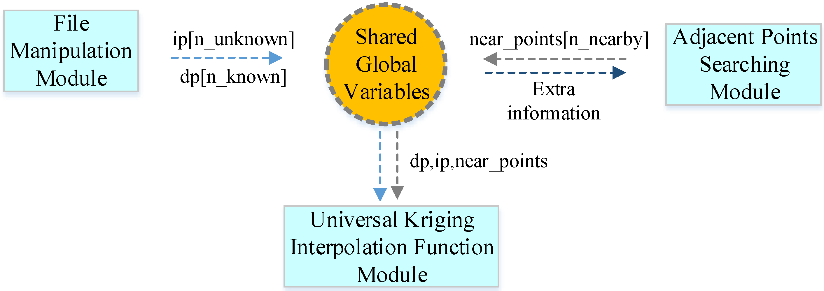
Following the principle of the universal kriging algorithm, using the selected variation function, the serial algorithm can be implemented based mainly on three components: (1) the File Manipulation Module (FMM); (2) the Adjacent Points Searching Module (APSM); and (3) the Universal Kriging Interpolation Function Module (UKIFM). FMM is responsible for reading the input shape file to obtain the three-dimensional coordinates for the known points and other information. When the interpolation results are ready, this module also writes the data as the output. These functions are implemented using an open-source spatial data format conversion library, GDAL (Geospatial Data Abstraction Library) [16]. APSM focuses mainly on calculating the plane coordinates $\left(x, y\right)$ of the unknown points according to the coordinate range of the known points and using a fixed step. The n neighbor points of every unknown point are searched where the searching procedure employs the k-nearest neighborhood algorithm [42], which searches k neighbors of the search point. The UKIFM module is the numerical kernel used for interpolation (see Figure 1).

All of the modules use some shared global variables to complete data interaction and data processing. First, the serial algorithm needs two global arrays, i.e., double dp[n_known] and ip[n_unknown] in FMM, where the former is for the known points and the latter is for the points where interpolation takes place. Thus, the array dp[n_known] is initialized to store the data extracted from the input shape file, and the array ip[n_unknown] is filled with the plane coordinates’ information, i.e., $\left(x, y\right)$, for each unknown point by searching the appropriate points with a fixed step length on a global scale for the whole input image. Second, during the search process, an extra array called double near_points[n_nearby] is introduced to store the n_nearby adjacent points found for each unknown point. Third, UKIFM uses the plane coordinates $\left(x, y\right)$ of the unknown points and the coordinates of their corresponding adjacent points to calculate the estimated values, which are output together with the coordinates, i.e., $\left(x, y, z\right)$ for these unknown points.

Specifically, the serial algorithm can be expressed in detail by the following four steps.

• Step (1): Read the data information, i.e., $\left(x, y, z\right)$, the three-dimensional coordinates of the known points from source files.
• Step (2): Calculate the plane coordinates of the unknown points according to the coordinate range of the known points. Based on the known points, select the points that need to be interpolated with a specified space interval and then calculate their corresponding plane coordinates $\left(x, y\right)$.
• Step (3): Establish a k-d tree using the three-dimensional coordinates’ information for the known points and then search the neighboring points (among the known points) for each unknown point according to the algorithm.
• Step (4): Transfer the coordinates’ information $\left(x, y\right)$ for the unknown points and the three-dimensional coordinates $\left(x, y, z\right)$ of their neighboring points to the UKIFM to calculate the estimated values of the unknown points.

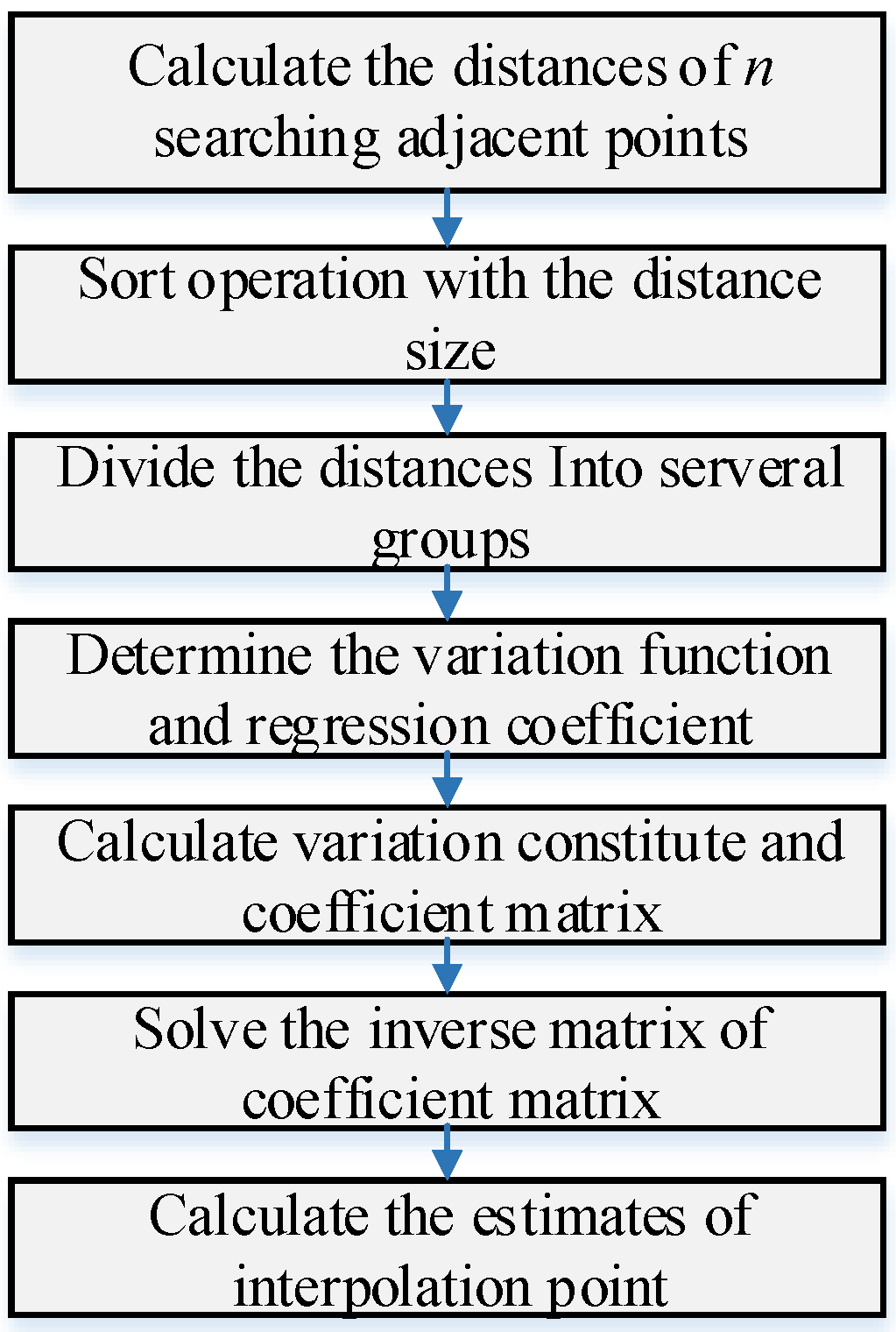
In particular, Step (2) and Step (3) are used to provide the known points and the plane coordinates’ information for the points that need to be inserted, while Step (4) is the main calculation component of the serial universal kriging algorithm. In fact, the implementation of Step (4) is complex, and it can be further divided into seven sub-steps (Sub-steps a–g) (Figure 2), as follows.

• Sub-step a: Calculate the distance between a point that needs to be interpolated and its adjacent points (known points, where the sum is n), i.e., $d_1, d_2, \cdots , d_n$.
• Sub-step b: Sort the distance values obtained into ascending order.
• Sub-step c: Divide the sorted values into k groups.
• Sub-step d: Calculate the average distance $\overline{h_i}$ in each group according to their values. The estimated parameters of the variation function are then calculated using Equation (8). According to the selected theoretical mode of the variation function, function fitting is conducted to determine the variation function and the regression coefficient.
• Sub-step e: Place the distance values of the sampling points and the point into the variation function to construct the coefficient matrix.
• Sub-step f: Solve the inverse matrix of the coefficient matrix in Sub-step (e).
• Sub-step g: Calculate the estimated value of the unknown point until all of the points have been processed.

3.2. Hotspot Analysis and the Corresponding Parallelism Approach

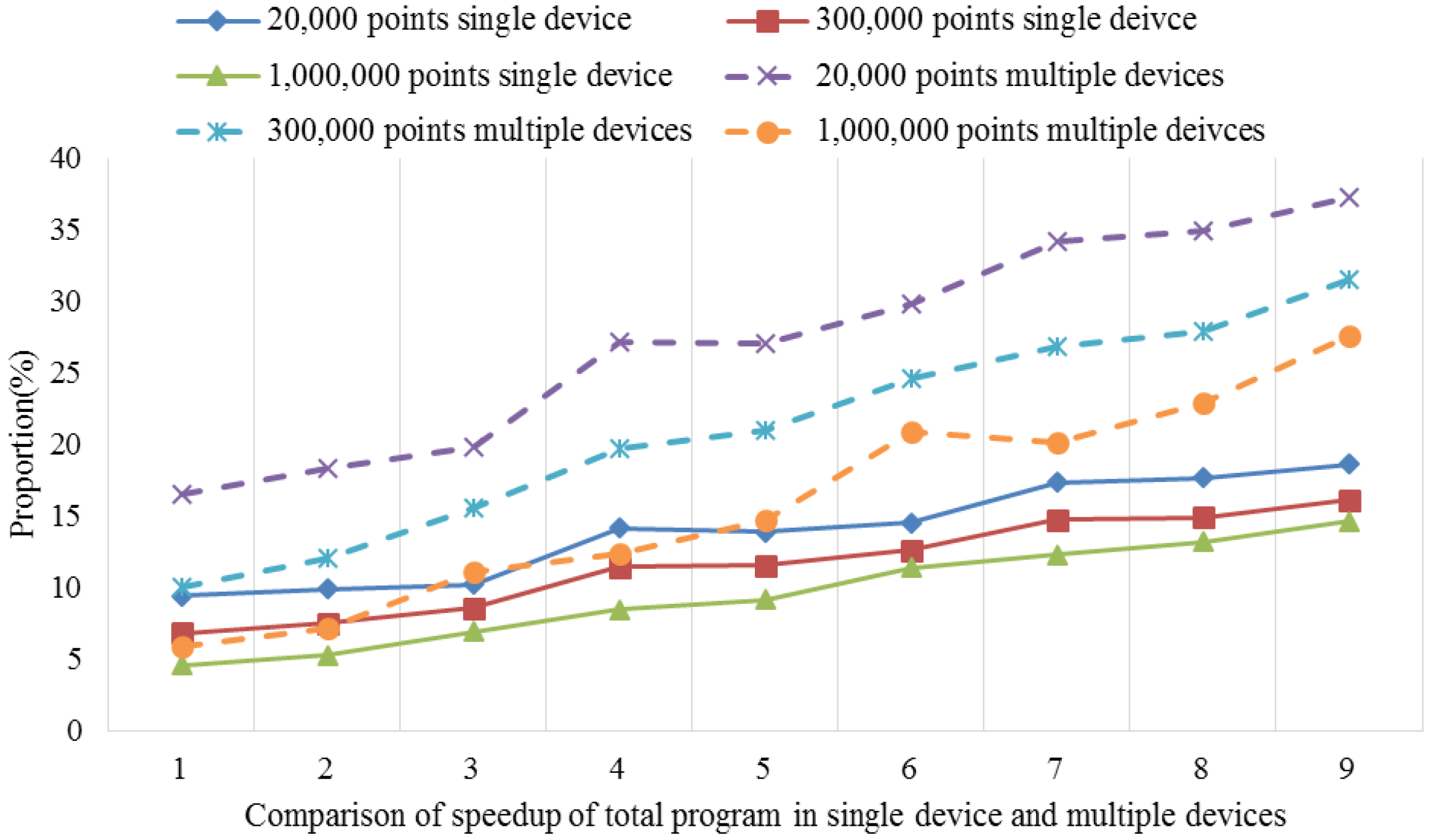
After performing the time consumption analysis using the serial universal kriging algorithm, we found that Step 4, i.e., the kriging interpolation function module, required 85.2%–97.6% of the total elapsed time for different dataset sizes, e.g., small, medium and large datasets. The time consumption percentage was closely related to the number of interpolation points involved and the searches of the adjacent points. Thus, as the number increased, the time consumption percentage tended to increase. For example, the number of search points was set to six in our test, but when this number was 12, which is that used by most real-world applications, the time consumption proportion increased to 90.0%–95.6% with the same dataset groups. Clearly, Step 4 is the hotspot in the serial algorithm.

Therefore, in order to fully accelerate the serial universal kriging algorithm to obtain good performance, the hotspot, i.e., Step 4, requires full consideration. In this step, the calculations of the unknown points are independent of each other, which facilitates the parallelization procedure. Thus, the present study focused mainly on the implementation of parallelism for this step. It should be noted that some specific application issues, such as the estimation of the variogram and the parameters’ settings, are not considered in the parallel implementation. Thus, the parameters used in the proposed parallel algorithm are identified by serial interpolation.

4. Parallel Universal Kriging Algorithm Design and Implementation with OpenCL

4.1. Design and Framework of the Parallel Algorithm

According to the analysis given above, it is clear that Step 4 should be parallelized. However, during the design and implementation of the corresponding efficient parallel algorithm, aspects such as the data structure, data transmission between the host and devices, task partition granularity and load balancing for multiple types of cooperating equipment also require full consideration [43]. Some of these issues are independent of others, whereas there are specific dependencies on others.

To fully consider aspects, such as different platforms, the number of equipped accelerated processors and system memory limitations, we propose the overall framework for the parallel algorithm shown in Figure 3.

According to Figure 3, the framework can be divided into two parts: the host and the device end. Obviously, the main calculation is accomplished in the device. The host only performs control tasks, such as data distribution and collecting results. The host and the device are related by some shared variables.

To develop a parallel algorithm with OpenCL, it is very important to design and implement modules that are highly compliant with the OpenCL framework. When designing the parallel universal kriging algorithm for high performance computing equipment, the main focus is on how to make Step 4, the hotspot, fully fused with the parallel framework in OpenCL. This problem depends mainly on the specific combination, design and implementation of four different programming models: (1) the platform model; (2) the execution model; (3) the memory model; and (4) the programming model. These programming models complement each other, and they are integrated into the overall framework. Thus, other models may be involved when designing and implementing a specific model. According to this rule, in the following, we describe the four models and the proposed framework in detail.

4.2. Platform Model Implementation

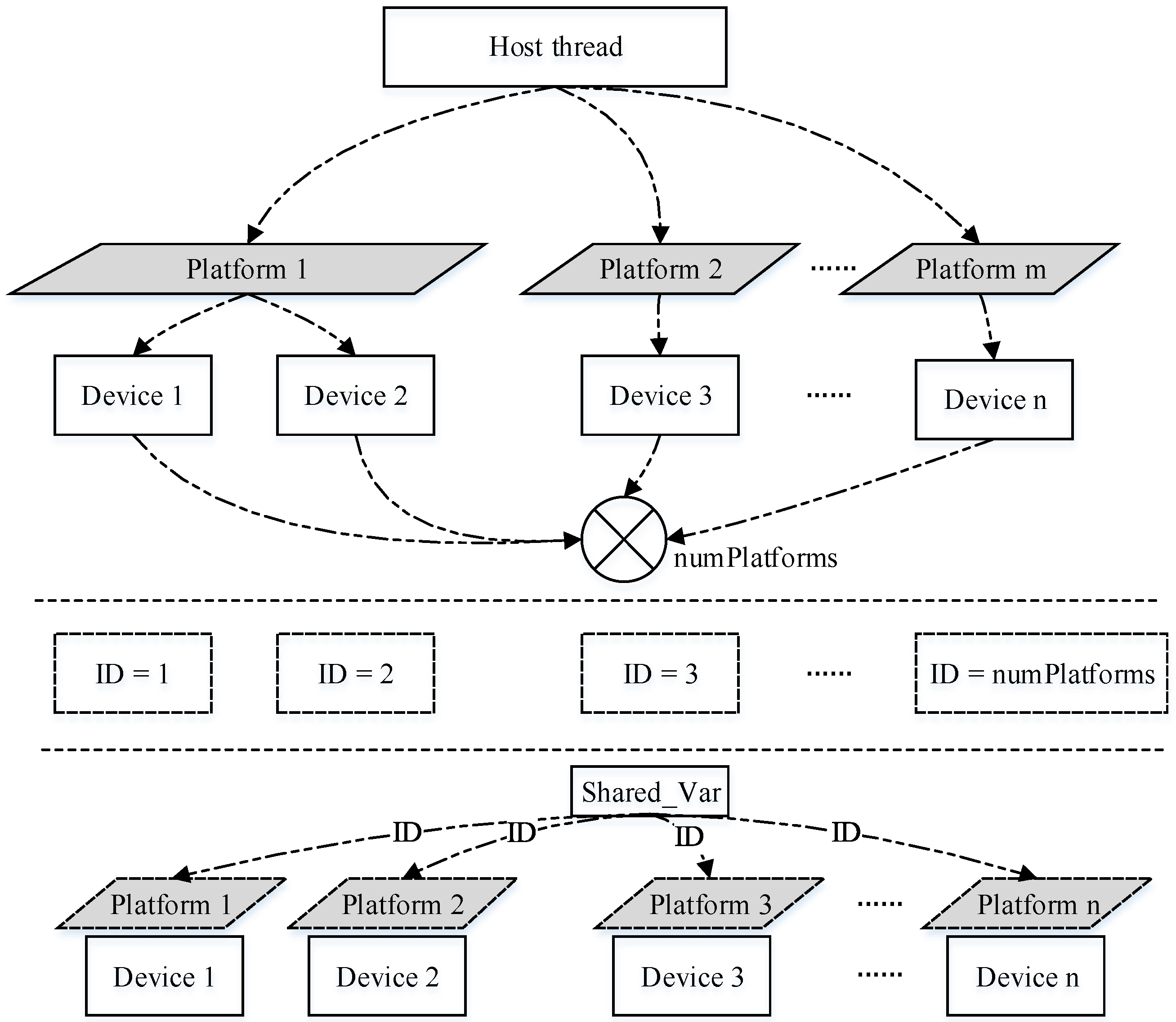
The OpenCL platform model defines a manifestation when using a heterogeneous platform [44]. This blocks the underlying implementation of the equipment, which can only be used by developers in the form of a device, so an additional collaboration pattern between the host and multiple devices needs to be designed. First, the function for creating threads will create suitable threads according to the number of devices. Then, the subsequent steps involve creating platforms, selecting the equipment and creating buffers. Thus, the devices can complete all of the computing tasks cooperatively, and the corresponding implementation is shown in Figure 4.

In Figure 4, the main thread shares information with its child threads. The information includes the task assignment information, platform information pointing to the current equipment and variable information for the insertion time shared by threads. The main thread first obtains the number of available platforms and the devices on each platform, before calculating the total number of all available devices. Next, an equipotent number of threads is created, and some shared variables that transform information with child threads are constructed. Thus, the device ID number stored in the variables shared by each piece of equipment is initialized. Subsequently, the child threads perform operations to recreate the platforms, and they can obtain the corresponding device information given by the main threads.

In the following experiments, we employed two heterogeneous computing platforms: a GPU platform equipped with two GPU cards and an Intel Xeon Phi platform equipped with three MIC cards. In general, a similar procedure was followed to implement the platforms. In the GPU computing platforms, the two GPU cards were treated as OpenCL devices. First, the main process was created in the host end, where its responsibility was to manage the OpenCL platforms and OpenCL devices. Next, two sub-processes were created after the main process found these two OpenCL devices, which mainly operated after the OpenCL device’s initialization. The initialization process mainly comprised context creation, buffer creation, command queue creation, program creation and setting the kernel parameters. Finally, the parallel algorithm sent the kernel and the corresponding data to the appropriate devices, as described above.

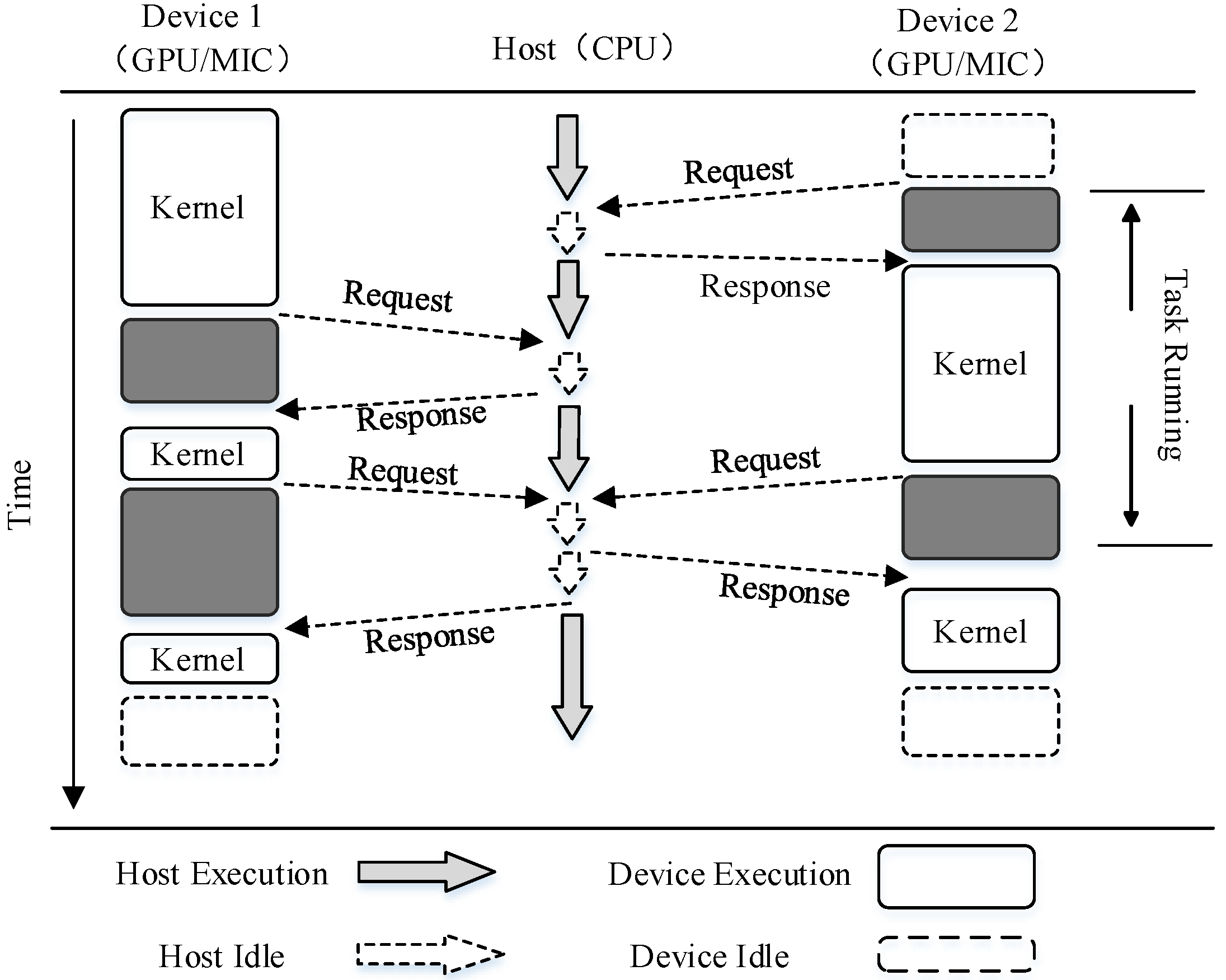
4.3. Execution Model Implementation

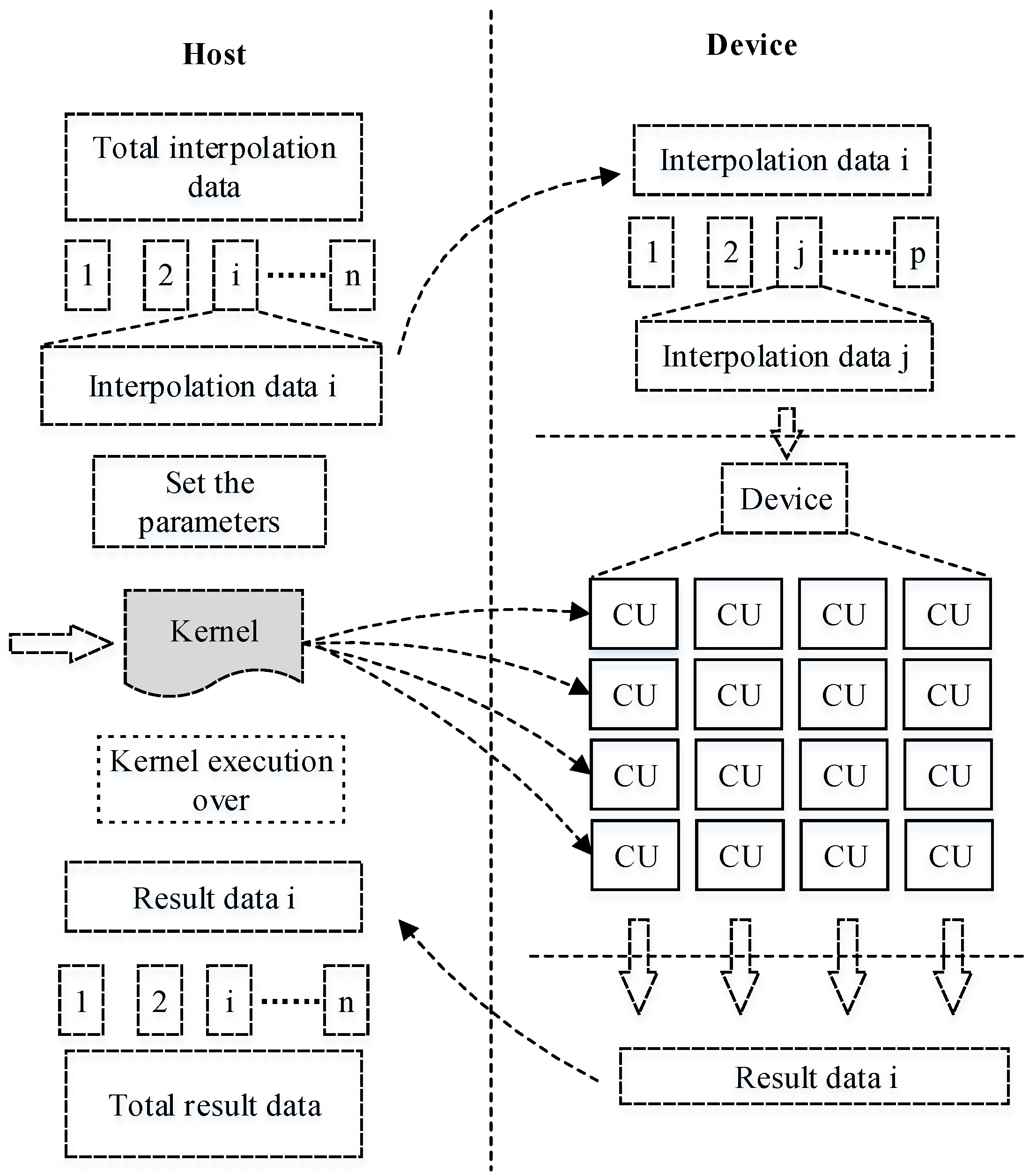
The OpenCL execution model defines the method for executing the kernel function that runs on equipment supporting OpenCL. The OpenCL application comprises two parts: the host machine program and one or more kernels. However, the OpenCL execution model does not define the details of the host machine program. Thus, when there are multiple devices, meticulous work is still required by the developer to divide the workload and to design the tasks collaboratively. In this study, the kernel function was transformed from the part of the serial universal kriging function that needs to be parallelized. When using the data decomposition parallelism method, the host device distributes the kernel function programs to every device (in this case, Computing Units (CUs)). These kernel programs were executed by their corresponding threads; in fact, these threads were created by the host (see Figure 5). It should be noted that the calculations for every unknown point are independent of each other, so there was no need to consider the communication among the kernels or threads.

As shown in Figure 5, the calculation can be completed at one time for a small dataset. The process includes operations, such as data filling, computing and retrieving results. Given that fairly large datasets need to be calculated, it is useful to employ a loop operation to perform the task due to memory limitations. In this case, the data are first divided into n groups according to the memory capacity and the number of CUs (shown on the left in Figure 5). Each group, e.g., group i, is transformed into the devices during an iteration and then decomposed into p portions, which are suitable for calculation by one CU. In this manner, these operations can be repeated many times during one iteration to process large amounts of data. In addition, the host must formulate the distribution of data over multiple devices to ensure the orderly processing of data.

4.4. Memory Model Implementation

The memory model represents how OpenCL divides the memory among the host and the devices for data interactions, where we use the memory object to complete data transmission. In this study, the problem of memory implementation has two aspects: (1) memory mode implementation on the host; and (2) memory mode implementation on computing devices; which are described separately in the following.

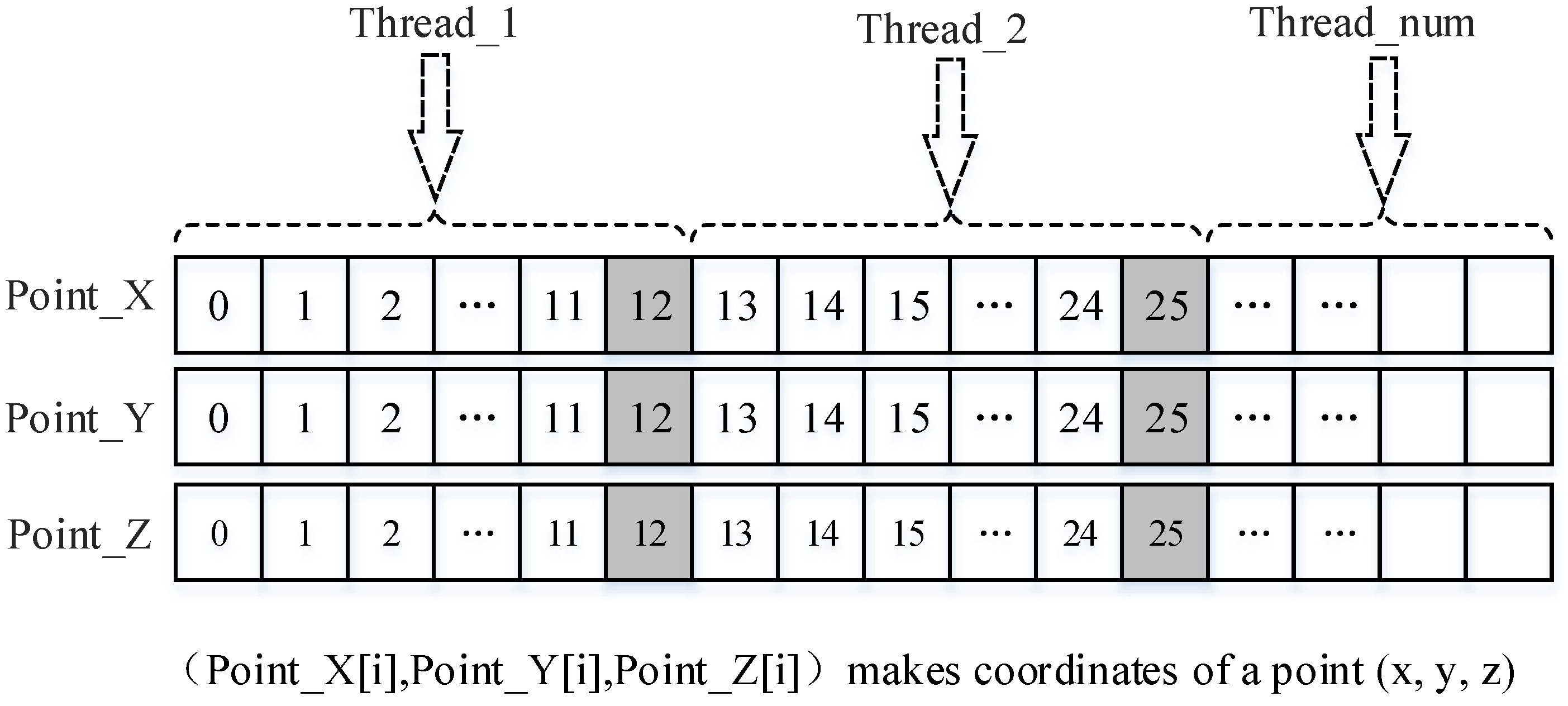
• Memory mode implementation on the host: In the host, the three-dimensional coordinate information for the interpolation data points is read into the system memory first. The array size is determined by the number of points n_points, which is pre-read from the Shapefile formatted file. Next, the number of units that need to be interpolated is created according to the number of parallel threads and the size of memory that can be used by the operating system. The size of the interpolation units is search_n+1, where search_n units are stored with the data information of the search_n neighboring points for the last point that needs to be interpolated. The organization of the data structure for the interpolation unit in each thread is shown in Figure 6.

To avoid wasting time on frequent memory allocation and deallocation, as well as the problem of memory shortages in the computing devices, the memory should be controlled to a certain degree while interpolating. In this study, the maximum limit is $V$, which is determined by controlling the memory percentage or giving a specific size. The optimization code is described as follows.

MAX_MEM_FOR_DATA_STRUCT=1*1024*1024; // Memory is set to 1 MB in the default calculation method

MAX_MEM_FOR_DATA_STRUCT=s_info.totalram*Ration; // Use the memory usage percentage controlling method

Finally, buffers are constructed by the corresponding threads in each device. Thus, operations such as transferring the interpolation data unit to the buffer and sending back the results can be processed continuously. The transmission of data between the master and equipment is completed over several time iterations.

2.

Memory mode implementation on computing devices: the data units that need to be processed can be shared in the form of a global memory between the kernel function and the kernel calling function. The function located on computing devices defines some variables in the form of a private memory to complete data processing in the devices.

Large amounts of data are involved in massive data processing application, where a large number of threads run on the computing devices, so the shared memory and private memory become valuable because these resources are usually limited on hardware. Therefore, we employ a method that directly reads and writes the global variable several times, rather than loading all of the interpolation data from the global variable into the devices each time. This optimization method will affect the processing speed to some extent, but it increases the number of threads that can be run on the devices at the same time, thereby improving the overall performance.

4.5. Programming Model Implementation

The programming model determines the operational strategy that allows the algorithm to be parallelized and to run on OpenCL devices. There are two different programming models in OpenCL: tasks in parallel and data in parallel [39]. It is important to apply the most suitable mode for this algorithm.

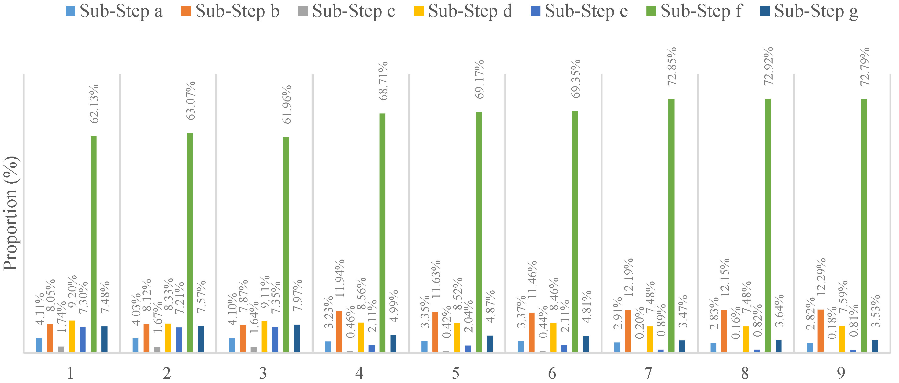
Based on Section 3.1.2, when implementing the parallel universal kriging algorithm, the key step is to parallelize Step 4, which is implemented by the universal kriging function. This function also has seven sub-steps (a–g), which represent operations such as sorting, grouping and calculating the matrix inversion. According to the analyses of the time consumed by every sub-step using a professional performance analyzer, the results for different dataset sizes with various setting parameters are illustrated in Figure 7.

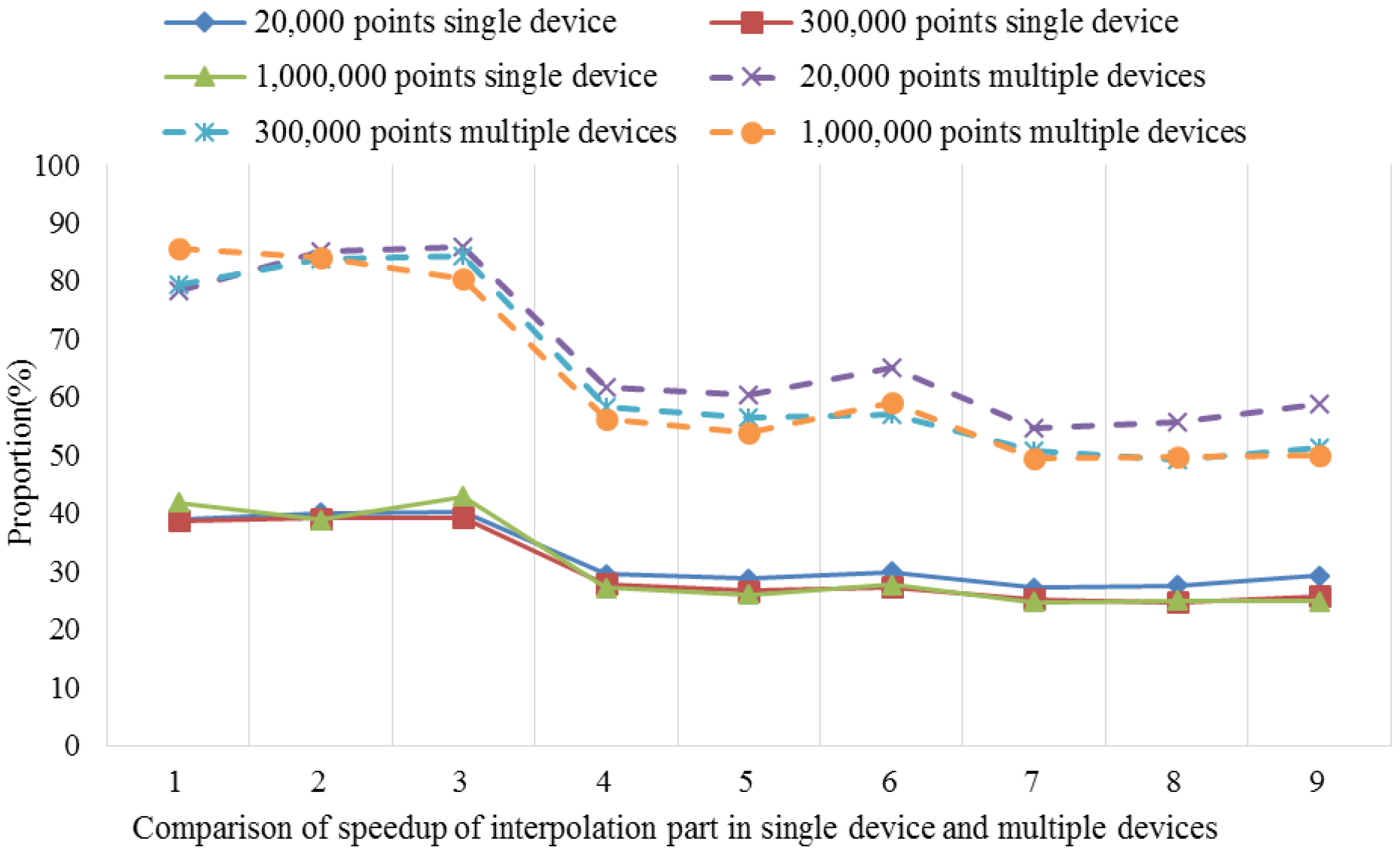
Figure 7 shows that the matrix inversion calculation procedure accounts for 61.9%–72.9% of the runtime for the serial algorithm, which is the highest proportion among all of the sub-steps, and it contains no other steps, such as data reading or searching for adjacent points. However, if we regard this step as the hotspot, the acceleration effect will be very limited. In addition, there are dependencies among other steps, so the task level parallelization mode is not suitable for this algorithm. By contrast, the data that need to be processed can be executed in parallel using the designed structure, where each work-item does not require interactions with other data and there are no data dependencies. Thus, this is the most suitable level for data parallelization. We use this form of data parallelization to implement universal kriging algorithm parallelization (as shown in Figure 3).

4.6. Load Balancing Strategy for Multiple Devices

The task partition granularity and the load-balancing problem must be addressed when there are multiple computing devices. The main thread needs to distribute the overall task to multiple devices for processing, before collecting and combining the computing results to obtain the final SI results. Based on our experimental verification, the parallel algorithm uses a strategy that divides the specific memory according to the average number of equipment, where it considers the maximum number of points that the memory can allow for insertion as the parallelism granularity. In addition, we use the lock mechanism to implement the dynamic load-balancing strategy to compute the task distribution schedule. The detailed implementation of the load-balancing scheduling strategy is illustrated in Figure 8.

5. Experiments and Analysis

5.1. Configuration of the Experimental Environment

We performed experiments on two types of platform: (1) a GPU-based platform; and (2) an Intel Xeon Phi-based platform. The hardware configuration is shown in

Table 1. Detailed configurations of the experimental platforms.

Platform	Hardware Configuration		Software Configuration
Shelob	CPU	Intel(R) E5-2670 CPU @ 2.60 GHz	Linux shelob1 2.6.32-358.23.2.el6.x86_64 OpenCL 1.2 LINUX gdal-1.10.1, proj-4.8.0, geos-3.4.2
		Processor number: 16
		Device global memory: 64,398 MB
		Cache size: 20,480 KB
	GPU	Tesla K20Xm
		Shading Units: 2688
		Device global memory: 5759 MB
		Device number: 2
Tsinghua Intel Xeon Phi	CPU	Intel(R) Xeon(R) CPU E5-2697 v2 @ 2.70 GHz	Linux Tsinghua3MIC 2.6.32-358.el6.x86_64 OpenCL 1.2 LINUX gdal-1.10.1, proj-4.8.0, geos-3.4.2
		Processor number: 24
		Device global memory: 64,390 MB
		Cache size: 30,720 KB
	MIC	Intel(R) Many Integrated Core Acceleration Card
		Core number: 60
		Device global memory: 5773 MB
		Device number: 3

. There were differences in the hardware architecture and design of these two platforms. In these experiments, we aimed to determine the differences in the acceleration obtained and the heterogeneity of the parallel algorithm on different heterogeneous computing platforms.

5.2. Experimental Methodology and Procedure

In the design of the experiments, we considered the following features.

• The difference in performance on various heterogeneous computing platforms also reflects the parallel algorithm’s cross-platform capability.
• Each heterogeneous computing platform was equipped with several acceleration cards, i.e., Shelob had two GPU cards and Tsinghua Intel Xeon Phi three MIC cards, so there may have been differences due to the hardware employed.
• The created threads’ number could be varied, and thus, we investigated how to choose the most suitable number for the experiments.
• The experimental datasets differed in size, i.e., the number of discrete points that required interpolation differed in scale.
• The parameters’ setting used by the algorithm could influence the performance, e.g., the output image pixel size and the number of neighboring points searched.
• To address the issues defined above, we employed the following experimental design.

• The experiments were divided into two groups according to the number of accelerator cards. The first used a single card on each heterogeneous computing platform, and the second used all of the accelerator cards.
• In each experimental group, a suitable number of threads was determined for each computing platform. The datasets differed in size, and the parameters in the algorithm were also changed in each experiment.

In order to assess the differences in performance, the sequential and parallel algorithms were tested in experiments. For the parallel algorithm, the number of threads created T was set to the integral multiple times the number of cores provided by the platform. However, the final number of threads depended on the length of time elapsed. Thus, the hardware’s performance could be utilized to the maximum degree. According to different experiments using various datasets, the numbers of threads with the shortest elapsed time were 26,880 for Shelob and 24,000 for the Intel Xeon Phi platform.

In order to verify the correctness of the parallel program and the acceleration performance, we used several datasets with different sizes to assess the sequential and parallel algorithms. Detailed information related to the datasets is provided in

Table 2. Details of the datasets used in the experiments.

Data Sizes	Data Attributes	Data Sources
Small Dataset	Discrete points’ number: 23,447; saved with Shapefile format; file size is 642 KB.	Contour line generated parameter set to 250 m.
Medium Dataset	Discrete points’ number: 300,431; saved with Shapefile format; file size is 8.02 MB.	Contour line generated parameter set to 20 m.
Large Dataset	Discrete points’ number: 999,894; saved with Shapefile format; file size is 26.7 MB.	Contour line generated parameter set to 6 m.

.

Table 2 shows that three groups of datasets were generated from the original image called srtm_41_14.tif (download from srtm.csi.cgiar.org) with serial analysis operations, such as contour line generation and lining objects to points using ArcGIS software. According to Table 2, the number of points in the small, medium and large datasets could be assigned to three different scales: 20 thousand, 300 thousand and one million, respectively.

To run the parallel algorithm on these heterogeneous computing platforms, we used the following command line:

./kriging -d ./data_file/little/Export_Output_little_250.shp -p 0.001 -n 6

where “-d” is the path of the input dataset that needs to be interpolated by the universal kriging algorithm, “-p” is the pixel size for the generated output image and “-n” indicates the number of search points.

We used the speedup to evaluate the performance of the proposed parallel algorithm, which is the most popular index for this purpose. The speedup $S_p$ is defined as follows:

$$S_p=\frac{T_1}{T_p}$$

(9)

where $T_1$ represents the execution time of the serial program and $T_p$ is the execution time of the parallel algorithm with p processors. In this study, the parallel universal kriging algorithm was influenced by different factors, such as the dataset size and the parameter settings. In order to determine the differences in performance under various conditions, we calculated several speedup values in this experiment. First, according to Equation (9), we calculated the speedup of the entire parallel algorithm and the specific speedup only for the UKIFM part. Second, the relative time consumption by the hotspot changed due to various factors, so we also calculated the current theoretical speedup. The theoretical speedup was calculated using Amdahl’s law [45].

$$Speedup\le \frac{1}{\left(1-pctPar\right)+\frac{pctPar}{p}}$$

(10)

For the inequality, $pctPar$ indicates the percentage of the serial program that needs to be parallelized, and the number of threads/cores is p. When p reaches the highest value in theory, the acceleration limitation equation for the program is as follows.

$$Speedup\le \frac{1}{\left(1-pctPar\right)}$$

(11)

For simplicity, we use $Speedu{p}_A$, $Speedu{p}_I$ and $Speedu{p}_T$ to represent the aforementioned speedup values, respectively.

5.3. Experiment Results and Analysis

5.3.1. Test Results with a Single Computing Device

Table 3. Speedup obtained with a single card on Shelob (small dataset).

$Speedup$	Small Dataset
	n = 6			n = 12			n = 18
	>p	=p	<p	>p	=p	<p	>p	=p	<p
$Speedu{p}_I$	38.85	40.05	40.13	29.42	28.64	29.81	27.10	27.58	29.20
$Speedu{p}_A$	9.41	9.91	10.23	14.17	13.9	14.52	17.35	17.69	18.64
$Speedu{p}_T$	9.43	10.83	10.94	23.47	22.68	23.28	41.15	40.98	40.5

,

Table 4. Speedup obtained with a single card on Shelob (medium dataset).

$Speedup$	Medium Dataset
	n = 6			n = 12			n = 18
	>p	=p	<p	>p	=p	<p	>p	=p	<p
$Speedu{p}_I$	38.70	39.11	39.17	27.82	26.64	27.23	25.12	24.60	25.68
$Speedu{p}_A$	6.81	7.54	8.58	11.47	11.57	12.6	14.77	14.91	16.13
$Speedu{p}_T$	6.83	7.97	9.28	16.55	17.86	19.63	29.65	30.74	34.96

and

Table 5. Speedup obtained with a single card on Shelob (large dataset).

$Speedup$	Large Dataset
	n = 6			n = 12			n = 18
	>p	=p	<p	>p	=p	<p	>p	=p	<p
$Speedu{p}_I$	41.79	38.79	42.85	27.11	26.01	27.64	24.72	24.86	24.84
$Speedu{p}_A$	4.59	5.3	6.95	8.5	9.18	11.42	12.29	13.22	14.66
$Speedu{p}_T$	4.68	5.35	6.99	11.11	12.24	16.31	21.23	23.98	28.6

show the experimental results obtained using a single accelerator device with three different dataset sizes on the Shelob platform. For the same conditions, the experimental results obtained on the Intel Xeon Phi platform are given in

Table 6. Speedup obtained with a single card on Intel Xeon Phi (small dataset).

$Speedup$	Small Dataset
	n = 6			n = 12			n = 18
	>p	=p	<p	>p	=p	<p	>p	=p	<p
$Speedu{p}_I$	11.43	11.30	11.42	10.96	10.87	10.76	11.77	11.67	11.66
$Speedu{p}_A$	5.02	5.74	6.09	7.46	7.53	7.74	9.18	9.23	9.37
$Speedu{p}_T$	10.64	10.66	11.15	21.26	22.89	22.89	37.33	38.24	40.15

,

Table 7. Speedup obtained with a single card on Intel Xeon Phi (medium dataset).

$Speedup$	Medium Dataset
	n = 6			n = 12			n = 18
	>p	=p	<p	>p	=p	<p	>p	=p	<p
$Speedu{p}_I$	11.55	11.59	11.56	11.00	11.03	11.00	11.77	11.79	11.72
$Speedu{p}_A$	4.39	4.87	5.57	6.61	7.02	7.43	8.53	8.8	9.05
$Speedu{p}_T$	6.84	7.67	8.91	15.52	16.8	19.22	28.04	30.15	33.56

and

Table 8. Speedup obtained with a single card on Intel Xeon Phi (large dataset).

$Speedup$	Large Dataset
	n = 6			n = 12			n = 18
	>p	=p	<p	>p	=p	<p	>p	=p	<p
$Speedu{p}_I$	11.50	11.58	11.62	10.91	10.92	10.96	11.78	11.66	11.72
$Speedu{p}_A$	2.91	3.53	4.57	5.35	5.94	6.78	7.5	7.93	8.66
$Speedu{p}_T$	4.21	5.11	6.95	9.95	11.79	15.27	18.54	22.85	27.99

. In these tables, n is the parameter setting for the neighborhood search number and p is the original spatial resolution value, where the output image’s resolution was set as less than, equal to or greater than p in this experiment. The data used to calculate $Speedu{p}_T$ came from the serial algorithm’s hotspot detection.

Table 3, Table 4 and Table 5 show the following. (1) In general, the parallel algorithm obtained good acceleration performance, and it could reduce the processing time to a certain degree. In particular, when we only considered the universal kriging interpolation part, the highest speedup reached up to 40×, but the value of $Speedu{p}_I$ decreased as the number of search points increased. (2) $Speedu{p}_I$ and $Speedu{p}_T$ also decreased as the dataset size increased. In theory, these decreasing trends were caused mainly by the need for more registers in each thread when the thread number was fixed. In these conditions, the parallelism granularity decreased and a longer running time was required.

Table 6, Table 7 and Table 8 show the following. (1) The speedup exhibited a similar trend to that on Shelob. (2) The speedup obtained on the Intel Xeon Phi platform was far less than that on Shelob. This was due mainly to differences in the computing capacity of the MIC card and NVIDIA card. The peak number for the MIC card was 508 GFLOPS (giga floating point operations per second) in theory, whereas that for the NVIDIA card was 1311 GFLOPS, and thus, it was more powerful than the former.

5.3.2. Test Results with Multiple Computing Devices

When all of the accelerator cards were used, i.e., two GPU cards on Shelob and three MIC cards on Intel Xeon Phi, load balancing also played a role. In the same manner as the experiments described above, we compared the $Speedu{p}_I$ and $Speedu{p}_A$ calculated with different accelerator cards. Figure 9 and Figure 10 compared the speedup obtained on the Shelob platform.

Using multiple devices, the speedup was almost doubled in both cases. Moreover, the speedup ratio increased when the dataset size was larger.

Figure 11 and Figure 12 compare the speedup results obtained with a single card and multiple cards on the Intel Xeon Phi platform.

Similarly, compared to a single device, $Speedu{p}_I$ and $Speedu{p}_A$ increased by three times, which was the number of multiple devices. In addition, the speedup ratio also increased.

Therefore, the results of these experiments demonstrate that the speedup changed in a linear manner compared to that on a single device when we used multiple devices, which verified that our load-balancing strategy was useful and effective.

6. Conclusions and Future Directions

In this study, we focused mainly on the design and implementation of a parallel universal kriging interpolation algorithm using the OpenCL programming model on heterogeneous platforms. In the future, the source codes will be made available on GitHub. Based on the experimental results, we can make the following conclusions.

• The universal kriging interpolation algorithm developed with OpenCL could run on different heterogeneous computing platforms without any modifications, i.e., GPU-based or MIC-based platforms. Therefore, the proposed method has satisfactory cross-platform capability.
• Compared to the serial algorithm that runs only on the CPU platform, the parallel universal kriging algorithm, especially its interpolation calculation part, can achieve a good acceleration ratio on different heterogeneous platforms.
• The use of multiple computing devices, i.e., more GPU/MIC cards for computation, obtained almost linear increases in the acceleration ratio and better performance than single computing devices. However, the OpenCL-based heterogeneous computing approach also has its weaknesses, including complex programming, high memory demands, little usage of recursive functions and relatively low efficiency compared to CUDA.

In addition, there is still the possibility of further optimization of the proposed parallel universal kriging program. For example, using a larger interpolation scale, the step employed to search for neighboring points in the parallel program would gradually become the major hotspot. Therefore, this hotspot requires greater consideration to further enhance the performance of the parallel algorithm.

References

1. Li, J. A Review of Spatial Interpolation Methods for Environmental Scientists; Geoscience Australia: Canberra, Australia, 2008. [Google Scholar]
2. Myers, D.E.; Begovich, C.L.; Butz, T.R.; Kane, V.E. Variogram models for regional ground water geochemical data. Math. Geol. 1982, 14, 629–644. [Google Scholar] [CrossRef]
3. Ozelkan, E.; Chen, G.; Ustundag, B.B. Spatial estimation of wind speed: A new integrative model using inverse distance weighting and power law. Int J Digit Earth. 2016. [Google Scholar] [CrossRef]
4. Bhattacharjee, S.; Mitra, P.; Ghosh, S.K. Spatial interpolation to predict missing attributes in GIS using semantic kriging. IEEE Ttrans. Geosci. Remote Sens. 2014, 52, 4771–4780. [Google Scholar] [CrossRef]
5. Rossi, R.E.; Dungan, J.L.; Beck, L.R. Kriging in the shadows: Geostatistical interpolation for remote sensing. Remote Sens. Environ. 1994, 49, 32–40. [Google Scholar] [CrossRef]
6. Zhang, X.; Jiang, H.; Zhou, G.; Xiao, Z.; Zhang, Z. Geostatistical interpolation of missing data and downscaling of spatial resolution for remotely sensed atmospheric methane column concentrations. Int. J. Remote Sens. 2012, 33, 120–134. [Google Scholar] [CrossRef]
7. Carr, J.R.; Deng, E.D.; Glass, C.E. An application of disjunctive kriging for earthquake ground motion estimation. Math. Geol. 1986, 18, 197–213. [Google Scholar] [CrossRef]
8. Dag, A.; Ozdemir, A.C. A comparative study for 3D surface modeling of coal deposit by spatial interpolation approaches. Resour. Geol. 2013, 63, 394–403. [Google Scholar] [CrossRef]
9. Reed, P.; Minsker, B.; Valocchi, A.J. Cost-effective long-term groundwater monitoring design using a genetic algorithm and global mass interpolation. Water Resour Res. Water Resour. Res. 2000, 36, 3731–3741. [Google Scholar] [CrossRef]
10. Cressie, N.; Kang, E.L. High-Resolution digital soil mapping: Kriging for very large datasets. In Proximal Soil Sensing; Springer: Dordrecht, The Netherlands, 2010; pp. 49–63. [Google Scholar]
11. Kao, C.S. Automated interpolation of two-dimensional seismic grids into three-dimensional data volume. Geophysics 1990, 55, 433–442. [Google Scholar] [CrossRef]
12. Sahlin, J.; Mostafavi, M.A.; Forest, A.; Babin, M. Assessment of 3D Spatial interpolation methods for study of the marine pelagic environment. Mar. Geodes. 2014, 37, 238–266. [Google Scholar] [CrossRef]
13. Loubier, J.C. Optimizing the interpolation of temperatures by GIS: A space analysis approach. In Spatial Interpolation for Climate Data; ISTE: London, UK, 2010; pp. 97–107. [Google Scholar]
14. Chang, C.L.; Lo, S.L.; Yu, S.L. The parameter optimization in the inverse distance method by genetic algorithm for estimating precipitation. Environ. Monit. Assess. 2006, 117, 145–155. [Google Scholar] [CrossRef] [PubMed]
15. Jeffrey, S.J.; Carter, J.O.; Moodie, K.B.; Beswick, A.R. Using spatial interpolation to construct a comprehensive archive of Australian climate data. Environ. Model. Softw. 2001, 16, 309–330. [Google Scholar] [CrossRef]
16. Huang, F.; Liu, D.; Tan, X.; Wang, J.; Chen, Y.; He, B. Explorations of the implementation of a parallel IDW interpolation algorithm in a Linux cluster-based parallel GIS. Comput. Geosci. 2011, 37, 426–434. [Google Scholar] [CrossRef]
17. Cressie, N.; Johannesson, G. Fixed rank kriging for very large spatial data sets. J. R. Stati. Soc. 2008, 70, 209–226. [Google Scholar] [CrossRef]
18. Ingram, B.; Dan, C. Parallel geostatistics for sparse and dense datasets. Quant. Geol. Geostat. 2010, 16, 371–381. [Google Scholar]
19. Armstrong, M.P.; Marciano, R. Massively parallel processing of spatial statistics. Int. J. Geogr. Inf. Sci. 1995, 9, 169–189. [Google Scholar] [CrossRef]
20. Gajraj, A.; Joubert, W.; Jones, J. A Parallel Implementation of Kriging with a Trend. Available online: http://www.osti.gov/scitech/servlets/purl/544698-DhOroO/webviewable/ (accessed on 10 June 2015).
21. Hawick, K.A.; Coddington, P.D.; James, H.A. Distributed frameworks and parallel algorithms for processing large-scale geographic data. Parall. Comput. 2003, 29, 1297–1333. [Google Scholar] [CrossRef]
22. Guan, X.; Wu, H. Leveraging the power of multi-core platforms for large-scale geospatial data processing: Exemplified by generating DEM from massive LiDAR point clouds. Comput. Geosci. 2010, 36, 1276–1282. [Google Scholar] [CrossRef]
23. Wang, S.; Armstrong, M.P. A quadtree approach to domain decomposition for spatial interpolation in Grid computing environments. Parall. Comput. 2003, 29, 1481–1504. [Google Scholar] [CrossRef]
24. Kerry, K.E.; Hawick, K.A. Kriging interpolation on high-performance computers. In High-Performance Computing and Networking; Springer: Berlin, Germany, 1998; pp. 429–438. [Google Scholar]
25. Pedelty, J.A.; Morisette, J.T.; Smith, J.A.; Schnase, J.L.; Crosier, C.S.; Stohlgren, T.J. High Performance Geostatistical Modeling of Biospheric Resources. Available online: https://esto.nasa.gov/conferences/estc2003/papers/A4P4(Schnase).pdf (accessed on 10 June 2015).
26. Valentini, G.L.; Lassonde, W.; Khan, S.U.; Min-Allah, N.; Madani, S.A.; Li, J.; Zhang, L.; Wang, L.; Ghani, N.; Kolodziej, J. An overview of energy efficiency techniques in cluster computing systems. Cluster Comput. 2011, 16, 1–13. [Google Scholar] [CrossRef]
27. Strzelczyk, J.; Porzycka, S.; Lesniak, A. Analysis of ground deformations based on parallel geostatistical computations of PSInSAR data. In Proceedings of the International Conference on Geoinformatics, Fairfax, VA, USA, 12–14 August 2009; pp. 195–206.
28. Li, J.; Jiang, Y.; Yang, C.; Huang, Q.; Rice, M. Visualizing 3D/4D environmental data using many-core graphics processing units (GPUs) and multi-core central processing units (CPUs). Comput. Geosci. 2013, 59, 78–89. [Google Scholar] [CrossRef]
29. Liu, P.; Yuan, T.; Yan, M.A.; Wang, L.; Liu, D.; Yue, S.; Kołodziej, J. Parallel processing of massive remote sensing images in a GPU architecture. Comput. Inform. 2014, 33, 197–217. [Google Scholar]
30. Xue, W.; Yang, C.; Fu, H.; Wang, X.; Xu, Y.; Liao, J.; Gan, L.; Lu, Y.; Ranjan, R.; Wang, L. Ultra-scalable CPU-MIC acceleration of mesoscale atmospheric modeling on Tianhe-2. IEEE Trans. Comput. 2015, 64, 2382–2393. [Google Scholar] [CrossRef]
31. Chen, D.; Li, D.; Xiong, M.; Bao, H.; Li, X. GPGPU-aided ensemble empirical-mode decomposition for EEG analysis during anesthesia. IEEE Trans. Inf. Technol. Biomed. 2010, 14, 1417–1427. [Google Scholar] [CrossRef] [PubMed]
32. Cheng, T. Accelerating universal Kriging interpolation algorithm using CUDA-enabled GPU. Comput. Geosci. 2013, 54, 178–183. [Google Scholar] [CrossRef]
33. Heinecke, A.; Klemm, M.; Bungartz, H.J. From GPGPU to Many-core: NVIDIA Fermi and Intel many integrated core architecture. Comput. Sci. Eng. 2012, 14, 78–83. [Google Scholar] [CrossRef]
34. Wang, Y.; Deng, G.; Zhiliang, X.U. Performance optimization methods for boosting MIC-based parallel computing. J. Shenzhen Inst. Inf. Technol. 2013, 11, 87–93. [Google Scholar]
35. Gaster, B.; Howes, L.; Kaeli, D.R.; Mistry, P.; Schaa, D. Heterogeneous Computing with OpenCL; Morgan Kaufmann: Burlington, MA, USA, 2011. [Google Scholar]
36. Bartier, P.M.; Keller, C.P. Multivariate interpolation to incorporate thematic surface data using inverse distance weighting (IDW). Comput. Geosci. 1996, 22, 795–799. [Google Scholar] [CrossRef]
37. Lindholm, E.; Nickolls, J.; Oberman, S.; Montrym, J. NVIDIA Tesla: A unified graphics and computing architecture. IEEE Micro 2008, 28, 39–55. [Google Scholar] [CrossRef]
38. Duran, A.; Klemm, M. The Intel® many integrated core architecture. In Proceedings of the 2012 International Conference on High Performance Computing and Simulation (HPCS), Madrid, Spain, 2–6 July 2012; pp. 365–366.
39. Stone, J.E.; Gohara, D.; Shi, G. OpenCL: A parallel programming standard for heterogeneous computing systems. Comput. Sci. Eng. 2010, 12, 66–73. [Google Scholar] [CrossRef] [PubMed]
40. Chilès, J.P.; Delfiner, P. Geostatistics: Modeling Spatial Uncertainty; John Wiley & Sons, Inc.: New York, NY, USA, 2012. [Google Scholar]
41. Gorsich, D.J.; Genton, M.G. Variogram model selection via nonparametric derivative estimation. Math. Geol. 2000, 32, 249–270. [Google Scholar] [CrossRef]
42. Altman, N.S. An introduction to kernel and nearest-neighbor nonparametric regression. Am. Stat. 1992, 46, 175–185. [Google Scholar]
43. Kirk, D.B.; Hwu, W.M.W. Programming Massively Parallel Processors: A Hands-on Approach; Morgan Kaufmann: Burlington, MA, USA, 2012. [Google Scholar]
44. Tsuchiyama, R.; Nakamura, T.; Lizuka, T.; Asahara, A.; Miki, S.; Tagawa, S. The OpenCL Programming Book; Fixstars Corporation: Tokyo, Japan, 2010. [Google Scholar]
45. Shi, B.Y. Reevaluating Amdahl’s law and Gustafson’s law. Microbiol. Read. Engl. 2010, 160, 113–122. [Google Scholar]
Figure 1. Modules in the serial universal kriging algorithm.
Ijgi 05 00096 g001
Figure 2. Main steps of the universal kriging interpolation function.
Ijgi 05 00096 g002
Figure 3. Overall framework for the parallel universal kriging algorithm implementation.
Ijgi 05 00096 g003
Figure 4. Implementation of the platform model.
Ijgi 05 00096 g004
Figure 5. Overview showing the execution of an OpenCL parallel program.
Ijgi 05 00096 g005
Figure 6. Data organization structure.
Ijgi 05 00096 g006
Figure 7. Time consumption by each sub-step in the universal kriging function.
Ijgi 05 00096 g007
Figure 8. Strategy for load balancing among multiple devices.
Ijgi 05 00096 g008
Figure 9. Comparison of the speedup obtained using single/multiple cards on Shelob ( S p e e d u p I ).
Ijgi 05 00096 g009
Figure 10. Comparison of the speedup obtained using single/multiple cards on Shelob ( S p e e d u p A ).
Ijgi 05 00096 g010
Figure 11. Comparison of the speedup obtained using single/multiple cards on Intel Xeon Phi ( S p e e d u p I ).
Ijgi 05 00096 g011
Figure 12. Comparison of the speedup obtained using single/multiple cards on Intel Xeon Phi ( S p e e d u p A ).
Ijgi 05 00096 g012