Parallel Landscape Driven Data Reduction & Spatial Interpolation Algorithm for Big LiDAR Data

Abstract

Airborne Light Detection and Ranging (LiDAR) topographic data provide highly accurate digital terrain information, which is used widely in applications like creating flood insurance rate maps, forest and tree studies, coastal change mapping, soil and landscape classification, 3D urban modeling, river bank management, agricultural crop studies, etc. In this paper, we focus mainly on the use of LiDAR data in terrain modeling/Digital Elevation Model (DEM) generation. Technological advancements in building LiDAR sensors have enabled highly accurate and highly dense LiDAR point clouds, which have made possible high resolution modeling of terrain surfaces. However, high density data result in massive data volumes, which pose computing issues. Computational time required for dissemination, processing and storage of these data is directly proportional to the volume of the data. We describe a novel technique based on the slope map of the terrain, which addresses the challenging problem in the area of spatial data analysis, of reducing this dense LiDAR data without sacrificing its accuracy. To the best of our knowledge, this is the first ever landscape-driven data reduction algorithm. We also perform an empirical study, which shows that there is no significant loss in accuracy for the DEM generated from a 52% reduced LiDAR dataset generated by our algorithm, compared to the DEM generated from an original, complete LiDAR dataset. For the accuracy of our statistical analysis, we perform Root Mean Square Error (RMSE) comparing all of the grid points of the original DEM to the DEM generated by reduced data, instead of comparing a few random control points. Besides, our multi-core data reduction algorithm is highly scalable. We also describe a modified parallel Inverse Distance Weighted (IDW) spatial interpolation method and show that the DEMs it generates are time-efficient and have better accuracy than the one’s generated by the traditional IDW method.

1. Introduction

1.1. Overview

Airborne Light Detection and Ranging (LiDAR) is one of the most effective means for high density and high accuracy terrain data acquisition. Three-dimensional spatial imaging with LiDAR technology is a powerful remote sensing methodology that can be used to produce detailed maps of objects, surfaces and terrain across widely varying scales [1]. Improved scanning technologies have made it easier to generate massive high density LiDAR point clouds and, therefore, more accurate, compact terrain models and other three-dimensional representations [2]. LiDAR topographic data provide highly accurate digital terrain information, which is widely used in applications, like updating and creating flood insurance rate maps, forest and tree studies, coastal change mapping, soil and landscape classification, 3D urban modeling, river bank management, agricultural crop studies, etc. However, the generation of such improved models from high density and an enormous volume of data imposes great challenges with respect to data storage, processing and manipulation.

Over the last 15 years, use of LiDAR data for generating reliable and accurate Digital Elevation Models (DEMs) is widely used in the geospatial science communities [3]. The accuracy of the generated DEM is directly proportional to the density of the sample terrain LiDAR data used. Hence, strategies to process large volumes of dense LiDAR data without compromising the accuracy are essential. In this paper, we describe a novel algorithmic technique to reduce LiDAR data to achieve an optimal equivalence between the density and volume of data, which facilitates accurate and efficient generation of DEMs. Our algorithm reduces LiDAR points based on the topography, mainly the slope map, of the terrain under consideration. To the best of our knowledge, this is the first ever landscape-driven data reduction technique. We also use parallel programming to exploit the multi-core architecture of CPUs, thus making our algorithm highly scalable and time-efficient.

A natural terrain surface is a continuous surface comprised of infinite points [4]. We use point sampling techniques to approximate the accuracy of the generated DEMs to the required resolutions. The most commonly-used DEMs are the grid DEM, the contour line DEM and the triangular irregular network (TIN) DEM. A grid DEM can be represented as a matrix, having related data points that capture the information of the terrain’s topography. Every grid cell has a value that denotes the elevation for the entire cell [5]. Each of the grid cells get this elevation value by interpolating (approximation procedure) adjacent sampling points. In [6], interpolation is defined as a process of interpreting values at points found in unsampled regions, on the basis of values at points within the confined area of study. Interpolation techniques in grid DEMs are used to determine the terrain height value of a point based on the known elevation values of points in the neighborhood [7]. The quality of the DEMs is evaluated based on the difference between the true and the interpolated value at points in the entire or selected locations [8].

Practically applying spatial interpolation is a computationally-expensive task, and it requires powerful computing resources. Spatial interpolation is applied more to massive data analysis, which requires more processing time. For certain applications, like real-time mapping of terrains, driverless farm vehicles, etc., using a LiDAR sensor on-board is mainly applied on sparse vegetation. Our DEM generation algorithm coupled with our data reduction algorithm has the potential to improve the efficiency for such applications. In this paper, we present a parallel modified IDW spatial interpolation technique, which exploits multiple cores of CPUs to perform computationally better than traditional IDW. We also compare the DEM generated by our algorithm to the one generated by traditional IDW, using validation. Further, we also evaluate the comparison using statistical approaches, like RMSE.

1.2. Related Work

1.2.1. Approaches to Data Reduction

The enhancement in data collection technologies has enabled the generation of massive amounts of data, which poses computing issues when disseminating, processing and storing data. Data are valuable only if they can convey useful information. All of the points in the entire LiDAR point cloud do not provide equally valuable information about the terrain under consideration [9]. In order for a DEM to be useful, it should be of a desired size so that it can be manipulated whenever required within the technology used to render it. This is one of the main challenges in massive geo-spatial data processing: reduce the dataset to attain an optimal balance between the size of the dataset required and the desired resolution. The work described in [10] shows the effects of LiDAR data density on generated DEMs for a range of resolutions. They further showed that LiDAR data can be reduced substantially, yet still be able to generate accurate DEMs for elevation predictions. The effects of LiDAR data density on the accuracy of the generated DEMs and the extent to which LiDAR data can be reduced and still achieve DEMs with the required accuracy is studied in [11]. A method of vertex decimation i.e., selective removal of points from the LiDAR point cloud that do not convey enough information was introduced in [12]. Hegeman et al. proposed a method [13] in which each point was considered for deletion based on the z-variance of the point cloud in the small local region. A variance threshold was initially set up as an input parameter; local regions having z-variance less than the threshold undergo removal of most of their central points. They concluded that, for certain regimes, this point decimation technique performs significantly better than random decimation. Certain data filtering algorithms, like [14,15], focus and perform well on steep, forested areas where other filtering algorithms typically have problems distinguishing between ground returns and off-ground points reflected in the vegetation. However, these approaches are not efficient where there is no or sparse vegetation. For certain applications, like real-time mapping of terrains (farm-land), driverless farm vehicles like (tractor, sower, sprayer, etc.), a harvester with automatic blade-angle setting, etc., using a LiDAR sensor on-board is mainly applied before the emergence of vegetation or with sparse vegetation. The algorithm we present in this paper proves efficient for such applications.

1.2.2. Approaches to Spatial Interpolation

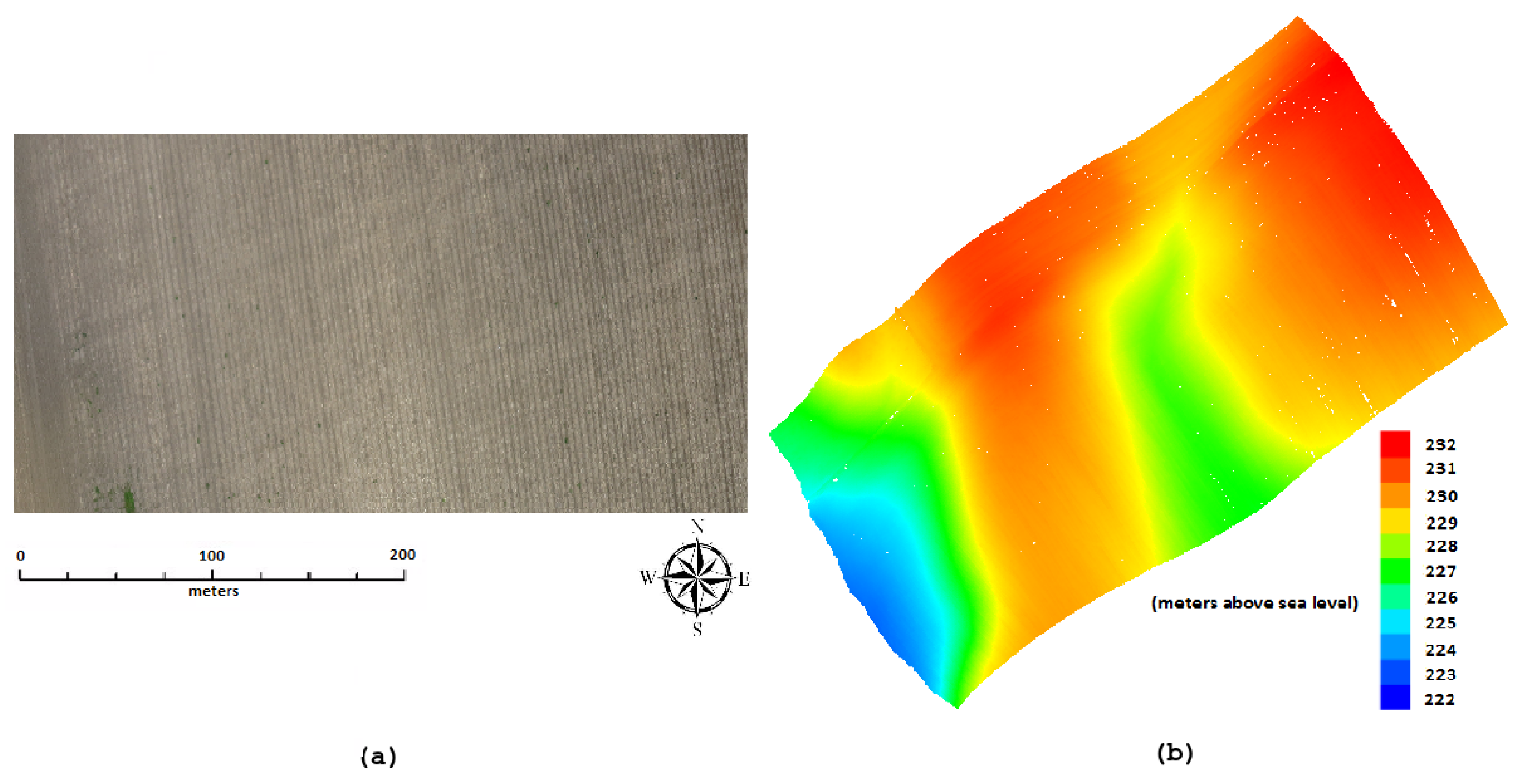
Amongst of all of the spatial interpolation techniques, generating DEMs using grid DEM techniques has more a efficient storage and manipulation scope [4]. DEMs generated using grids introduce errors, since the terrain is represented in a discrete fashion, but the error is comparatively lesser for dense datasets when compared to TIN, kriging, etc. The size of the grid used for generating DEM is directly proportional to the approximation ratio of the terrain surface representation. Since LiDAR data are dense, such limitations of the grid DEM method can be eliminated. The work in [16] studied complex models to generate DEMs resulting from hybrid techniques. However, in practice, all of the DEMs generated from LiDAR are done using grid techniques [17]. Due to the availability of a large variety of interpolation techniques, questions on which is the most appropriate technique for different terrains need to be answered. Empirical studies to answer these questions and to evaluate the effects of various interpolation techniques on DEM quality are shown in [4,18,19]. There does not exist any one interpolation technique that is optimal for all terrain surface data [20]. The IDW interpolation technique is proven to exhibit better performance when the sampled data have high density. Since LiDAR data have high density, IDW is a preferred choice to generate DEMs [21,22].

2. Dataset

The test LiDAR dataset we use for our experiments represents a 300 m $\times 380$ m tile, of a terrain in Iowa. The imagery of the study area is shown in Figure 1a. This LiDAR dataset is interesting because it has a good mix of flat land, land with moderate inclination and steep slopes. Thus, it resembles a real-life terrain, rather than computationally-ideal terrains consisting of just flat land. The slope angle for the entire terrain varies between $0.03$° and $63.18$°. This LiDAR dataset has been collected using Airborne LiDAR by Aerial Services, Inc. (ASI), Iowa, USA. The dataset is comprised of $6.94$ million points, with a point density of approximately 120 points per sq.m. In the experiments, the input files were formatted in ASPRS LAS File Format, Version 1.0. The size of this dataset was $1.5$ GB. Furthermore, for visualization purposes, we converted the input data with extension .LAS to .xyz using LASTools. The LiDAR point cloud for the above data is generated using ArcGIS, ArcMap v$10.3$, as shown in Figure 1b. The spatial resolution of the LiDAR data was estimated to be $0.0254$ m vertically and $0.0254$ m horizontally.

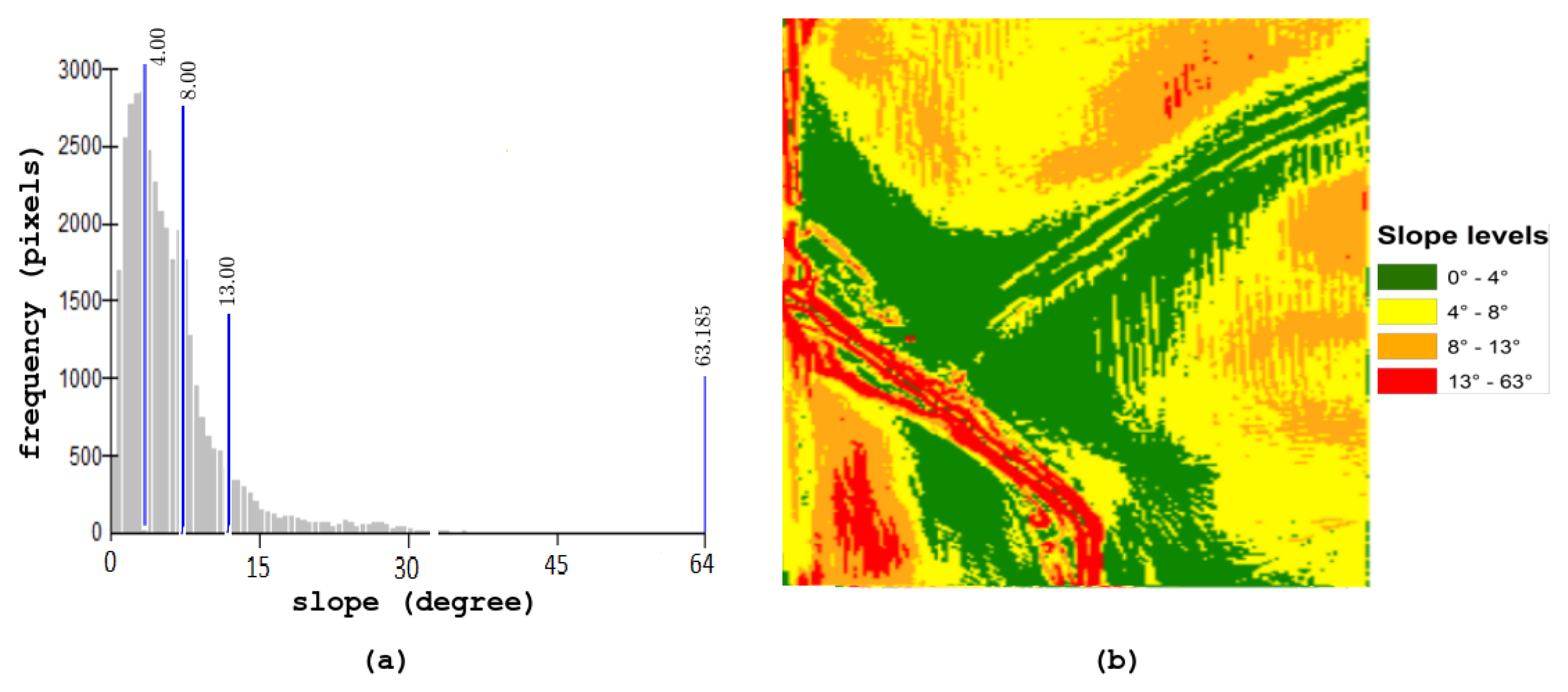
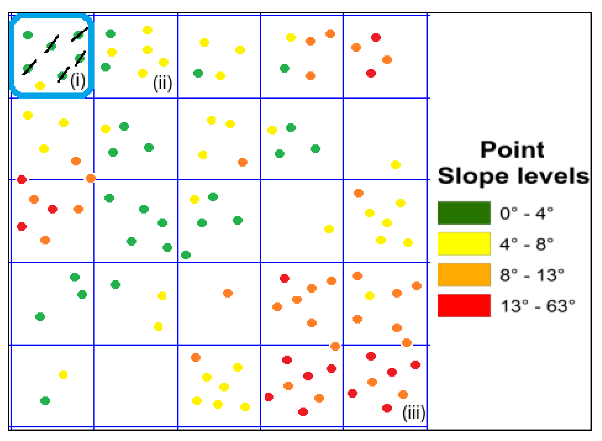
3. Data Reduction Method

3.1. Data Preparation

Initially, we make use of the elevation data available for the study area to generate a slope map. For this paper, we generate this elevation data using LiDAR data that we collected for the entire region. Elevation data are also available freely in the National Elevation Dataset (NED) [23], which is the primary elevation data product of the United States Geological Survey (USGS) and serves as the elevation layer of “The National Map”. The NED provides elevation information for Earth science studies and mapping applications in the United States. We conducted a statistical analysis of the slope map for our dataset, using the Natural Breaks (Jenks) method in ArcGIS. This analysis showed that the slope angle for our terrain ranges from $0.03$° to $63.18$°, with the mean value of $6.52$° and the standard deviation value of $5.73$°. As shown in Figure 2b, the slope map having four regions with different slope ranges was generated based on this statistical analysis conducted using Jenks (shown in Figure 2a). The ranges were $Slop{e}_{green}=[0.03°,4°]$, $Slop{e}_{yellow}=[4.00°,8.00°]$, $Slop{e}_{orange}=[8.00°,13.00°]$ and $Slop{e}_{red}=[13.00°,63.18°]$. $Slop{e}_{green}$ represents the flattest regions in the terrain, whereas $Slop{e}_{red}$ represents the the most uneven and rough regions.

After the creation of the slope map layer, we overlay the LiDAR points that we collected for the same terrain on it, while preserving spatial geo-referencing. Based on which slope range the LiDAR point lies in, we append a new parameter, i.e., $Slope$ for each LiDAR point. After processing, our LiDAR dataset contains x, y, z and $Slope$ values, which we use as an input to our data reduction algorithm. This entire process is done using ArcGIS and LASTools.

3.2. Algorithm

In our LiDAR data reduction algorithm, initially, we overlay a grid of 1 sq.m. cells on the LiDAR data, by preserving the spatial geo-referencing. Select the first cell in the grid, and choose a LiDAR point randomly from all of the LiDAR points that lie in that grid cell. We keep on selecting different random LiDAR points from the selected cell, until we get a LiDAR point that lies in the $Slop{e}_{green}$ region or until all of the LiDAR points are checked. If we find a LiDAR point lying in the $Slop{e}_{green}$ region, we check whether $\beta \%$ (user input) of the LiDAR points in that cell belongs to the $Slop{e}_{green}$ region or not. If it does, then we remove all of the points in that cell that belong to the $Slop{e}_{green}$ region, except the chosen point (ex. Cell (i) in Figure 3, with $\beta =90\%$). If we do not find any LiDAR point lying in the $Slop{e}_{green}$ region, we check for LiDAR points lying in the $Slop{e}_{yellow}$ region (ex. Cell (ii) in Figure 3) and do the same as above. If we do not find any LiDAR points lying in regions $Slop{e}_{green}$ or $Slop{e}_{yellow}$ or there is no removal of points in the cell (ex. there will not be any data removal in Cell (iii)), we simply proceed to the next cell in the grid. We repeat the above steps until we have processed all of the cells in the grid, starting in a left-right, top-bottom fashion. The motivation behind this LiDAR data reduction algorithm is the fact that we do not need too many LiDAR points to represent a flat terrain as compared to an irregular terrain.

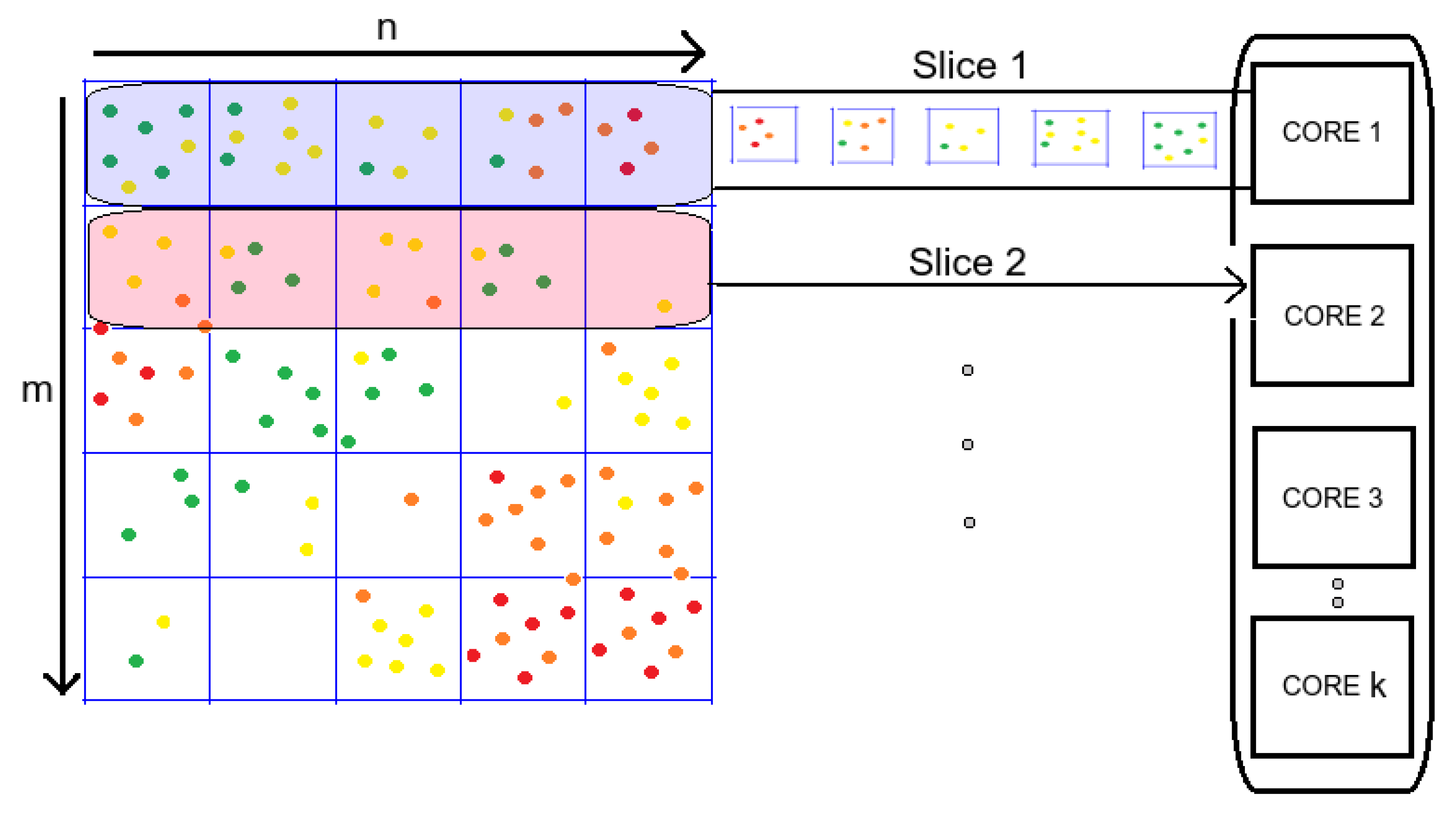
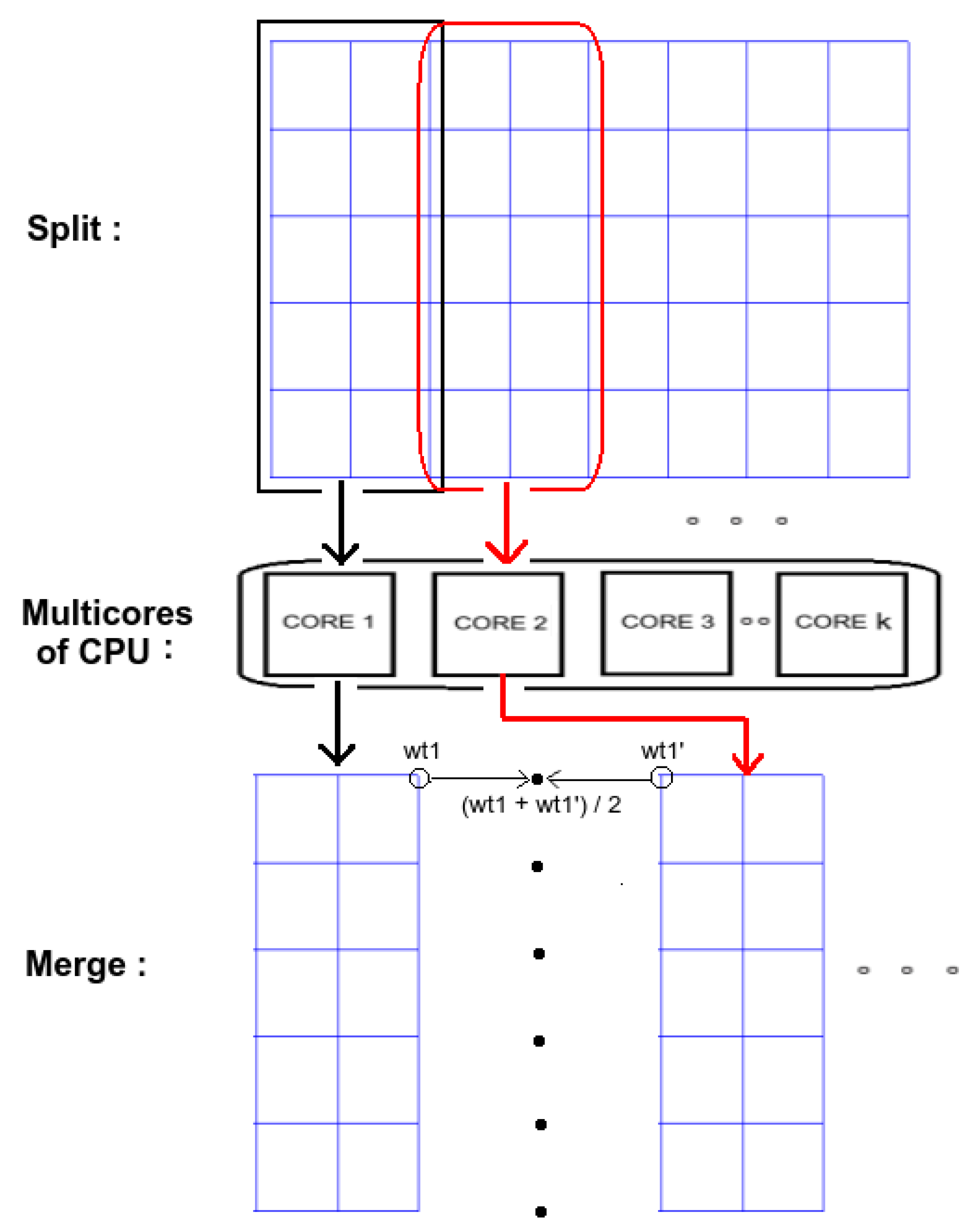
3.3. Parallel Implementation

Algorithm 1, when implemented sequentially, is extremely inefficient in terms of runtime. It takes approximately six hours to process a LiDAR point cloud of $6.94$ million points sequentially, since there can be in the worst case quadratic comparisons between points in each cell. In this section, we present a parallel implementation of the LiDAR data reduction algorithm, which is much faster than the sequential version and also highly scalable. We distribute the LiDAR data over multiple cores of the CPUs and process them in parallel using both block and cyclic assignments.

Algorithm 1 LiDAR data reduction algorithm.

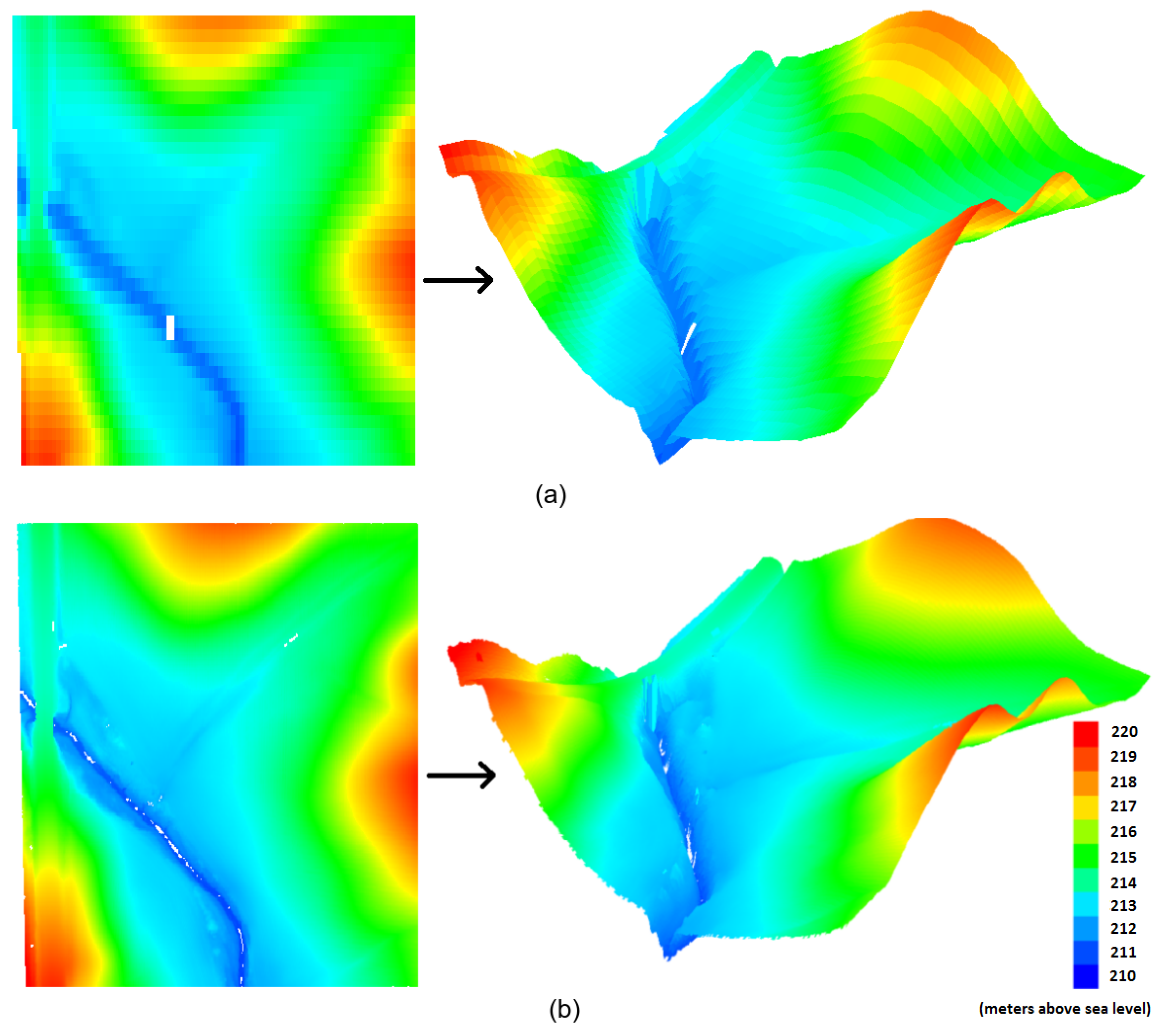
1: Input Grid of 1 sq.m. on geo-referenced LiDAR data   2: Return Reduced LiDAR data    3: Initialize: $i=0$, $cell\left[k\right]$, $p=0$, β; 4:   5: while ($cell\left[i\right]$) do 6:   Select point $p\in cell\left[i\right]$ randomly  7:   while (All points $p\in cell\left[i\right]$ are checked) do 8:       if ($p\in Slop{e}_{green}$ and $\beta \%$ of total points in $cell\left[i\right]\in Slop{e}_{green}$) then 9:             Remove all points lying in $Slop{e}_{green}$, except p;  10:             break;  11:       else if ($p\in Slop{e}_{yellow}$ and $\beta \%$ of points in $cell\left[i\right]\in Slop{e}_{yellow}$) then 12:             Remove all points lying in $Slop{e}_{yellow}$, except p;  13:             break;  14:       Select different $p\in cell\left[i\right]$ randomly;  15:   $i++$;

Consider an m rows ×n columns grid ($m,n\in \mathbb{N}$), which is overlaid on the LiDAR data as described in Section 3.2 and shown in Figure 4. For a k-core processor ($m\ge k$), we dedicate a master core, which slices the first k of m rows, and assign each one of them to each processor individually (block assignment of slices). Each of these k slices has n cells, which are processed one at a time by each core to which the corresponding slice is assigned (cyclic assignment of cells). Once every cell in all of the k slices are processed, the next k of m rows are sliced (cyclic assignment of slices) and distributed to the CPU cores, similarly as above. The results of the scalability tests using 1, 2, 4, 8 and 16 CPU cores and speed-ups are shown in Section 3.4.

3.4. Results

With the dense LiDAR data we have, consisting of $6.94$ million points, a high-accuracy (1-m vertical and horizontal accuracy) and high-resolution DEM, which covers an area $300\times 380$ sq. m. of an irregular terrain in Iowa, was generated using the IDW interpolation method (shown in Figure 5). We test our algorithm for different input values of $\beta \%$ in order to find the optimal balance between the accuracy and density of the LiDAR data. We also develop a guideline to choose the value of β for different terrains, as shown in

Table 1. Guidelines to choose the value of β for different terrains.

diff’ = max. slope - min. slope	β Range
diff $\ge 60°$	$90\le \beta \le 95$
$60>$ diff $\ge 50°$	$85\le \beta <90$
$50>$ diff $\ge 40°$	$80\le \beta <85$
diff $\le 40°$	$75\le \beta <80$

. In Figure 6a, we have shown the speed-ups and scalability test of our LiDAR data reduction algorithm for 1, 2, 4, 8 and 16 CPU cores. Using a 16-core Xeon Phi processor, we speed-up the runtime of the algorithm by $15.81$ × , i.e., from $\approx 6$ hours to $\approx 20$ minutes, for the dataset under consideration. The scalability we achieve is closer to k-fold improvement for a k-core processor ($k\ge 1$).

We observed that, compared to the DEM generated from the original, complete LiDAR dataset, there is no significant decrease in accuracy for the DEM generated from the $52\%$ reduced dataset obtained by applying our algorithm for $\beta =90\%$ to the original LiDAR dataset as input. We generate DEM from the complete LiDAR dataset, and use it as the ground truth to compare to the DEM generated from our reduced LiDAR dataset using cell by cell comparison. The Root Mean Square Error (RMSE) and standard deviation supporting the same is shown in Figure 6b. In comparison to the original DEM, the RMSE introduced in the generated DEM, when $\beta =90\%$, is only $0.14$ m. In Figure 7a, we have shown the 2D and 3D DEMs generated from the $66\%$ reduced dataset obtained by applying our algorithm for $\beta =80\%$ and in Figure 7b, the DEM generated from the $52\%$ reduced dataset obtained for $\beta =90\%$. From Figure 6b and Figure 7a, we can see that there is significant loss of accuracy in the DEM generated from the reduced dataset obtained for $\beta =80\%$ and $\beta \le 85\%$, respectively. For $\beta =80\%$, the data density is reduced by $66\%$, but there is an RMSE of $0.29$ m, which reduces the accuracy of the DEM considerably. Whereas for values of $\beta >90\%$, the percentage of data reduction is not significant.

The processing time for the DEM generation is directly proportional to the size of the LiDAR data used for its generation [24]. It takes half the time to generate DEM from the $52\%$ reduced dataset for $\beta =90\%$ compared to the original LiDAR dataset. The smaller the value of β, the lower the density of the reduced LiDAR data and the lesser is the accuracy of the DEMs generated. We need to decide the value of β based on the type of terrain; ex. based on our study, $\beta =90\%$ is optimal for terrains having a good mix of flat land, land with moderate inclination and steep slopes. It reduces the data density to half the size of the original dataset and also preserves the high accuracy of the DEMs generated. For terrains dominated by flat lands, higher β values may lead to optimal reduction of LiDAR data, whereas for terrains dominated by moderate, steep slopes and rough regions, lower values of β may be the correct choice (the value of beta is optimal when the optimal balance between accuracy and data size is maintained for DEM generations). We thus demonstrate that our LiDAR data reduction algorithm can significantly improve the processing time and the file size of DEM generations.

For certain applications, like real-time mapping of terrains using LiDAR sensors, the computational time achieved by the LiDAR data reduction filter described in Section 3, along with on-the-shelf sequential spatial interpolation algorithm is not sufficient. Hence, taking into account such applications, we develop a modified parallel IDW spatial interpolation technique, which generates better or similar quality DEMs in less computational time, compared to traditional IDW.

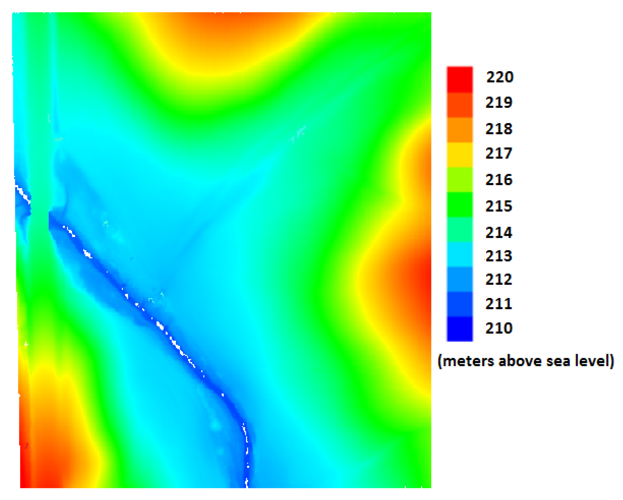
4. Spatial Interpolation

Spatial data interpolation is a crucial technique in a Geographical Information System (GIS), which computes unknown terrain height values of points, based on the known elevation values of points in the neighborhood [7]. Processing massive spatial data is a computationally-expensive and complex process, and traditional sequential algorithms cannot meet the demand for faster processing speeds along with maintaining accuracy. In this section, we describe a parallel spatial interpolation algorithm, which is a modification to QuickGrid [25] and traditional IDW. The modification takes place in the algorithm, as well as its implementation, where it exploits the multi-cores of the CPU to increase the computational speed.

4.1. Algorithm

We initialize the algorithm by overlaying a grid of k sq.m. cells ($k>0$) on the LiDAR data, while preserving spatial geo-referencing. We used $k=0.0254$ sq. m. for our simulations. Each LiDAR point has x, y and z coordinate, and we want interpolate for z-values to be assigned to each grid cell. Steps for our spatial interpolation algorithm are as follows:

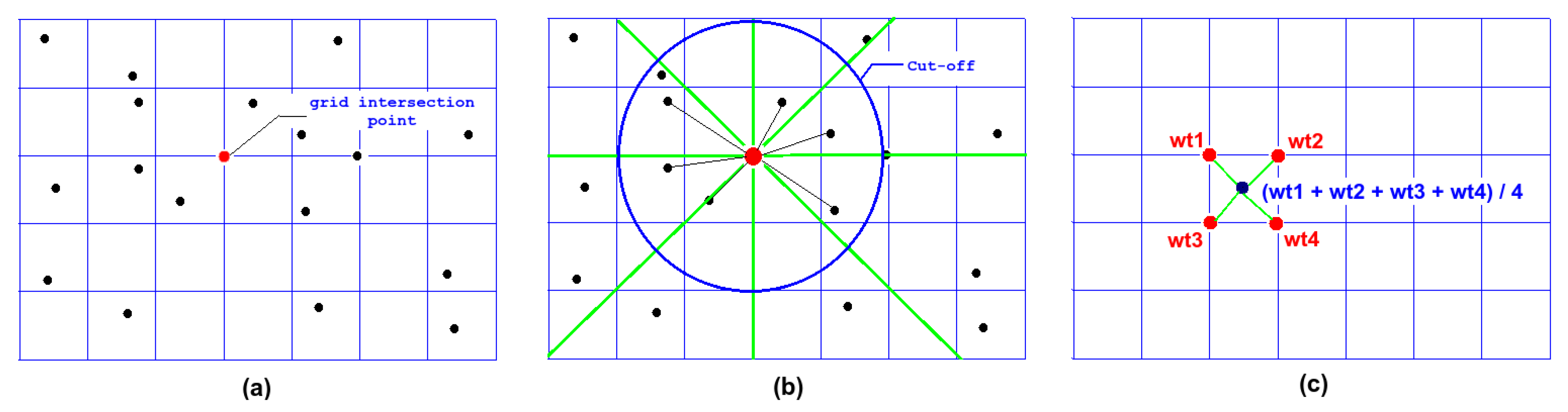
• Parse through the intersection points of each cell in the grid (shown in Figure 8a) in a left-right, top-bottom fashion.
• For each intersection point, we compute and assign a weight as follows:

  • Initially select a cut-off radius for the circle whose center is the intersection point (it is recommended to choose small cutoff radii for very dense datasets, compared to less dense datasets).
  • Then, divide the circle into eight equal sectors, and choose the closest LiDAR points in each sector, if there exist any (shown in Figure 8b). Set the grid intersection point to the average of these chosen LiDAR points weighted by 1/(distance from grid intersection)².
• After assigning weights to all of the grid intersection points, we assign each grid cell the average weight of its four surrounding grid intersection points (shown in Figure 8c).

4.2. Parallel Implementation

The sequential implementation of the algorithm described in Section 4.1 is highly inefficient in terms of processing time. Parsing over every grid cell and grid intersection points individually, multiple times, can be a computationally-expensive and time-consuming task. In this section, we design a parallel implementation for the above algorithm consisting of two phases: the split phase, where we distribute the data over multiple cores of a CPU to process it simultaneously, and the merge phase, where we merge the processed data back together.

Initially, in the split phase, we dedicate a master core, which divides the grid (along with the LiDAR data) into k equal parts, where k is the total number of CPU cores available for processing. It distributes and assigns each of the k parts of the grid to each core individually (block assignment), shown in Figure 9. Each core then simultaneously execute the algorithm mentioned in Section 4, for the part of the grid data that is assigned to it.

Once all of the cores have finished their computations, the master core initializes the merge phase, where the common grid intersection points between two grid parts are averaged and merged (shown in Figure 9), so as to get the original grid with all grid intersection points computed. Then, the master core divides the grid into k equal parts and assigns each of the k parts individually to each core, which computes and assigns to each grid cell the average weight of its surrounding four grid intersection points. Scalability tests using 1, 2, 4, 8 and 16 CPU cores and speed-ups are shown in Section 4.3.

4.3. Results

In this section, we test our spatial interpolation algorithm with fixed cut-off $1.5$ m on two different test terrains shown in Figure 5, which is our ”Dataset 1”, and in Figure 10, which is our ”Dataset 2”. Dataset 2 is $200\times 500$ m, relatively flatter with shallow valleys and less rough with the slope angle ranging from $0.07°$ to $43.8°$ when compared to Dataset 1, which is a mix of deeper valleys, steep slopes and few flat lands. Dataset 2 contains 2.1 million LiDAR points. All of the LiDAR data density reduction is done using the algorithm described in Section 3, with $\beta =90\%$. By applying our LiDAR data reduction algorithm to Dataset 1, we reduce the data density to $52\%$, and when applied to Dataset 2 for $\beta =80\%$, we reduce the data density to $71\%$. We then generate DEMs with this reduced LiDAR data, as well as the complete LiDAR dataset using traditional IDW and modified IDW.

To obtain high accuracy in our statistical analysis, we compare the elevation values of each of the LiDAR points to the corresponding elevation value of the DEMs generated, rather than checking for a few control points. This method is known as validation. RMSEs were calculated (shown in Figure 11b) to study the performance of our spatial interpolation algorithm compared to the traditional IDW algorithm, for different LiDAR data densities. From our empirical study shown in Figure 11b, we can conclude the following:

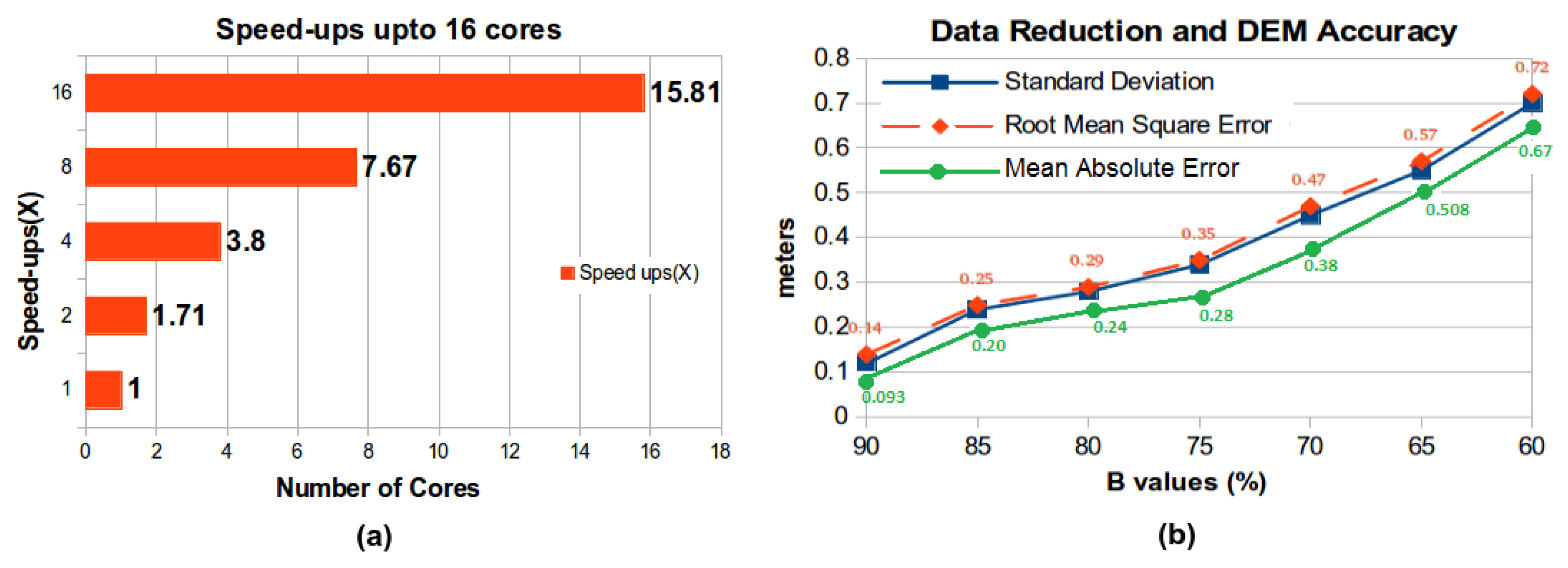
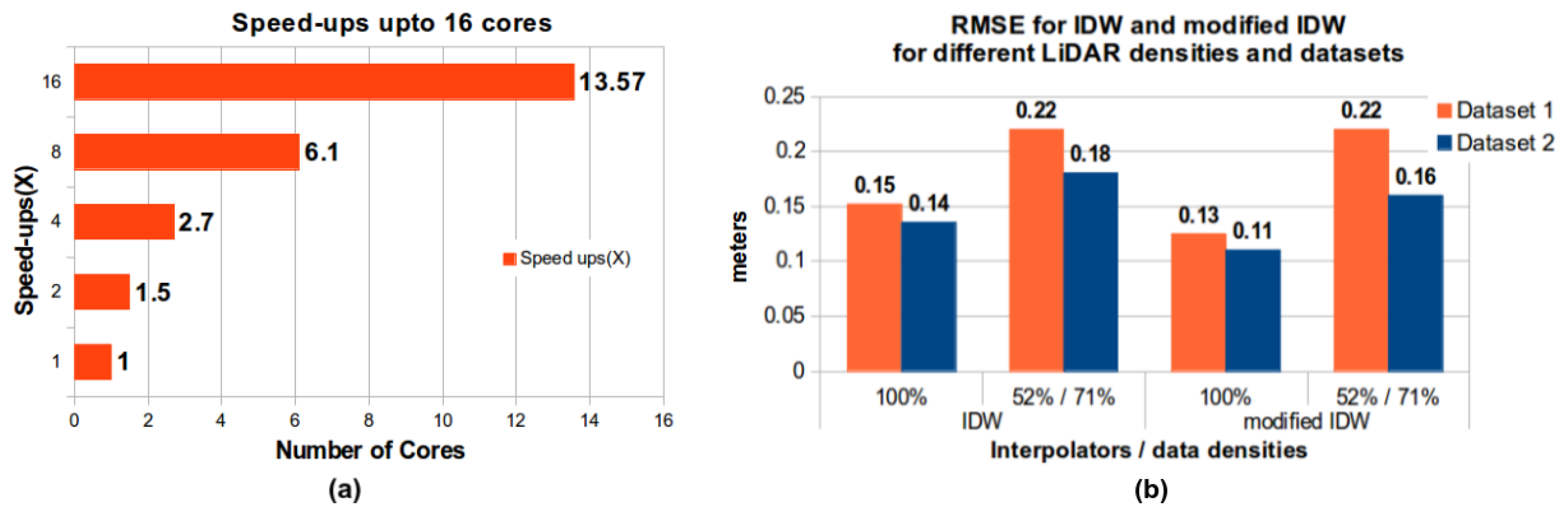
• RMSEs for both the interpolation algorithms increase with the decrease in LiDAR data density for both of the datasets.
• RMSEs for the more complex terrain, i.e., Dataset 1, are higher than Dataset 2, which is relatively flat and has shallow valleys and less roughness.
• The quality of the results obtained by modified IDW is at least as good as traditional IDW for reduced density, complex terrain (ex. 52% reduced LiDAR Dataset 1 gives an RMSE of $0.22$ m for both of the algorithms).
• The quality of the results obtained by modified IDW is better than traditional IDW for dense, complex and relatively flatter terrains.
• The time to generate DEMs using modified IDW is much less than that used by sequential traditional IDW.

As shown in Figure 11a, using a 16-core Xeon Phi processor, we speed up the running time of the algorithm by $13.5$X, i.e., 190 seconds using a single core versus 14 seconds. We implemented the LiDAR data reduction algorithm and modified IDW using C++. We use OpenMP/p-threads directives for implementing parallel versions of the above algorithms. The simulations for the LiDAR dataset is done on a system running on CentOS $6.3$, a Linux operating system based on Red Hat Linux, with 512 GB nodes, $2.9$ GHz, 16 Xeon Phi cores, high-memory node. The LiDAR point cloud, slope map and slope statistics are generated and visualized using ArcGIS, ArcMap v$10.3$. The IDW algorithm is used to generate DEMs for reduced LiDAR data (not our new spatial interpolation algorithm). We use the QuickGrid tool to visualize DEM’s generated by our spatial interpolation algorithm, as well as the data reduction algorithm. All of the plots are done using Gnuplot and LibreDraw. All of the results obtained are the average of five runs.

5. Conclusions and Future Work

It is observed that not all LiDAR data contribute effectively to the accurate generation of DEMs. It is important to identify points representing the specific features of the terrain that contain more significant information, compared to other points [9,11]. While designing our LiDAR data reduction algorithm, we mainly take into consideration the slope of the terrain, to remove less important points and keep critical points. Terrain slopes highlight changes in the terrain surfaces, which provide elevation information of a point, and they also showcase information about their surroundings. Significant changes in slopes of the terrain indicate points with more critical information, compared to other points [7]. Thus, using our LiDAR data reduction algorithm, we decrease the number of data points required for DEM generation, along with maintaining high accuracy. Results show that our parallel implementation of this algorithm is highly scalable and efficient in terms of processing times.

The modified IDW spatial interpolation technique, which we present in this paper, achieves results that are at least as good as traditional IDW for reduced density, complex terrain and better than traditional IDW for dense, complex and relatively flatter terrains. It also achieves good scalability and takes much less time to generate DEMs compared to traditional IDW.

For testing our spatial interpolation algorithm, we set the cut-off to $1.5$ m for the entire terrain. However, larger cut-offs for flat parts of the terrain and smaller cut-offs for rough and complex parts are ideal. Therefore, a technique that varies the cut-offs of our algorithm, based on the topographical features of the terrain, would be interesting to see. To achieve higher speed-ups from more cores, GPU-based algorithms can be developed along the same lines as our multicore algorithms. Furthermore, our parallel IDW algorithm can also be integrated with our data reduction algorithm and used as a core subroutine in some streaming-based applications.

References

1. Habib, A.; Ghanma, M.; Morgan, M.; Al-Ruzouq, R. Photogrammetric and LiDAR data registration using linear features. Photogramm. Eng. Remote Sens. 2005, 71, 699–707. [Google Scholar] [CrossRef]
2. Sithole, G.; Vosselman, G. The Full Report: ISPRS Comparision of Filters. Available online: http://www.itc.nl /isprswgIII-3/filtertest/ (accessed on 30 April 2016).
3. Hodgson, M.E.; Bresnahan, P. Accuracy of airborne LiDAR-derived elevation. Photogramm. Eng. Remote Sens. 2004, 70, 331–339. [Google Scholar] [CrossRef]
4. El-Sheimy, N.; Valeo, C.; Habib, A. Digital Terrain Modeling: Acquisition, Manipulation, and Applications; Artech House: London, UK, 2005. [Google Scholar]
5. Ramirez, J.R. A new approach to relief representation. Surv. Land Inf. Sci. 2006, 66, 19–25. [Google Scholar]
6. Burrough, P.A.; McDonnell, R.A. Principles of Geographical Information Systems; Oxford University Press: New York, NY, USA, 2011. [Google Scholar]
7. Li, Z.; Zhu, C.; Gold, C. Digital Terrain Modeling: Principles and Methodology; CRC Press: Boca Raton, FL, USA, 2004. [Google Scholar]
8. Bonham-Carter, G.F. Geographic Information Systems for Geoscientists: Modelling with GIS; Elsevier: Amsterdam, the Netherlands, 2014. [Google Scholar]
9. Chou, Y.-H.; Liu, P.-S.; Dezzani, R.J. Terrain complexity and reduction of topographic data. J. Geogr. Syst. 1999, 1, 179–198. [Google Scholar] [CrossRef]
10. Anderson, E.S.; Thompson, J.A.; Austin, R.E. LiDAR density and linear interpolator effects on elevation estimates. Int. J. Remote Sens. 2005, 26, 3889–3900. [Google Scholar] [CrossRef]
11. Liu, X.; Zhang, Z. LiDAR data reduction for efficient and high quality DEM generation. Int. Arch. Photogramm. Remote Sens. Spat. Inf. Sci. 2008, 37, 173–178. [Google Scholar]
12. Oryspayev, D.; Sugumaran, R.; DeGroote, J.; Gray, P. LiDAR data reduction using vertex decimation and processing with GPGPU and multicore CPU technology. Comput. Geosci. 2012, 43, 118–125. [Google Scholar] [CrossRef]
13. Hegeman, J.W.; Sardeshmukh, V.B.; Sugumaran, R.; Armstrong, M.P. Distributed LiDAR data processing in a high-memory cloud-computing environment. Ann. GIS 2014, 20, 255–264. [Google Scholar] [CrossRef]
14. Kobler, A.; Pfeifer, N.; Ogrinc, P.; Todorovski, L.; Oštir, K.; Džeroski, S. Repetitive interpolation: A robust algorithm for DTM generation from Aerial Laser Scanner Data in forested terrain. Remote Sens. Environ. 2007, 108, 9–23. [Google Scholar] [CrossRef]
15. ZakÅ¡ek, K.; Pfeifer, N.; IAPÅ, Z.S. An Improved Morphological Filter for Selecting Relief Points from a LiDAR Point Cloud in Steep Areas with Dense Vegetation; Institute of Anthropological and Spatial Studies, Scientific Research Centre of the Slovenian Academy of Sciences and Arts: Luubljana, Slovenia; Institute of Geography, Innsbruck University: Innsbruck, Austria, 2006. [Google Scholar]
16. Kraus, K.; Otepka, J. DTM Modelling and Visualization—The Scop Approach. In Proceedings of Photogrammetric Week 05, Heidelberg, Germany; 2005; pp. 241–252. [Google Scholar]
17. Liu, X.; Zhang, Z.; Peterson, J.; Chandra, S. Lidar-derived high quality ground control information and DEM for image orthorectification. GeoInformatica 2007, 11, 37–53. [Google Scholar] [CrossRef] [Green Version]
18. Zimmerman, D.; Pavlik, C.; Ruggles, A.; Armstrong, M.P. An experimental comparison of ordinary and universal kriging and inverse distance weighting. Math. Geol. 1999, 31, 375–390. [Google Scholar] [CrossRef]
19. Liu, X.; Zhang, Z.; Peterson, J. Evaluation of the performance of DEM interpolation algorithms for LiDAR data. In Proceedings of the Surveying and Spatial Sciences Institute Biennial International Conference (SSC 2009), Adelaide, Australia, 28 September–2 October 2009; pp. 771–779.
20. Fisher, P.F.; Tate, N.J. Causes and consequences of error in digital elevation models. Prog. Phys. Geogr. 2006, 30, 467–489. [Google Scholar] [CrossRef]
21. Podobnikar, T. Suitable DEM for required application. In Proceedings of the 4th International Symposium on Digital Earth, Tokyo, Japan, 28–31 March 2005.
22. Ali, T.A. On the selection of an interpolation method for creating a terrain model (TM) from LiDAR data. In Proceedings of the American Congress on Surveying and Mapping (ACSM) Conference, Nashville, TN, USA; 2004. [Google Scholar]
23. The National Map–Elevation. Available online: http://ned.usgs.gov/ (accessed on 30 April 2016).
24. Liu, X.; Zhang, Z.; Peterson, J.; Chandra, S. The effect of LiDAR data density on DEM accuracy. In Proceedings of the International Congress on Modelling and Simulation (MODSIM07), Christchurch, New Zealand, 10–13 December 2007; pp. 1363–1369.
25. Coulthard, J. Quikgrid: 3-D Rendering of a Surface Represented by Scattered Data Points. Available online: http://www.galiander.ca/quikgrid/ (accessed on 30 April 2016).
Figure 1. (a) Imagery of the study area and (b) 2D LiDAR point cloud of the study area, which is colored based on the variations in elevation.
Ijgi 05 00097 g001
Figure 2. (a) Statistical analysis of elevation data for the terrain; (b) slope map consisting of four slope ranges.
Ijgi 05 00097 g002
Figure 3. Data reduction algorithm: grid overlayed on processed LiDAR data.
Ijgi 05 00097 g003
Figure 4. Parallel implementation of the data reduction algorithm.
Ijgi 05 00097 g004
Figure 5. DEM generated for the original dataset having 6 . 94 million LiDAR points.
Ijgi 05 00097 g005
Figure 6. (a) Parallel speed-ups for the LiDAR data reduction algorithm; (b) data reduction and DEM accuracy.
Ijgi 05 00097 g006
Figure 7. (a) β = 80 % , reduced dataset comprised of 2 . 2 million points; (b) β = 90 % , reduced dataset containing 3 . 1 million points.
Ijgi 05 00097 g007
Figure 8. (a) Grid of k sq. m. ( k > 0 ) overlaid on the LiDAR data; (b) selecting cut-off radii and assigning weights to grid intersections; (c) assigning weights to each grid cell.
Ijgi 05 00097 g008
Figure 9. Parallel split and merge phases of our spatial interpolation algorithm.
Ijgi 05 00097 g009
Figure 10. (a) Imagery of the study area for Dataset 2; (b) elevation map of Dataset 2 showing terrain with less roughness, shallow valleys and flat regions.
Ijgi 05 00097 g010
Figure 11. (a) Parallel speed-ups for our spatial algorithm; (b) RMSE for IDW and modified IDW at different LiDAR density levels for two datasets using the validation method.
Ijgi 05 00097 g011