
Evaluation of Deterministic and Complex Analytical Hierarchy Process Methods for Agricultural Land Suitability Analysis in a Changing Climate

Abstract
:1. Introduction
2. Methods
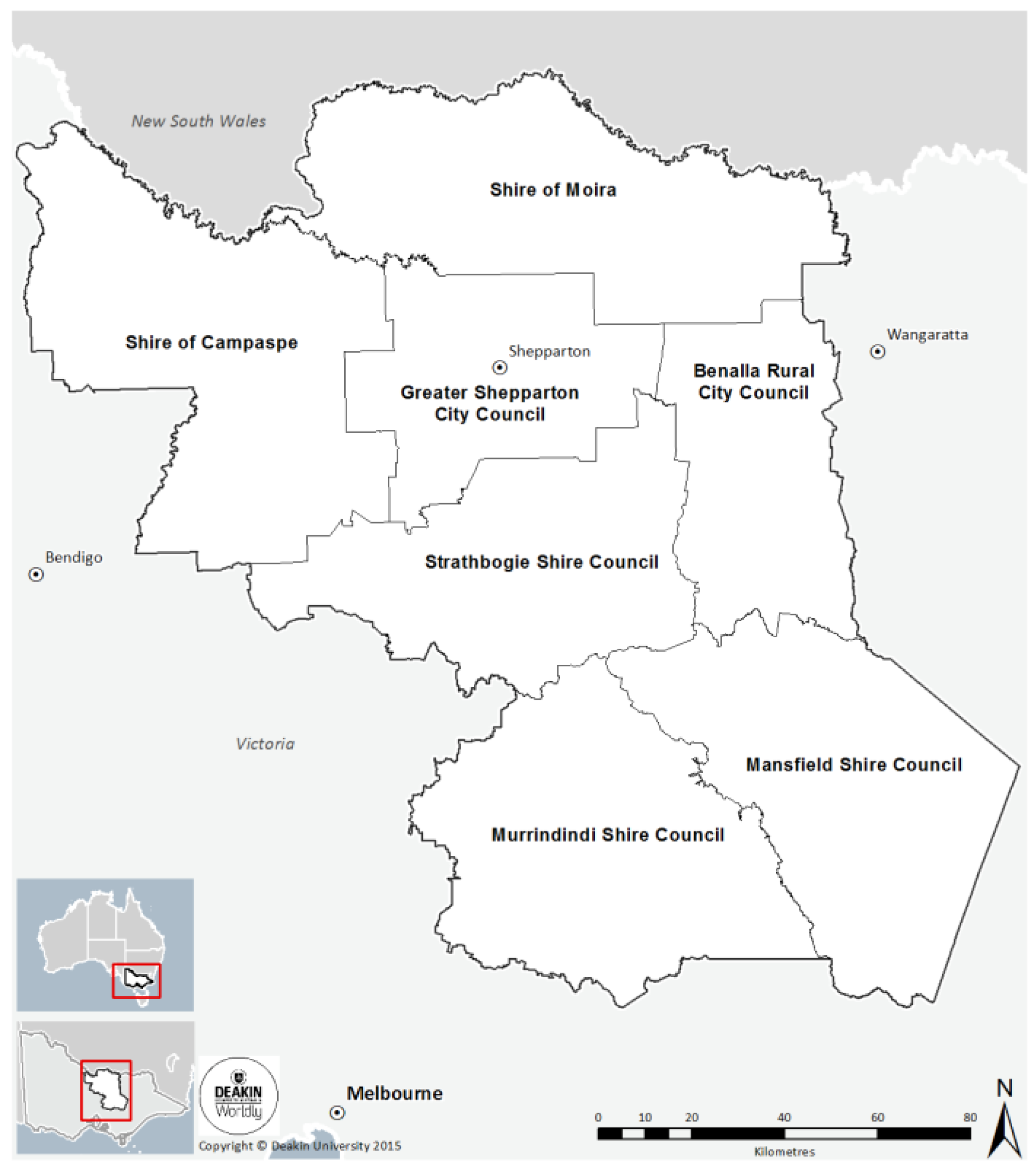
2.1. Study Region
2.2. Land Suitability Analysis
2.3. Analytical Hierarchy Process
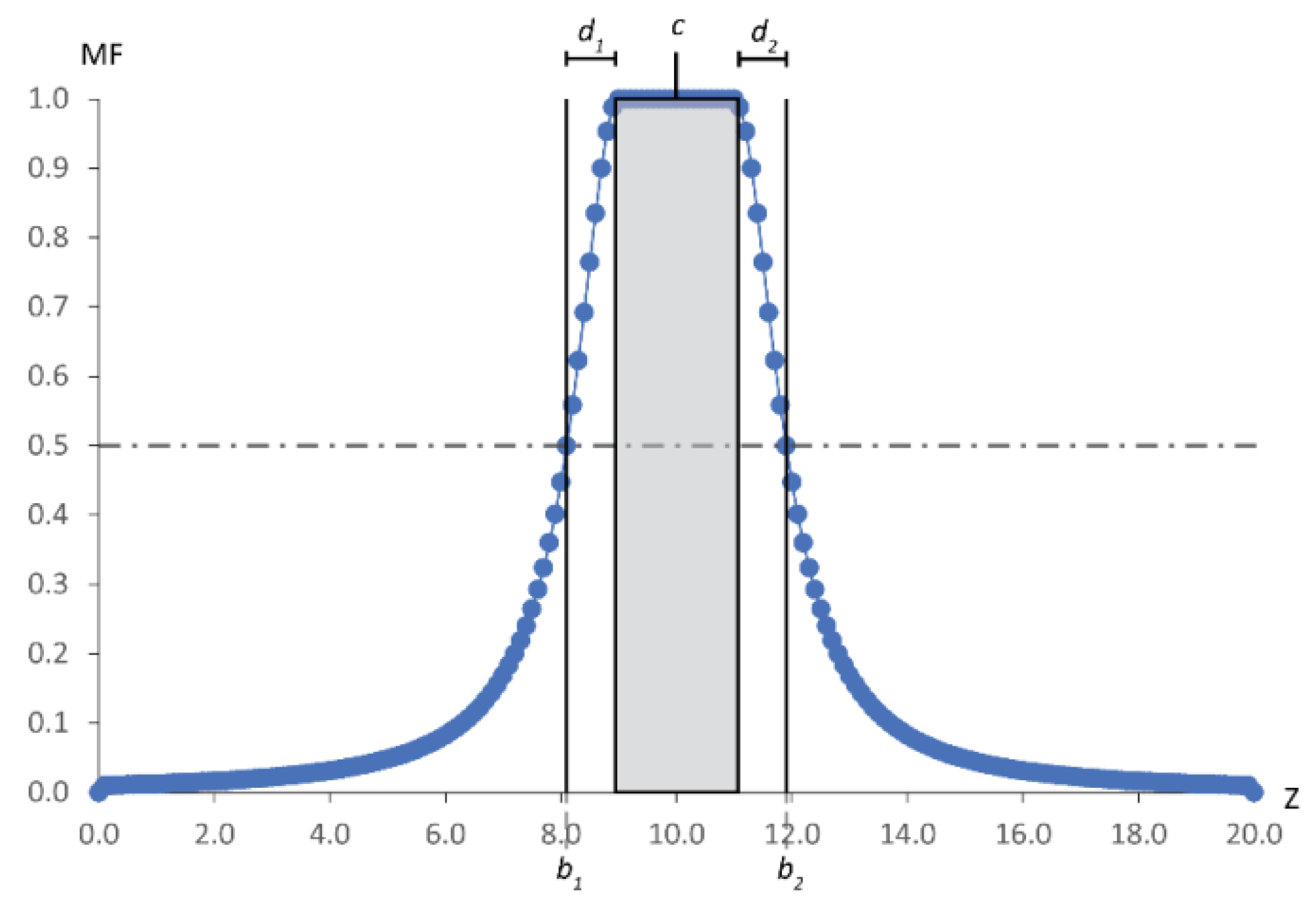
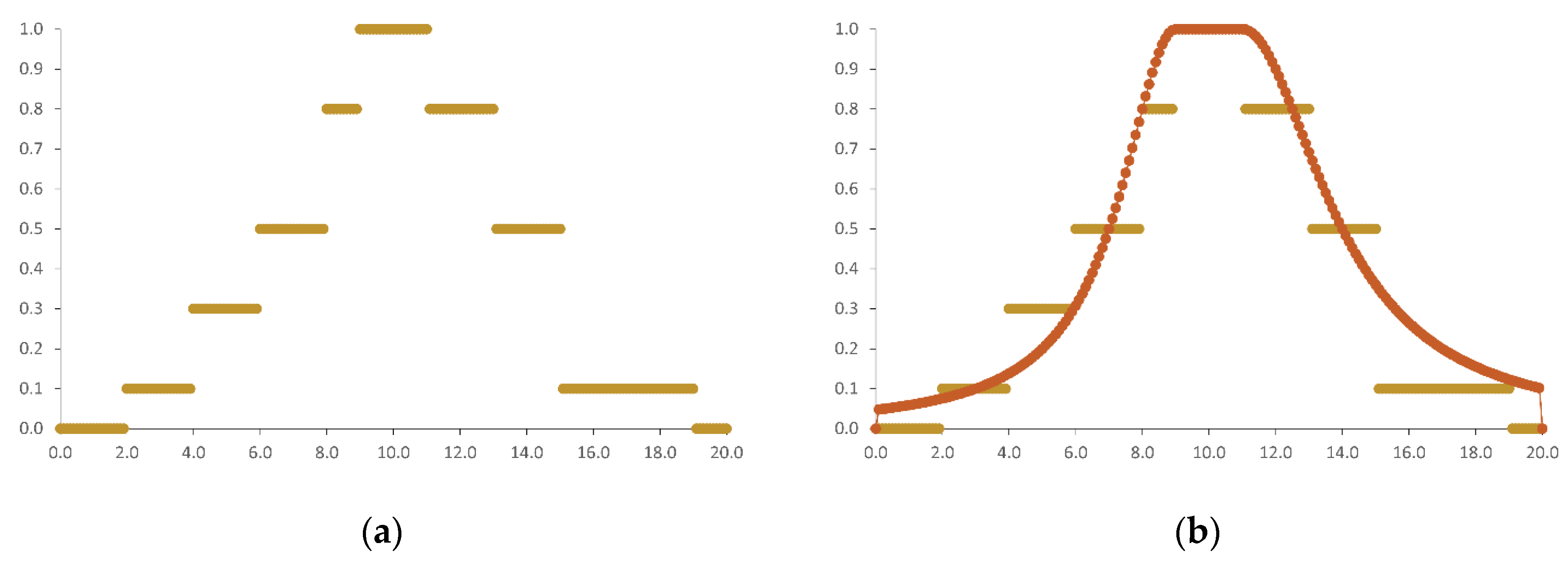
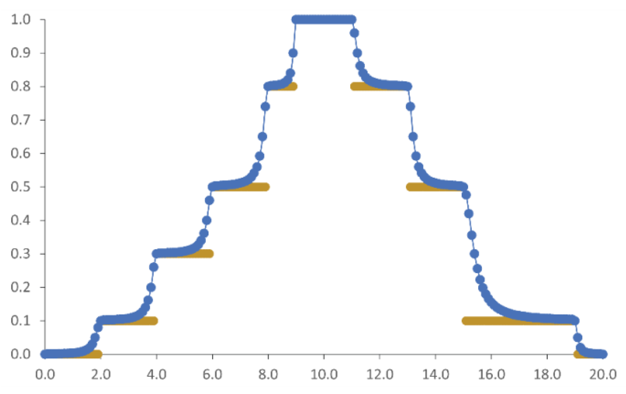
2.4. Fuzzy Set Modelling
2.5. Model Inputs and Application
3. Results
3.1. Standard AHP Outputs
3.2. Fuzzy Set Modelling Outputs
3.3. Output Comparisons
4. Results Discussion
5. Concluding Comments
Acknowledgments
Author Contributions
Conflicts of Interest
References
- Olesen, J.E.; Bindi, M. Consequences of climate change for European agricultural productivity, land use and policy. Eur. J. Agron. 2002, 16, 239–262. [Google Scholar] [CrossRef]
- Keshavarzi, A.; Sarmadian, F.; Heidari, A.; Omid, M. Land suitability evaluation using fuzzy continuous classification (A case study: Ziaran region). Mod. Appl. Sci. 2010, 4, 72. [Google Scholar] [CrossRef]
- FAO. A Framework for Land Evaluation; FAO Soils Bulletin; Food and Agriculture Organisation of the United Nations: Rome, Italy, 1976. [Google Scholar]
- Wang, F.; Brent Hall, G.; Subaryono. Fuzzy information representation and processing in conventional GIS software: Database design and application. Int. J. Geogr. Inf. Syst. 1990, 4, 261–283. [Google Scholar] [CrossRef]
- Nisar Ahamed, T.R.; Gopal Rao, K.; Murthy, J.S.R. GIS-based fuzzy membership model for crop-land suitability analysis. Agric. Syst. 2000, 63, 75–95. [Google Scholar] [CrossRef]
- Carver, S.J. Integrating multi-criteria evaluation with geographical information systems. Int. J. Geogr. Inf. Syst. 1991, 5, 321–339. [Google Scholar] [CrossRef]
- Jankowski, P.; Richard, L. Integration of GIS-based suitability analysis and multicriteria evaluation in a spatial decision support system for route selection. Environ. Plan. B Plan. Des. 1994, 21, 323–340. [Google Scholar] [CrossRef]
- Hossain, H.; Sposito, V.; Evans, C. Sustainable land resource assessment in regional and urban systems. Appl. GIS 2006, 2, 24.1–24.21. [Google Scholar] [CrossRef]
- Dujmovic, J.J.; de Tré, G.; Dragicevic, S. Comparison of multicriteria methods for land-use suitability assessment. In Proceedings of the Joint 2009 International Fuzzy Systems Association World Congress and 2009 European Society of Fuzzy Logic and Technology Conference IFSA/EUSFLAT, Lisbon, Portugal, 20–24 July 2009.
- McHarg, I.L. Design with Nature; Published for the American Museum of Natural History; Natural History Press: Garden City, NY, USA, 1969. [Google Scholar]
- Saaty, T.L. The analytic Hierarchy Process: Planning, Priority Setting, Resource Allocation; McGraw-Hill International Book Co.: New York, NY, USA; London, UK, 1980. [Google Scholar]
- Saaty, T.L. Fundamentals of Decision Making, and Prority Theory: With the Analytic Hierarchy Process, 1st ed.; Analytic Hierarchy Process Series; RWS Publications: Pittsburgh, PA, USA, 1994. [Google Scholar]
- Saaty, T.L. Decision Making for Leaders: The Analytical Hierarchy Process for Decisions in a Complex World, 3rd ed.; RWS Publications: Pittsburgh, PA, USA, 1995. [Google Scholar]
- Mikhailov, L. Deriving priorities from fuzzy pairwise comparison judgements. Fuzzy Sets Syst. 2003, 134, 365–385. [Google Scholar] [CrossRef]
- Elaalem, M. A Comparison of Parametric and Fuzzy Multi-Criteria Methods for Evaluating Land Suitability for Olive in Jeffara Plain of Libya. APCBEE Procedia 2013, 5, 405–409. [Google Scholar] [CrossRef]
- Zadeh, L.A. Fuzzy sets. Inf. Control 1965, 8, 338–353. [Google Scholar] [CrossRef]
- Zadeh, L.A. Fuzzy Sets and Their Applications to Cognitive and Decision Processes; Academic Press: New York, NY, USA, 1975. [Google Scholar]
- Burrough, P.; MacMillan, R.; Deursen, W.V. Fuzzy classification methods for determining land suitability from soil profile observations and topography. J. Soil Sci. 1992, 43, 193–210. [Google Scholar] [CrossRef]
- Liu, Y.; Jiao, L.; Liu, Y.; He, J. A self-adapting fuzzy inference system for the evaluation of agricultural land. Environ. Model. Softw. 2013, 40, 226–234. [Google Scholar] [CrossRef]
- Burrough, P.A.; McDonnell, R.A.; Lloyd, C.D. Principles of Geographical Information Systems, 3rd ed.; Oxford University Press: Oxford, UK, 2015. [Google Scholar]
- Sicat, R.S.; Carranza, E.J.M.; Nidumolu, U.B. Fuzzy modeling of farmers’ knowledge for land suitability classification. Agric. Syst. 2005, 83, 49–75. [Google Scholar] [CrossRef]
- Reshmidevi, T.V.; Eldho, T.I.; Jana, R. A GIS-integrated fuzzy rule-based inference system for land suitability evaluation in agricultural watersheds. Agric. Syst. 2009, 101, 101–109. [Google Scholar] [CrossRef]
- Ceballos-Silva, A.; Lopez-Blanco, J. Delineation of suitable areas for crops using a Multi-Criteria Evaluation approach and land use/cover mapping: A case study in Central Mexico. Agric. Syst. 2003, 77, 117–136. [Google Scholar] [CrossRef]
- Voogd, H. Multicriteria Evaluation for Urban and Regional Planning; Pion.: London, UK, 1983; Volume 14, p. 367. [Google Scholar]
- Malczewski, J. GIS-based land-use suitability analysis: A critical overview. Prog. Plan. 2004, 62, 3–65. [Google Scholar] [CrossRef]
- Chen, Y.; Yu, J.; Khan, S. The spatial framework for weight sensitivity analysis in AHP-based multi-criteria decision making. Environ. Model. Softw. 2013, 48, 129–140. [Google Scholar] [CrossRef]
- Zhang, J.; Su, Y.; Wu, J.; Liang, H. GIS based land suitability assessment for tobacco production using AHP and fuzzy set in Shandong province of China. Comput. Electron. Agric. 2015, 114, 202–211. [Google Scholar] [CrossRef]
- Sposito, V.A.; Benke, K.; Pelizaro, C.; Wyatt, R. Adaptation to climate change in regional australia: A decision-making framework for modelling policy for rural production. Geogr. Compass 2010, 4, 335–354. [Google Scholar] [CrossRef]
- Houshyar, E.; SheikhDavoodi, M.J.; Almassi, M.; Bahrami, H.; Azadi, H.; Omidi, M.; Sayyad, G.; Witlox, F. Silage corn production in conventional and conservation tillage systems. Part I: Sustainability analysis using combination of GIS/AHP and multi-fuzzy modeling. Ecol. Ind. 2014, 39, 102–114. [Google Scholar] [CrossRef]
- Zimmermann, H.J.; Zadeh, L.A.; Gaines, B.R. Fuzzy Sets and Decision Analysis; TIMS studies in the Management Sciences; North-Holland Distributors; Elsevier Science: Amsterdam, The Netherlands; New York, NY, USA, 1984; p. 522. [Google Scholar]
- Gordon, H.B.; Collier, M.; Dix, M.; Rotstayn, L.; Kowalczyk, E.; Hirst, T.; Watterson, I. The CSIRO Mk3. 5 Climate Model; CAWCR: Melbourne, Australia, 2010. [Google Scholar]
- Nakicenovic, N.; Alcamo, J.; Davis, G.; de Vries, B.; Fenhann, J.; Gaffin, S.; Gregory, K.; Grubler, A.; Jung, T.A.; Kram, T. Special Report on Emissions Scenarios: A Special Report of Working Group III of the Intergovernmental Panel on Climate Change; Pacific Northwest National Laboratory, Environmental Molecular Sciences Laboratory (US): Richland, WA, USA, 2000.


| Intensity Rating | Definition |
|---|---|
| 1 | X is of equal importance to Y |
| 3 | X is slightly more influential than Y |
| 5 | X is more influential than Y |
| 7 | X is highly more influential than Y |
| 9 | X is definitely more influential than Y |
| Criteria | Weight (%) | Suitability Class | Index Value | Membership Function | |||||||
|---|---|---|---|---|---|---|---|---|---|---|---|
| 1st | 2nd | 3rd | 1st | 2nd | 3rd | High | Low | High | Low | Equations | Curve Behaviour |
| Landscape | 5 | ||||||||||
| Slope | 90 | <1.8° | >18° | 1.0 | −1.0 (Perm) | (3) | Negative | ||||
| Aspect | 10 | N, E, W | S | 1.0 | 0.6 | (1)–(3) | Full | ||||
| Soil | 30 | ||||||||||
| pH | 10 | 5.8–7.0 | <4.0 and >8.5 | 1.0 | −1.0 (Temp) | (1)–(3) | Full | ||||
| Sodicity | 10 | Not Sodic | Sodic | 1.0 | 0.6 | n.a. | n.a. | ||||
| Useable Depth | 25 | >45 cm | <10 cm | 1.0 | −1.0 (Perm) | (1) | Positive | ||||
| Texture | 25 | CL, L, LC, SL | S, HC | 1.0 | 0.1 | n.a. | n.a. | ||||
| Drainage | 10 | Well, Moderate | Very Poor | 1.0 | 0.1 | n.a. | n.a. | ||||
| ECe | 20 | Very Low | Very High | 1.0 | −1.0 (Perm) | n.a. | n.a. | ||||
| Climate | 65 | ||||||||||
| Temperature | 45 | ||||||||||
| Minimum Temperature | 50 | ||||||||||
| September–October | 70 | 4–20 °C | <−2 °C | 1.0 | 0.0 | (1)–(3) | Full | ||||
| November–March | 30 | 15–20 °C | <10 °C, >25 °C | 1.0 | 0.0 | (1)–(3) | Full | ||||
| Maximum Temperature | 50 | ||||||||||
| September–October | 70 | 4–20 °C | <−2 °C, >25 °C | 1.0 | 0.0 | (1)–(3) | Full | ||||
| November–March | 30 | <25 °C | >32 °C | 1.0 | 0.0 | (3) | Negative | ||||
| Wind | 5 | <5 km/h | >30 km/h | 1.0 | 0.5 | (3) | Negative | ||||
| Chill Units | 5 | >500 CU | <300 CU | 1.0 | 0.0 | (1) | Positive | ||||
| Water Availability | 45 | ||||||||||
| June–August | 40 | 50–120 mm | <35 mm, >120 mm | 1.0 | 0.0 | (1)–(3) | Full | ||||
| September–October | 10 | <40 mm | >120 mm | 1.0 | 0.0 | (3) | Negative | ||||
| November–January | 30 | 20–45 mm | >135 mm | 1.0 | 0.0 | (1)–(3) | Full | ||||
| May | 20 | 20–150 mm | >200 mm | 1.0 | 0.0 | (1)–(3) | Full | ||||
| Suitability Index Value | Standard | Fitted | Nested | |||
|---|---|---|---|---|---|---|
| Normal | 2050 | Normal | 2050 | Normal | 2050 | |
| Hectares (ha) | ||||||
| TNS 1 | 8045 (0.3%) | 8045 (0.3%) | 8045 (0.3%) | 8045 (0.3%) | 8045 (0.3%) | 8045 (0.3%) |
| PNS 2 | 320,632 (13.1%) | 320,632 (13.1%) | 178,508 (7.3%) | 178,508 (7.3%) | 178,508 (7.3%) | 178,508 (7.3%) |
| 60% | 3 (>0.1%) | - | - | - | - | - |
| 70% | 29,674 (1.2%) | 489,530 (20.0%) | 3513 (0.1%) | 24,129 (1.0%) | 16,713 (0.7%) | 67,159 (2.8%) |
| 80% | 340,934 (14.0%) | 487,400 (20.0%) | 277,150 (11.4%) | 533,325 (21.8%) | 226,459 (9.3%) | 665,944 (27.3%) |
| 90% | 1,431,712 (58.6%) | 1,008,898 (41.3%) | 1,655,614 (67.8%) | 1,576,833 (64.6%) | 1,999,149 (81.9%) | 1,508,904 (61.8%) |
| 100% | 310,643 (12.7%) | 127,138 (5.2%) | 318,813 (13.1%) | 120,803 (4.9%) | 12,769 (0.5%) | 13,083 (0.5%) |
© 2016 by the authors; licensee MDPI, Basel, Switzerland. This article is an open access article distributed under the terms and conditions of the Creative Commons Attribution (CC-BY) license (http://creativecommons.org/licenses/by/4.0/).
Share and Cite
Romeijn, H.; Faggian, R.; Diogo, V.; Sposito, V. Evaluation of Deterministic and Complex Analytical Hierarchy Process Methods for Agricultural Land Suitability Analysis in a Changing Climate. ISPRS Int. J. Geo-Inf. 2016, 5, 99. https://0-doi-org.brum.beds.ac.uk/10.3390/ijgi5060099
Romeijn H, Faggian R, Diogo V, Sposito V. Evaluation of Deterministic and Complex Analytical Hierarchy Process Methods for Agricultural Land Suitability Analysis in a Changing Climate. ISPRS International Journal of Geo-Information. 2016; 5(6):99. https://0-doi-org.brum.beds.ac.uk/10.3390/ijgi5060099
Chicago/Turabian StyleRomeijn, Harmen, Robert Faggian, Vasco Diogo, and Victor Sposito. 2016. "Evaluation of Deterministic and Complex Analytical Hierarchy Process Methods for Agricultural Land Suitability Analysis in a Changing Climate" ISPRS International Journal of Geo-Information 5, no. 6: 99. https://0-doi-org.brum.beds.ac.uk/10.3390/ijgi5060099