Exploring the Influence of Neighborhood Characteristics on Burglary Risks: A Bayesian Random Effects Modeling Approach

Abstract

A Bayesian random effects modeling approach was used to examine the influence of neighborhood characteristics on burglary risks in Jianghan District, Wuhan, China. This random effects model is essentially spatial; a spatially structured random effects term and an unstructured random effects term are added to the traditional non-spatial Poisson regression model. Based on social disorganization and routine activity theories, five covariates extracted from the available data at the neighborhood level were used in the modeling. Three regression models were fitted and compared by the deviance information criterion to identify which model best fit our data. A comparison of the results from the three models indicates that the Bayesian random effects model is superior to the non-spatial models in fitting the data and estimating regression coefficients. Our results also show that neighborhoods with above average bar density and department store density have higher burglary risks. Neighborhood-specific burglary risks and posterior probabilities of neighborhoods having a burglary risk greater than 1.0 were mapped, indicating the neighborhoods that should warrant more attention and be prioritized for crime intervention and reduction. Implications and limitations of the study are discussed in our concluding section.

1. Introduction

Researchers have long been interested in the relationship between crime and place [1]. Traditional criminological interest in place is mainly focused on macro levels of geography such as countries [2,3], states [4], counties [5] and cities [6,7]. Recently, there has been a growing interest in crime at small-area scales, which include blocks [8], neighborhoods [9], street segments [10], face blocks [11] and other defined small-area units of analysis. Studies of crime at small scales have great practical benefits and are of tremendous value to law enforcement. In addition to providing relatively precise and easier targets than big units of analysis for police department to oversee, they also provide a more detailed and robust understanding of the complex relationship between crime and place, contributing to scientific crime prevention and control.

Traditional non-spatial regression approaches assume that crime counts or crime rates are independent and identically distributed. This hypothesis ignores spatial dependence between crime counts and crime rates, especially at small-area scales. In addition, some covariates, for example income and unemployment rate, are also likely to be spatially auto-correlated. In ecological studies of crime, if spatial dependence is present but neglected, standard errors of regression coefficients may be underestimated, inducing biased and inefficient inferences [12]. For example, covariates may be incorrectly identified as significant. Thus, non-spatial models are inappropriate for crime analysis at small-area levels.

To overcome the shortcomings of non-spatial models in criminological studies, most researchers adopt a spatial lag model, spatial error model or some other frequentist statistical models from a spatial perspective [13,14,15,16]. The spatial lag model and spatial error model [17] are unsuitable for modeling discrete variables because they both require the dependent variable to be continuous and follow a normal distribution. If the discrete crime count is the response variable, these models would be inappropriate. Additionally, complex spatial models, for example the spatial logistic model and the spatial probit model that account for spatial autocorrelation, are difficult to fit under frequency-based methods.

Bayesian statistics, as the other school of thought of statistics, has also been applied to spatial analysis. In contrast to frequentist statistics, Bayesian statistics treats all unknown parameters as random variables with probability distributions. It is based on the principle that prior knowledge and data are combined together to derive posterior estimates for parameters of interest. Bayesian approaches to modeling spatial data have received growing attention since the 1990s. This owes much to improvements of Markov chain Monte Carlo (MCMC) methods that make it possible to fit most Bayesian models, the availability of software such as WinBUGS to implement MCMC [18,19] and the rapid evolution of powerful computers. Bayesian approaches combined with MCMC are appropriate for exploration of complex (spatial) models that would otherwise be difficult to fit with frequentist statistics. Although Bayesian statistics have been found to be fashionable in science and widely used in epidemiology and environmental health problems, especially disease mapping and modeling [20,21,22,23], their application to crime analysis is still rare. However, researchers are increasingly aware of the advantages of Bayesian spatial modeling in small-area crime analysis. The past few years have seen a small but growing body of literature applying Bayesian spatial approaches in crime researches [24,25,26,27,28,29,30,31,32,33,34,35]. For example, the relationship between alcohol outlets and domestic violence (intimate partner violence and child abuse) has been illustrated in a couple of ecological studies [25,29]. Other neighborhood-level characteristics have also been linked to domestic violence [32,35]. Several recent papers have also examined contextual influences on juvenile offenders and property crime using a Bayesian Spatial modeling approach [30,31,33]. Bayesian spatial models could be used not only to analyze continuous variables such as crime rates, but also to model discrete variables such as raw crime counts.

The primary goal of our research is to explore the influence of neighborhood characteristics on burglary risks by adopting a Bayesian random effects modeling approach. This modeling approach is seldom applied to the study of burglary risks. The Bayesian random effects models extend generalized linear models by including one or more random effects terms. These random effects contribute to stabilizing risk estimates for small areas by borrowing strength from adjacent areas, thus overcoming unstable estimates due to the small number problem [21,36]. This method allows more flexibility when specifying the spatial autocorrelation that often exists in crime data, especially at small-area scales. In addition, random effects modeling is also appropriate when, due to data limitations, some covariates that themselves have a spatial structure are missing or unobserved. A spatial random effects term can act as a proxy for these covariates in a Bayesian model. Furthermore, random effects modeling can also cope with the overdispersion problem, which is often encountered when fitting a Poisson model to small-area count data [37,38]. Poisson models assume that mean and variance are equal, however, overdispersion often exists in small-area data in practice due to intra-area heterogeneity, resulting in variance exceeding mean. In this paper, we aim to test whether a group of neighborhood characteristics, controlling for overdispersion and spatial autocorrelation, are indictors of burglary risks. This could be helpful in crime prevention and control programs. The paper is a contribution to the existing criminological research, as the Bayesian random effects modeling approach is still seldom used in crime analysis.

The remainder of this manuscript is organized as follows: first, the study region and data used will be described. Second, the Bayesian random effects modeling method, including modeling strategy, prior specification of parameters and method implementation, will be detailed. Third, the results of the analysis will be shown, followed by a discussion of the analysis and limitations of the study in the final part.

2. Study Region and Data

2.1. Study Region

This study was conducted in Jianghan District, Wuhan, China. Wuhan is one of the largest and most populous cities in Central China, comprised of seven urban districts and six suburban and rural districts. Jianghan is the most overpopulated urban district of Wuhan. The district had a land area of approximately 33.43 square kilometers and a resident population of about 0.71 million in 2013 [39]. Jianghan district contains 116 neighborhoods. The unit of analysis in this paper is the neighborhood, a direct sublevel of a sub-district which is one of the smallest political divisions in China. The neighborhoods of Jianghan District all have defined boundaries. Two neighborhoods are excluded from the study as data for these neighborhoods are missing.

2.2. Data

Data on burglary incidents were sourced from Wuhan city’s 110-reporting system, managed by Wuhan Public Security Bureau. The 110 reporting system is the main source of official crime information, as the 110 call is the public hotline for crime and emergency reports in China. Each record in the system contains information about crime, such as the unique identifier, the category, the date and the location (XY coordinates, using World Geodetic System 1984) of any event. Two years of burglary data for the period between 2013 and 2014 were used in the study. This reduces the fluctuations in crime over years and helps to obtain more stable estimates of the effects of covariates and burglary risks. Incident points were aggregated to the neighborhood polygons with a spatial join in ArcMap 10.0. An incident was assigned to the neighborhood that it fell inside of, and all burglary incidents in each neighborhood were summed, resulting in a total number of burglaries for each neighborhood. During the study period, 4115 burglary incidents occurred in the study region. Incidents were unevenly distributed among neighborhoods, ranging from zero to 756 with a mean of 36.10 and a standard deviation of 76.80, which indicates that overdispersion exists if the burglary data are assumed to follow a Poisson distribution. Among the 114 neighborhoods, three neighborhoods have zero burglaries and 30.7% of neighborhoods [35] have fewer than 10 burglary cases.

Covariates used in modeling were drawn according to social disorganization theory [40] and routine activity theory [41]. Social disorganization theory claims that socio-economic stress undermines social control and decreases social organization, which will lead to occurrence of crime [42,43]. Routine activity theory argues that crimes are correlated with characteristics of the social environment and three elements are necessary for a crime to occur: motivated offenders, suitable targets, and the absence of capable guardians [44,45]. Based on these two theories, we identified five variables at the neighborhood level as potential risk factors from the available data. The variables were population density, unemployment rate, bar density, department stores density and policing.

Population density is defined as the number of residents per square kilometer in each neighborhood. Higher population density increases street monitoring by residents [46]. Some researchers, however, argue that the greater the population density, the higher the crime rate [47,48].

Unemployment rate is calculated as the number of unemployed residents between the ages 18 and 60 divided by all the residents in the same age range. The unemployment rate is a potential indicator of neighborhood socioeconomic status. The spatial patterns of crime are often correlated with socioeconomic status. According to social disorganization theory, a low socioeconomic condition is often positively associated with crime.

Bar density and department store density refer to the number of bars and department stores per 10,000 people in a neighborhood, respectively. These two variables are used to capture the effects of land use. Land use variables have been long of particular interest to researchers in crime analysis [49,50,51]. We include these two types of land use in the analysis to test if they are indicators of burglary risks.

Policing is the total number of community policing and monitoring rooms per 10,000 people in each neighborhood. Community policing rooms are set up in a neighborhood by local police stations to guarantee the security of the neighborhood, and are staffed usually by one or two police officers. Policing can prevent and reduce crime but, on the other hand, a larger policing presence may possibly be a reaction to high crime areas.

Of the five variables described above, one pertains to demographic (population density), one acts as a proxy for socioeconomic status (unemployment rate), two are measures of land use (bar density and department store density) and the last one concerns policing. We used these five variables as covariates in our analysis to see if they have a clear association with burglary risks.

Table 1. Correlation matrix of the covariates.

	Population Density	Unemployment Rate	Bar Density	Department Store Density	Policing
Population density	1.000
Unemployment rate	0.420 ***	1.000
Bar density	−0.261 ***	0.181	1.000
Department store density	−0.194 **	−0.218 **	−0.031	1.000
Policing	−0.048	−0.052	−0.098	−0.080	1.000

***, **: statistically significant at 1% and 5% level, respectively.

shows the correlation matrix of the five covariates. These results show that the covariate pair of unemployment rate and population density has the largest absolute coefficient (0.420). According to Evans [52], the correlation between them is moderate while those of others are weak or very weak. We use three measures to diagnose the multicollinearity degree of the five covariates. First, all pairwise correlations do not exceed 0.5–0.7 (if pairwise correlations exceed the commonly suggested threshold, 0.5–0.7, collinearity is high; a rule of thumb is not to use variables correlated at |r| > 0.7) [53]; second, the determinant of the correlation matrix is 0.62, far away from 0, indicating collinearity is not high [53]; third, the condition number (CN) (ratio between the largest and smallest eigenvalue of the correlation matrix) [54] is 3.85, much smaller than 100 (If CN < 100, multicollinearity is usually considered weak [55]; Dormann et al. [53] also suggest the threshold to be 30). All the three measures suggest that multicollinearity is not an issue. Thus, we do not consider it in the current analysis.

3. Methods

3.1. Modeling Strategy

The dependent variable was raw burglary counts and was assumed to follow a Poisson distribution. The notation used for this assumption is:

$$O\left(i\right)~Poisson\left(E\left(i\right)r\left(i\right)\right)$$

(1)

where $E\left(i\right)r\left(i\right)$ is the expected value of the Poisson distribution, $E\left(i\right)$ is the number of burglary cases in neighborhood i that could be expected if events are randomly distributed across the study region such that the expected number in any neighborhood is directly proportional to its population size, and $r\left(i\right)$ is the corresponding area-specific burglary risk. The traditional Poisson regression model is:

$$log\left[E\left(i\right)r\left(i\right)\right]=log\left[E\left(i\right)\right]+log\left[r\left(i\right)\right]$$

(2)

$$=log\left[E\left(i\right)\right]+{\beta }_0+{\beta }_1{X}_1\left(i\right)+\cdots +{\beta }_k{X}_k\left(i\right)$$

(3)

where $log\left[E\left(i\right)\right]$ is an offset term with the regression coefficient being one, ${\beta }_0$ is the intercept, $X_1$, $\cdots$, $X_k$ are the observations of the covariates, ${\beta }_1$, $\cdots$, ${\beta }_k$ are the corresponding regression coefficients, and $k$ is the number of covariates, five in this study. This model assumes that all relevant covariates have been correctly specified. In addition, it is non-spatial and does not account for overdispersion or any spatial structure between neighborhoods. To tackle these problems, a Bayesian random effects modeling approach was used. The Bayesian random effects model is specified as:

$$log\left[E\left(i\right)r\left(i\right)\right]=log\left[E\left(i\right)\right]+{\beta }_0+{\beta }_1{X}_1\left(i\right)+\cdots +{\beta }_k{X}_k\left(i\right)+U\left(i\right)+S\left(i\right)$$

(4)

where $U\left(i\right)$ is an unstructured random effects term to account for overdispersion, and $S\left(i\right)$is a spatial random effects term to account for spatial autocorrelation. Specifically, the spatial random effects term $S\left(i\right)$ acts as a proxy for missing or unmeasured covariates that are spatially auto-correlated, otherwise it captures the spatial structure in the residuals. This random effects model is actually an extension of the non-spatial model, transforming it into a spatial Poisson model by including the spatial random effects term. If the missing or unmeasured covariates are not spatially auto-correlated, the inclusion of the unstructured random effects term $U\left(i\right)$ might be sufficient and the spatial random effects term $S\left(i\right)$ can be droped from Equation (4). Therefore, we also ran another model in the analysis:

$$log\left[E\left(i\right)r\left(i\right)\right]=log\left[E\left(i\right)\right]+{\beta }_0+{\beta }_1{X}_1\left(i\right)+\cdots +{\beta }_k{X}_k\left(i\right)+U\left(i\right)$$

(5)

Depending on the results of the three models (Equations (3)–(5)), we selected the model that best fit our data and did our analysis based on this model.

3.2. Prior Specification

In a Bayesian approach, prior knowledge and data are combined to deduce posterior estimates. Priors must be specified for unknown parameters. ${\beta }_0$, the intercept term, is assigned a uniform prior dflat() on the whole line due to a sum-to-zero constraint on the random effects [56]. Without genuine prior expectations about direction and magnitude of the effects of covariates, a vague prior of a normal distribution with a mean of 0 and large variance (=100,000), i.e., N(0, 100,000) was specified to all the regression coefficients. $U\left(i\right)$ was specified to follow a normal distribution with an expected mean of 0 and a variance of ${\sigma }_u^2$. $S\left(i\right)$ was assigned an intrinsic conditional autoregressive (ICAR) prior that is widely used in spatial statistics [57,58]. According to the specification of ICAR, the conditional mean of $S\left(i\right)$ given $S\left(j\right)$ is dependent on the values of its neighbors and the variability of $S\left(i\right)$ is controlled by a variance parameter, ${\sigma }_s^2$. Specifically, for area i, the conditional mean of $S\left(i\right)$ is given by the average of its neighboring $S\left(j\right)\mathrm{s}$, and the variance of $S\left(i\right)$ is inversely proportional to the number of its neighbors. It is defined as follows:

$$\left[S\left(i\right)|S{\left(j\right)}_{ j\ne i}\sim Normal\left({\displaystyle \sum }_{j\ne i}{\omega }_{i,j}S\left(j\right)∕n_i,{\sigma }_s^2∕n_i\right)\right]$$

(6)

where ${\omega }_{i,j}=1$ if i and j are adjacent and ${\omega }_{i,j}=0$ otherwise (with ${\omega }_{i,i}$ also set to 0) and $n_i$ is the number of neighborhoods adjacent to neighborhood i. Neighborhoods that share a common boundary are defined as neighbors. As recommended by Gelman [59], we used a non-informative uniform prior distribution dunif(0, 100) for the standard deviation parameters, instead of the commonly used Gamma ($ϵ$, $ϵ$) family of non-informative distribution where $ϵ$ is set to a low value for the precision parameters of $U\left(i\right)$ and $S\left(i\right)$; if the standard deviation parameter is estimated to be near zero, the resulting inferences will be sensitive to $ϵ.$

In our analysis, we also monitored the posterior distribution of $\psi$, which is defined as:

$$\psi =\frac{sd\left(S\right)}{sd\left(U\right)+sd\left(S\right)}$$

(7)

where $sd\left(S\right)$ and $sd\left(U\right)$ are the empirical marginal standard deviations of $S$ and $U,$ respectively [60]. $\psi$ is used to measure the variability in the random effects due to spatial dependence. Large values of $\psi$ (i.e., close to 1) indicate a dominating spatially correlated variance component, while small values (i.e., close to zero) indicate a negligible component.

3.3. Implementation

We used the MCMC simulation approach in WinBUGS 1.4.3 to fit the three models (Equations (3)–(5)). Models were assessed by the deviance information criterion (DIC) [61,62]. DIC is a generalization of the Akaike Information Criterion [63] and takes both model fit and model complexity into account when comparing models. Smaller DIC values indicate a better-fitting model.

Three parallel chains with widely differing initial values were run for the models. The convergence was monitored by checking the history plot of the samples (values within a parallel zone without strong periodicity indicate convergence of the chain), the autocorrelation graph (low autocorrelation values indicate a quick convergence), the Gelman-Rubin convergence statistic [64] and Monte Carlo (MC) errors (MC error should be lower than 5% of the corresponding posterior standard deviation) [31]. The convergence was detected at 10,000 iterations and these iterations were discarded as “burn-in”. Each chain was run for a further 100,000 iterations, generating 300,000 samples. These samples were used to generate the posterior distributions.

For sensitivity analysis, we also ran the models with other priors of N(0, 10) and N(0, 1000) for the regression coefficients, and a uniform distribution dunif(0, 50) and a dgamma(0.5, 0.0005) for the standard deviation parameters of the random effects terms. We used the informative prior N(0,10) to examine if the regression coefficients vary substantially based on prior specifications, as one focus of our study is to examine if the covariates have a clear association with burglary risks. No estimated regression coefficients changed their signs and the differences were less than 0.05. DICs also had a difference less than 3.0. Thus, the regression coefficients were robust with regard to the selected priors.

4. Results

To improve convergence and allow for algorithmic speeding up, all covariates in the models were standardized (centered around mean and then divided by standard deviation) [22].

Figure 1 from top to bottom and left to right shows the history plot, posterior density plot, Gelman Rubin statistic plot, autocorrelation plot and the MC error statistics of ${\beta }_3$, the regression coefficient for bar density, illustrating convergence.

Table 2. Results of the three models implemented using the WinBUGS software. CI: credible interval; DIC: deviance information criterion.

Variables	Model 1 (Equation 3)	Model 2 (Equation 5)	Model 3 (Equation 4)
	Mean (95% CI)	Mean (95% CI)	Mean (95% CI)
Intercept	−0.2075 (−0.2531, −0.1628)	−0.4777 (−0.6677, −0.2960)	−0.5025 (−0.6402, −0.3676)
Population density	−0.7205 (−0.7740, −0.6672)	−0.4204 (−0.6423, −0.2018)	−0.3020 (−0.5677, −0.0380)
Unemployment rate	0.0440 (0.0020, 0.0857)	0.0551 (−0.1613, 0.2745)	0.0268 (−0.2258, 0.2751)
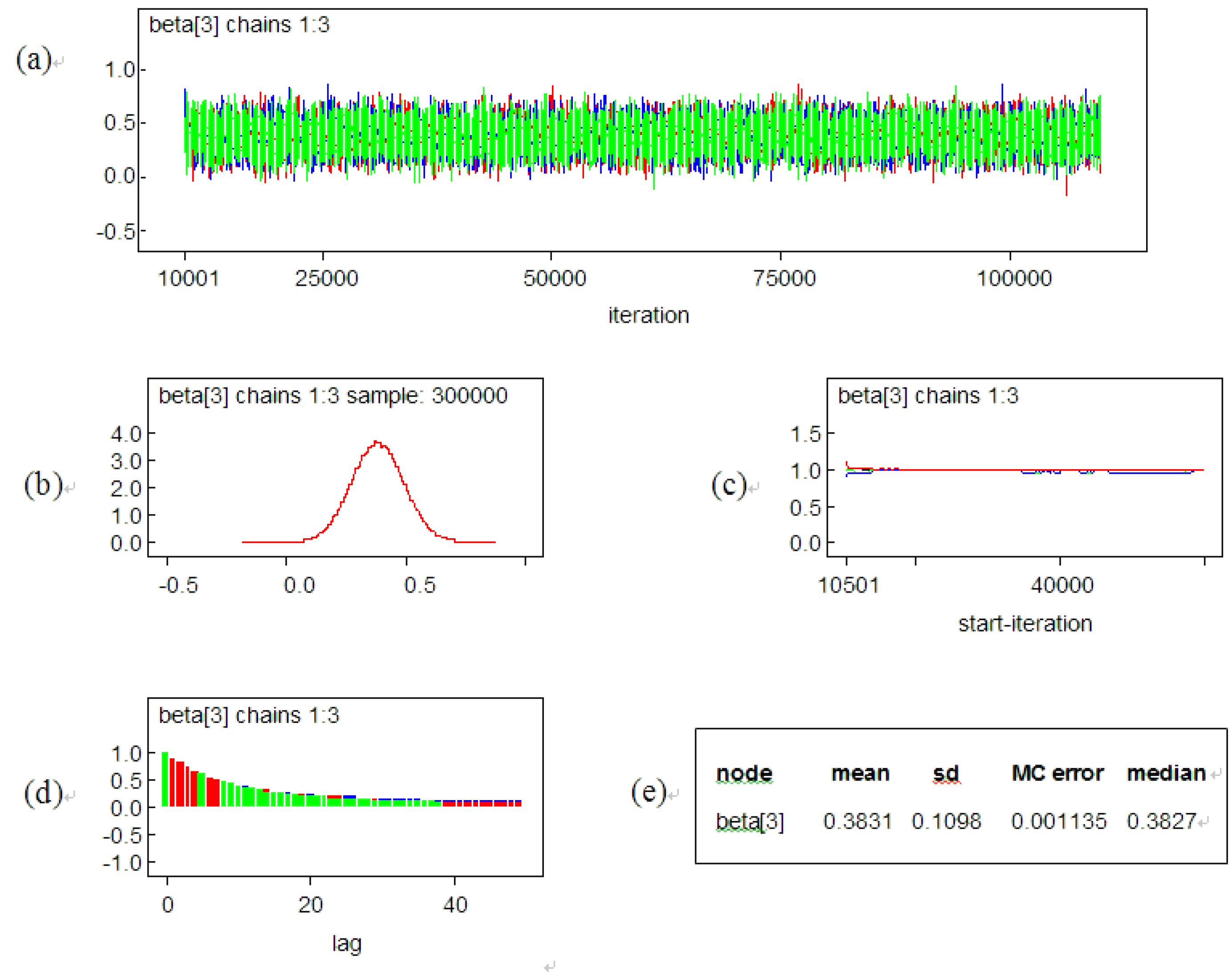
Bar density	−0.0184 (−0.1310, 0.0860)	0.3094 (0.1020, 0.5181)	0.3831 (0.1688, 0.6003)
Department store density	−0.0625 (−0.1593, 0.0234)	0.1928 (0.0027, 0.3797)	0.2119 (0.0338, 0.3878)
Policing	−0.1618 (−0.2489, −0.0794)	−0.0138 (−0.2151, 0.1853)	0.0264 (−0.1896, 0.2386)
$\psi$	NA	NA	0.5493 (0.2784, 0.8108)
DIC	4,982.890	742.030	736.462
$p_d$	5.963	102.164	101.470

presents the results of the three models fitted in WinBUGS. Model 1 is the non-spatial Poisson model without accounting for overdispersion and spatial structure (Equation (3)). Model 2 is the non-spatial Poisson model with only an unstructured random effects term $U\left(i\right)$ to account for overdispersion (Equation (5)). Model 3 is the spatial random effects model with an unstructured random effects term $U\left(i\right)$ and a structured random effects term $S\left(i\right)$ to account for overdispersion and spatial structure, respectively (Equation (4)). DICs for Model 2 and Model 3 are 742.030 and 736.462, as compared to 4982.890 for Model 1. Although Model 2 and Model 3 have about 105 additional effective parameters ($p_d$) for the random effects terms than Model 1, it is worth it in the sense that their DICs are far smaller. The much smaller DICs for Model 2 and Model 3 illustrate the necessity of accounting for overdispersion by random effects. In addition, Model 3 has a smaller DIC than Model 2 by 5.568, and can be considered more parsimonious than Model 2 because it has fewer $p_d$. Thus, Model 3 is better supported by our data than Model 2. The posterior mean of $\psi$ obtained from Model 3 is 0.5493. This demonstrates that about 55% of excess variability not explained by the covariates is due to spatially structured random variation. At the same time, unstructured random noise accounts for 45% of excess variability. Neither structured random variation nor unstructured random noise is dominating over other. This suggests that it is necessary to include both the structured and unstructured random effects in our model. In summary, a comparison of DICs for Model 1, Model 2 and Model 3 indicates that Model 3 best fit the data. Moreover, the posterior mean of $\psi$ further indicates that Model 3 is the best model among the three models as it considers both structured random variation and unstructured random noise, unlike the other two models.

In Model 1, three covariates are significant at the 95% credible interval (CI). They are population density, unemployment rate and policing. After accounting for overdispersion by the random effects term in Model 2 and Model 3, the unemployment rate and policing are no longer significant, while bar density and department store density become significant. This indicates that Model 1 incorrectly identifies the significance of some covariates. In addition, regression coefficients for bar density and department store density changed their signs in Model 2 and Model 3. Although Model 2 and Model 3 identify the same set of significant covariates, the precisions of regression coefficients for all the covariates other than department store density from Model 2 are overestimated compared to those from Model 3. These results provide further support for the claim that the spatial random effects model (Model 3) is superior to the non-spatial models (Model 1 and Model 2). Thus, if overdispersion and spatial autocorrelation exist but are not properly accounted for in the regression model, biased and even incorrect inferences can be derived. Our remaining analyses, therefore, are based solely on the spatial Poisson model (Model 3).

The results of the spatial Poisson model show that the unemployment rate and policing do not have a clear association with burglary risks. Population density is negatively correlated with burglary risks, while bar density and department store density are positively correlated with burglary risks. Neighborhoods show a 26.07% decrease in burglary risks with an increase of one standard deviation in population density (Equation (8)). At the same time, neighborhoods experience a 46.68% increase and a 23.60% increase in burglary risks with an increase of one standard deviation in bar density and department store density, respectively (Equations (9) and (10)). In all instances, all other covariates are held constant:

$$exp\left(-0.3020\right)-1=-0.2607$$

(8)

$$exp\left(0.3831\right)-1=0.4668$$

(9)

$$exp\left(0.2034\right)-1=0.2360$$

(10)

Figure 2 presents the distribution map of standardized burglary ratios (SBRs) at the neighborhood level. SBR is the crude ratio of the observed number of burglaries to the expected number. It is a measure of burglary risks. A neighborhood whose SBR is larger than 1.0 has more burglary incidents than expected. Three neighborhoods had a SBR of 0.0 as their observed burglary counts were all zero. About 33.3% (38 out of 114) of all the neighborhoods had a SBR higher than 1.0. Three of these neighborhoods had a SBR value larger than 9.0, indicating they had observed burglary counts more than nine times the expected.

Figure 3 illustrates the distribution map of burglary risks (posterior means of area-specific burglary risk $r\left(i\right)$) estimated by the spatial Poisson model (Model 3). Unlike SBR, the calculation of this measure of burglary risks takes account of the effects of covariates, structured random variation and unstructured random variation. This map clearly demonstrates the spatial smoothing effect from the Bayesian random effects modeling. Specifically, no neighborhood shows a risk of 0.0. This is more representative of true risks as burglary risk is unlikely to be zero in any of the neighborhoods. In addition, one of the neighborhoods in the bottom right corner of Figure 2 that in Figure 2 has a SBR larger than 1.0 now has a value lower than 1.0. This spatial smoothing helps to stabilize risk estimates. It is implemented through the spatial random effects term in the Bayesian spatial random effects model that enables neighborhoods to borrow information from their neighbors.

Figure 4 maps the posterior probabilities of neighborhoods having a burglary risk larger than 1.0. Unlike burglary risks mapped in Figure 3 that do not account for variance, posterior probabilities account for the variance of area-specific burglary risks. They measure the strength that the neighborhood-specific burglary risk is higher 1.0. For each neighborhood, this probability is equal to the proportion of simulations that assign it a risk greater than 1.0. Figure 4 indicates there are 31 neighborhoods having a posterior probability value higher than 0.80 (24 neighborhoods higher than 0.95). In disease mapping, Richardson et al. propose a decision rule to detect true raised-risk areas, i.e., using a value of around 0.7–0.8 as the threshold on the posterior probability [65]. Posterior means of burglary risks for these 31 neighborhoods are all larger than 1.0, as can been from Figure 3. These neighborhoods should be given adequate attention and further investigated by law enforcement departments and researchers.

5. Discussion

In our research, we used a Bayesian random effects modeling approach to explore the influence of neighborhood characteristics on burglary risks in Jianghan District, Wuhan, China. Overdispersion was present in the burglary data, as variance (5950.74) was more than 164 times the mean (36.10). Five covariates, i.e., population density, unemployment rate, bar density, department store density and policing, were assumed potential risk factors. Three models were used to fit the data. Model 1 (Equation (3)), without accounting for overdispersion, has a DIC of 4983. Model 2 (Equation (5)) and Model 3 (Equation (4)), which incorporate random effects to account for overdispersion, have a DIC of 742 and 736, respectively. Much of the differences in DICs result primarily from overdispersion. The larger reduction of DIC in Model 2 and Model 3 illustrates the necessity and importance of accounting for overdispersion when fitting models to small-area count data. Considering covariates, Model 1 identifies population density, the unemployment rate, and policing to be significant at the 95% credible interval. However, when overdispersion was accounted by the random effects in Model 2 and Model 3, the unemployment rate and policing were no longer significant, while bar density and department store density became significant. Model 1 incorrectly identified the significance of some covariates. This further confirms that overdispersion needs to be dealt with properly in small-area crime analysis. Model 2 and Model 3 identified the same set of significant covariates, but a relatively more accurate estimate of regression coefficients and a smaller DIC were obtained from Model 3 as shown in Table 2. This indicates that Model 3, accounting for spatial autocorrelation by including a spatially random effects term, is superior to Model 2, which does not account for spatial autocorrelation. In all, Model 3, incorporating both the unstructured and the structured random effects to account for overdispersion and spatial auto-correlation, is the best model. The posterior mean of $\psi$ (0.5493) shows that neither structured random variation nor unstructured random noise is dominating the other, further illustrating the necessity of incorporating both random effects terms. All these demonstrate that the spatial random effects model (Model 3) is superior to the non-spatial models (Model 1 and Model 2). Bayesian random effects modeling method provides a new way to understand the risk factors correlated with crime at a small-area scale, contributing to determining appropriate crime prevention and intervention strategies. Our study provides a contribution to the criminological literature as the Bayesian random effects modeling approach is still seldom used in crime analysis.

The results of this study suggest that burglary risks in Jianghan District, Wuhan, are significantly correlated with population density, bar density and department store density at the 95% credible interval. Population density has a negative association with burglary risks. It can lower burglary risks, possibly because large population density makes it easier to monitor residential buildings. Burglary risks are higher in neighborhoods that have a bar density above the average. This finding is consistent with prior studies showing that places with bars have more crime than places without bars [66]. Higher department store density is related to increased burglary risks in the Jianghan District. The unemployment rate is also positively correlated with burglary risks. This is in accordance with social disorganization theory claiming that low socioeconomic status is usually positively correlated with crime, although the unemployment rate in our analysis is not significant. The reason why it is not significant may be that unemployment rate acts as a proxy for socioeconomic status in our paper. However, socioeconomic status is complex and cannot be fully represented solely by the unemployment rate. Policing is also insignificant in our analysis. The reason may be that it can prevent crime but, on the other hand, it may also be a reaction to high-crime areas. Results also indicate that about 55% of excess variability in burglary risks is due to spatially structured random variation. The remaining 45% is resulting from unstructured random noise.

We mapped burglary risks estimated by the random effects model and demonstrated the spatial smoothing effect acquired by borrowing strength from neighboring areas, which stabilized risk estimates (Figure 3). Posterior probabilities of neighborhoods having a burglary risk greater than 1.0 were also mapped (Figure 4). Depending on specific situations or research questions, this value can be altered in our Bayesian random effects model. For example, posterior probabilities of neighborhoods having a burglary risk greater than 9.0 can also be estimated. Figure 4 and Figure 3 can be used together in practice to provide reference for crime prevention and control. In sum, the Bayesian random effects modeling approach is appropriate to model small-area discrete count data that may exhibit a small amount, overdispersion and spatial autocorrelation.

6. Conclusions

This paper adds to our understanding of the relationship between burglary risks and neighborhood characteristics. The results of our study have direct and practical implications on police resource allocation and the evaluation of crime prevention and control programs. Police focusing on burglary incidents in Jianghan District should target operations toward neighborhoods that have a high density of bars and department stores. Neighborhoods whose burglary risks are greater than 1.0 (shown in Figure 3) and where posterior probabilities of burglary risks greater than 1.0 (shown in Figure 4) are high should be prioritized robustly for intervention and given adequate attention for further investigation.

This study also has some limitations. First, the study region was treated as a closed system and we did not consider influences from outside areas. Second, the findings of this study are limited to Jianghan District and may not be applicable elsewhere. Third, the burglary data were obtained from the 110 reporting system. They may not accurately reflect all the burglary occurrences due to non-reporting or under-reporting of crimes and data entry errors [67,68]. As for the covariates, we have assumed their effects are homogeneous over the study region. In reality, however, spatial impacts are not necessarily homogeneous. In addition, the unemployment rate may not be powerful enough to represent socioeconomic status. Also, some potential variables related to social disorganization theory and routine activity theory, such as ethnic heterogeneity, family disruption, residential mobility and built environment, were not included in this study as they were not available. Future work could extend the current analysis to study the temporal dynamics of burglary risks through a spatio-temporal modeling approach.

References

- Weisburd, D.; Bruinsma, G.J.; Bernasco, W. Units of analysis in geographic criminology: Historical development, critical issues, and open questions. In Putting Crime in Its Place; Springer: Berlin, Germany, 2009; pp. 3–31. [Google Scholar]
- Weir, R.; Bangs, M.; Britain, G. The Use of Geographic Information Systems by Crime Analysts in England and Wales; Home Office: London, UK, 2007. [Google Scholar]
- Archer, D.; Gartner, R. Violence and Crime in Cross-national Perspective; Yale University Press: New Haven, CT, USA, 1987. [Google Scholar]
- Faggiani, D.; Bibel, D.; Brensilber, D. Regional problem solving using the national incident based reporting system. In Solving Crime and Disorder Problems; Police Executive Research Forum: Washington, DC, USA, 2001; pp. 155–174. [Google Scholar]
- Baller, R.D.; Anselin, L.; Messner, S.F.; Deane, G.; Hawkins, D.F. Structural covariates of us county homicide rates: Incorporating spatial effects. Criminology 2001, 39, 561–588. [Google Scholar] [CrossRef]
- Cork, D. Examining space–time interaction in city-level homicide data: Crack markets and the diffusion of guns among youth. J. Quant. Criminol. 1999, 15, 379–406. [Google Scholar] [CrossRef]
- Baumer, E.; Lauritsen, J.L.; Rosenfeld, R.; Wright, R. The influence of crack cocaine on robbery, burglary, and homicide rates: A cross-city, longitudinal analysis. J. Res. Crime Delinquency 1998, 35, 316–340. [Google Scholar] [CrossRef]
- Taylor, R.B. Social order and disorder of street blocks and neighborhoods: Ecology, microecology, and the systemic model of social disorganization. J. Res. Crime Delinquency 1997, 34, 113–155. [Google Scholar] [CrossRef]
- Martin, D. Spatial patterns in residential burglary assessing the effect of neighborhood social capital. J. Contemp. Criminal Justice 2002, 18, 132–146. [Google Scholar] [CrossRef]
- Groff, E.R.; Weisburd, D.; Yang, S.-M. Is it important to examine crime trends at a local “micro” level?: A longitudinal analysis of street to street variability in crime trajectories. J. Quant. Criminol. 2010, 26, 7–32. [Google Scholar] [CrossRef]
- Smith, W.R.; Frazee, S.G.; Davison, E.L. Futhering the integration of routine activity and social disorganization theories: Small units of analysis and the study of street robbery as a diffusion process. Criminology 2000, 38, 489–524. [Google Scholar] [CrossRef]
- Law, J.; Haining, R. A bayesian approach to modeling binary data: The case of high-intensity crime areas. Geogr. Anal. 2004, 36, 197–216. [Google Scholar] [CrossRef]
- Morenoff, J.D.; Sampson, R.J.; Raudenbush, S.W. Neighborhood inequality, collective efficacy, and the spatial dynamics of urban violence. Criminology 2001, 39, 517–558. [Google Scholar] [CrossRef]
- Andresen, M.A. A spatial analysis of crime in vancouver, british columbia: A synthesis of social disorganization and routine activity theory. Can. Geogr./Le Géographe canadien 2006, 50, 487–502. [Google Scholar] [CrossRef]
- Malczewski, J.; Poetz, A. Residential burglaries and neighborhood socioeconomic context in london, ontario: Global and local regression analysis. Prof. Geogr. 2005, 57, 516–529. [Google Scholar] [CrossRef]
- Stein, R.E.; Conley, J.F.; Davis, C. The differential impact of physical disorder and collective efficacy: A geographically weighted regression on violent crime. GeoJournal 2015, 81, 1–15. [Google Scholar] [CrossRef]
- Anselin, L. Spatial Econometrics: Methods and Models; Kulwer Academic: Dordrecht, The Netherlands, 1988. [Google Scholar]
- Carlin, B.P.; Louis, T.A. Bayes and Empirical Bayes Methods for Data Analysis, 2nd ed.; Chapman and Hall: London, UK, 2000. [Google Scholar]
- Spiegelhalter, D.J.; Thomas, A.; Best, N.G.; Gilks, W.R. Bugs: Bayesian Inference Using Gibbs Sampling, version 0.50; Cambridge University, MRC Biostatistics Unit: Cambridge, UK, 1995. [Google Scholar]
- Clayton, D.; Kaldor, J. Empirical bayes estimates of age-standardized relative risks for use in disease mapping. Biometrics 1987, 43, 671–681. [Google Scholar] [CrossRef] [PubMed]
- Bernardinelli, L.; Clayton, D.; Pascutto, C.; Montomoli, C.; Ghislandi, M.; Songini, M. Bayesian analysis of space-time variation in disease risk. Stat. Med. 1995, 14, 2433–2443. [Google Scholar] [CrossRef] [PubMed]
- Lawson, A.B. Bayesian Disease Mapping: Hierarchical Modeling in Spatial Epidemiology; CRC Press: Boca Raton, FL, USA, 2013. [Google Scholar]
- Kim, H.; Oleson, J.J. A bayesian dynamic spatio-temporal interaction model: An application to prostate cancer incidence. Geogr. Anal. 2008, 40, 77–96. [Google Scholar] [CrossRef]
- Haining, R.; Law, J. Combining police perceptions with police records of serious crime areas: A modelling approach. J. R. Stat. Soc. Ser. A (Stat. Soc.) 2007, 170, 1019–1034. [Google Scholar] [CrossRef]
- Freisthler, B.; Weiss, R.E. Using bayesian space-time models to understand the substance use environment and risk for being referred to child protective services. Subst. Use Misuse 2008, 43, 239–251. [Google Scholar] [CrossRef] [PubMed]
- Wheeler, D.C.; Waller, L.A. Comparing spatially varying coefficient models: A case study examining violent crime rates and their relationships to alcohol outlets and illegal drug arrests. J. Geogr. Syst. 2009, 11, 1–22. [Google Scholar] [CrossRef]
- Levine, N.; Block, R. Bayesian journey-to-crime estimation: An improvement in geographic profiling methodology. Prof. Geogr. 2011, 63, 213–229. [Google Scholar] [CrossRef]
- Yu, Q.; Scribner, R.; Carlin, B.; Theall, K.; Simonsen, N.; Ghosh-Dastidar, B.; Cohen, D.; Mason, K. Multilevel spatio-temporal dual changepoint models for relating alcohol outlet destruction and changes in neighbourhood rates of assaultive violence. Geosp. Health 2008, 2, 161–172. [Google Scholar] [CrossRef] [PubMed]
- Cunradi, C.B.; Mair, C.; Ponicki, W.; Remer, L. Alcohol outlets, neighborhood characteristics, and intimate partner violence: Ecological analysis of a california city. J. Urban Health 2011, 88, 191–200. [Google Scholar] [CrossRef] [PubMed]
- Law, J.; Chan, P.W. Bayesian spatial random effect modelling for analysing burglary risks controlling for offender, socioeconomic, and unknown risk factors. Appl. Spat. Anal. Policy 2012, 5, 73–96. [Google Scholar] [CrossRef]
- Law, J.; Quick, M. Exploring links between juvenile offenders and social disorganization at a large map scale: A bayesian spatial modeling approach. J. Geogr. Syst. 2013, 15, 89–113. [Google Scholar] [CrossRef]
- Gracia, E.; López-Quílez, A.; Marco, M.; Lladosa, S.; Lila, M. Exploring neighborhood influences on small-area variations in intimate partner violence risk: A bayesian random-effects modeling approach. Int. J. Environ. Res. Public Health 2014, 11, 866–882. [Google Scholar] [CrossRef] [PubMed]
- Law, J.; Quick, M.; Chan, P. Bayesian spatio-temporal modeling for analysing local patterns of crime over time at the small-area level. J. Quant. Criminol. 2014, 30, 57–78. [Google Scholar] [CrossRef]
- Law, J.; Quick, M.; Chan, P.W. Analyzing hotspots of crime using a bayesian spatiotemporal modeling approach: A case study of violent crime in the greater toronto area. Geogr. Anal. 2015, 47, 1–19. [Google Scholar] [CrossRef]
- Gracia, E.; López-Quílez, A.; Marco, M.; Lladosa, S.; Lila, M. The spatial epidemiology of intimate partner violence: Do neighborhoods matter? Am. J. Epidemiol. 2015, 182, 58–66. [Google Scholar] [CrossRef] [PubMed]
- Knorr-Held, L. Bayesian modelling of inseparable space-time variation in disease risk. Stat. Med. 1999, 19, 2555–2567. [Google Scholar] [CrossRef]
- Mollié, A.; Gilks, W.; Richardson, S.; Spiegelhalter, D. Bayesian mapping of disease. Markov Chain Monte Carlo Pract. 1996, 1, 359–379. [Google Scholar]
- Wakefield, J.; Best, N.; Waller, L. Bayesian approaches to disease mapping. Spat. Epidemiol. Methods Appl. 2000. [Google Scholar] [CrossRef]
- Wuhan Municipal Bureau of Statistics. Wuhan Statistical Yearbook 2014; China Statistics Press: Beijing, China, 2014.
- Shaw, C.R.; McKay, H.D. Juvenile Delinquency and Urban Areas; University of Chicago Press: Chicago, IL, USA, 1942. [Google Scholar]
- Cohen, L.E.; Felson, M. Social change and crime rate trends: A routine activity approach. Am. Sociol. Rev. 1979, 44, 588–608. [Google Scholar] [CrossRef]
- Bursik, R.J. Social disorganization and theories of crime and delinquency: Problems and prospects. Criminology 1988, 26, 519–552. [Google Scholar] [CrossRef]
- Ackerman, W.V. Socioeconomic correlates of increasing crime rates in smaller communities. Prof. Geogr. 1998, 50, 372–387. [Google Scholar] [CrossRef]
- Felson, M.; Cohen, L.E. Human ecology and crime: A routine activity approach. Hum. Ecol. 1980, 8, 389–406. [Google Scholar] [CrossRef]
- Sherman, L.W.; Gartin, P.R.; Buerger, M.E. Hot spots of predatory crime: Routine activities and the criminology of place. Criminology 1989, 27, 27–56. [Google Scholar] [CrossRef]
- Jacobs, J. The Death and Life of Great American Cities; Random House: New York, NY, USA, 1961. [Google Scholar]
- Beasley, R.W.; Antunes, G. The etiology of urban crime an ecological analysis. Criminology 1974, 11, 439–461. [Google Scholar] [CrossRef]
- Rotolo, T.; Tittle, C.R. Population size, change, and crime in US cities. J. Quant. Criminol. 2006, 22, 341–367. [Google Scholar] [CrossRef]
- Roncek, D.W. Dangerous places: Crime and residential environment. Soc. Forces 1981, 60, 74–96. [Google Scholar] [CrossRef]
- Stark, R. Deviant places: A theory of the ecology of crime. Criminology 1987, 25, 893–910. [Google Scholar] [CrossRef]
- Roncek, D.W.; Maier, P.A. Bars, blocks, and crimes revisited: Linking the theory of routine activities to the empiricism of “hot spots”. Criminology 1991, 29, 725–753. [Google Scholar] [CrossRef]
- Evans, J.D. Straightforward Statistics for the Behavioral Sciences; Brooks/Cole Publishing: Pacific Grove, CA, USA, 1996. [Google Scholar]
- Dormann, C.F.; Elith, J.; Bacher, S.; Buchmann, C.; Carl, G.; Carré, G.; Marquéz, J.R.G.; Gruber, B.; Lafourcade, B.; Leitão, P.J. Collinearity: A review of methods to deal with it and a simulation study evaluating their performance. Ecography 2013, 36, 27–46. [Google Scholar] [CrossRef]
- Montgomery, D.C.; Peck, E.A.; Vining, G.G. Introduction to Linear Regression Analysis; John Wiley & Sons: New York, NY, USA, 2015. [Google Scholar]
- Bizeti, H.S.; de Carvalho, C.G.P.; de Souza, J.R.P.; Destro, D. Path analysis under multicollinearity in soybean. Braz. Arch. Biol. Technol. 2004, 47, 669–676. [Google Scholar] [CrossRef]
- Thomas, A.; Best, N.; Lunn, D.; Arnold, R.; Spiegelhalter, D. Geobugs User Manual; Medical Research Council Biostatistics Unit: Cambridge, UK, 2004. [Google Scholar]
- Besag, J.; York, J.; Mollié, A. Bayesian image restoration, with two applications in spatial statistics. Ann. Inst. Stat. Math. 1991, 43, 1–20. [Google Scholar] [CrossRef]
- Besag, J.; Kooperberg, C. On conditional and intrinsic autoregressions. Biometrika 1995, 82, 733–746. [Google Scholar]
- Gelman, A. Prior distributions for variance parameters in hierarchical models. Bayesian Anal. 2006, 1, 515–534. [Google Scholar]
- Best, N.G.; Arnold, R.A.; Thomas, A.; Waller, L.A.; Conlon, E.M. Bayesian models for spatially correlated disease and exposure data. In Proceedings of the Sixth Valencia International Meeting on Bayesian Statistics, Alcossebre, Spain, 6–10 June 1999; pp. 131–156.
- Spiegelhalter, D.J.; Best, N.G.; Carlin, B.P.; Van der Linde, A. Bayesian Deviance, the Effective Number of Parameters, and the Comparison of Arbitrarily Complex Models. Available online: http://www.sph.umn.edu/faculty1/wp-content/uploads/2012/11/rr98-009.pdf (accessed on 10 January 2016).
- Spiegelhalter, D.J.; Best, N.G.; Carlin, B.P.; Van Der Linde, A. Bayesian measures of model complexity and fit. J. R. Stat. Soc. Ser. B (Stat. Methodol.) 2002, 64, 583–639. [Google Scholar] [CrossRef]
- Akaike, H. Information theory and an extension of the maximum likelihood principle. In Selected Papers of Hirotugu Akaike; Springer: Berlin, Germany, 1998; pp. 199–213. [Google Scholar]
- Gelman, A.; Rubin, D.B. Inference from iterative simulation using multiple sequences. Stat. Sci. 1992, 7, 457–472. [Google Scholar] [CrossRef]
- Richardson, S.; Thomson, A.; Best, N.; Elliott, P. Interpreting posterior relative risk estimates in disease-mapping studies. Environ. Health Perspect. 2004, 112, 1016–1025. [Google Scholar] [CrossRef] [PubMed]
- Roncek, D.W.; Bell, R. Bars, blocks, and crimes. J. Environ. Syst. 1981, 11, 35–47. [Google Scholar] [CrossRef]
- Groff, E.R.; La Vigne, N.G. Mapping an opportunity surface of residential burglary. J. Res. Crime Delinq. 2001, 38, 257–278. [Google Scholar] [CrossRef]
- Robinson, M.B.; Mullen, K.L. Crime on campus: A survey of space users. Crime Prev. Community Saf. 2001, 3, 33–46. [Google Scholar] [CrossRef]