
The Size Distribution, Scaling Properties and Spatial Organization of Urban Clusters: A Global and Regional Percolation Perspective

 , , and
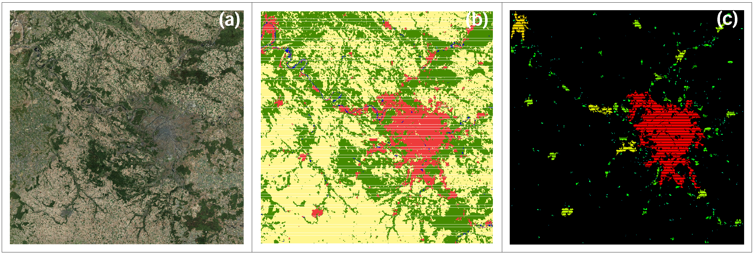
Abstract
:1. Introduction
2. City Clustering and Land Cover Data
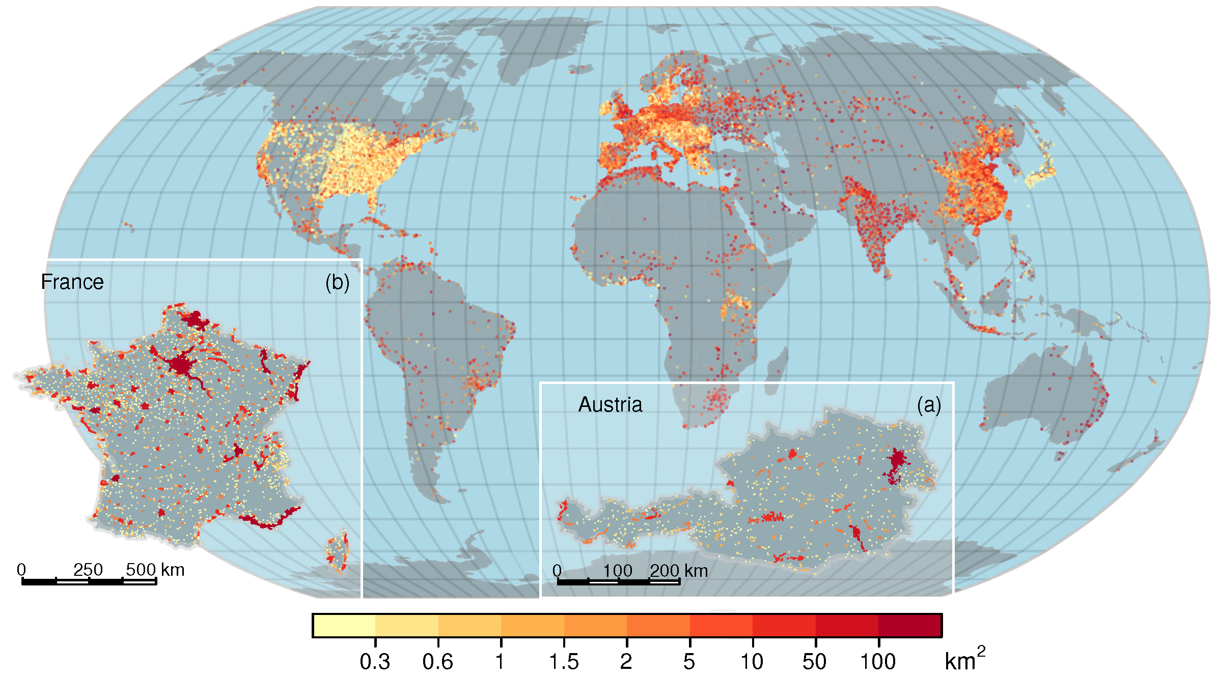
3. Global City Size Distribution
4. Percolation Transition and Size Distribution on the Country Scale
4.1. Percolation Transition
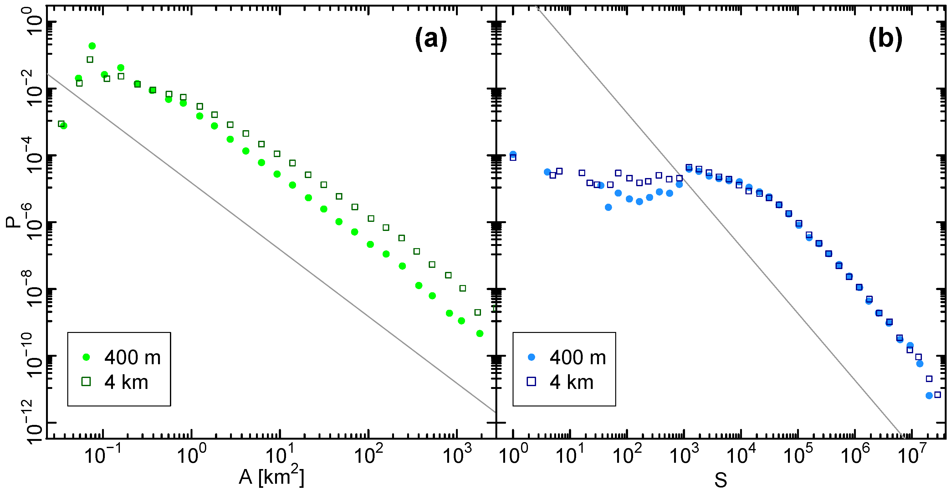
4.2. City Size Distribution
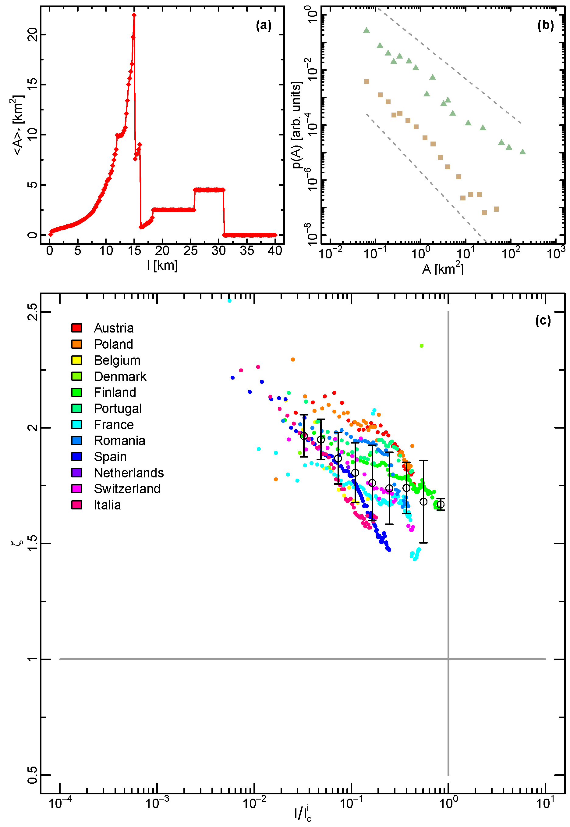
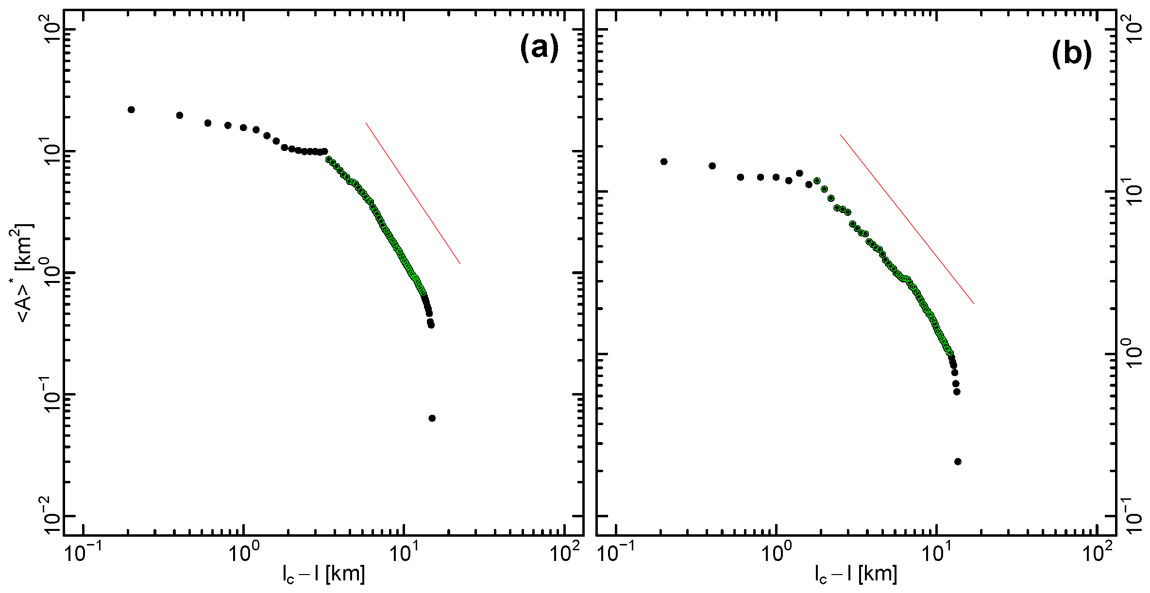
4.3. Average Size Scaling
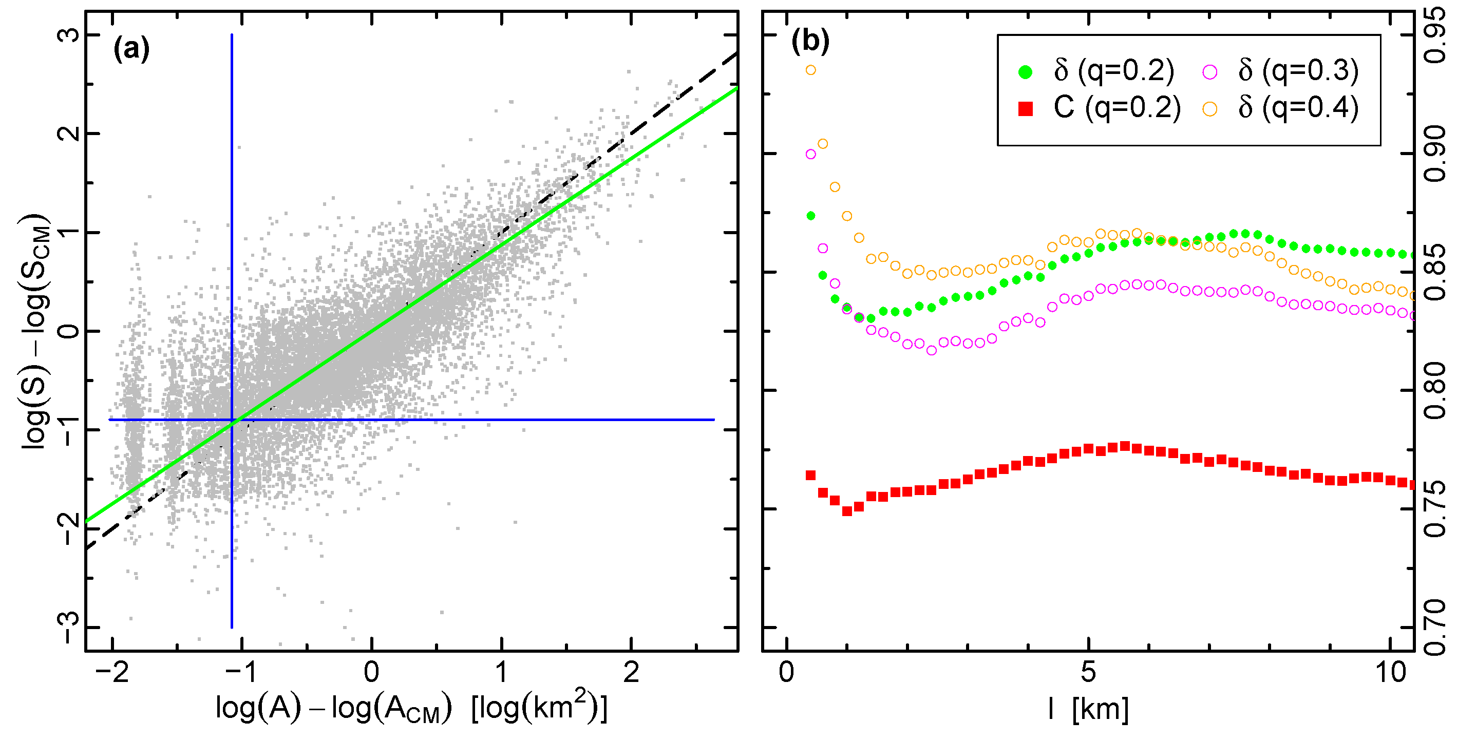
4.4. Taylor’s Law For City Size Distribution
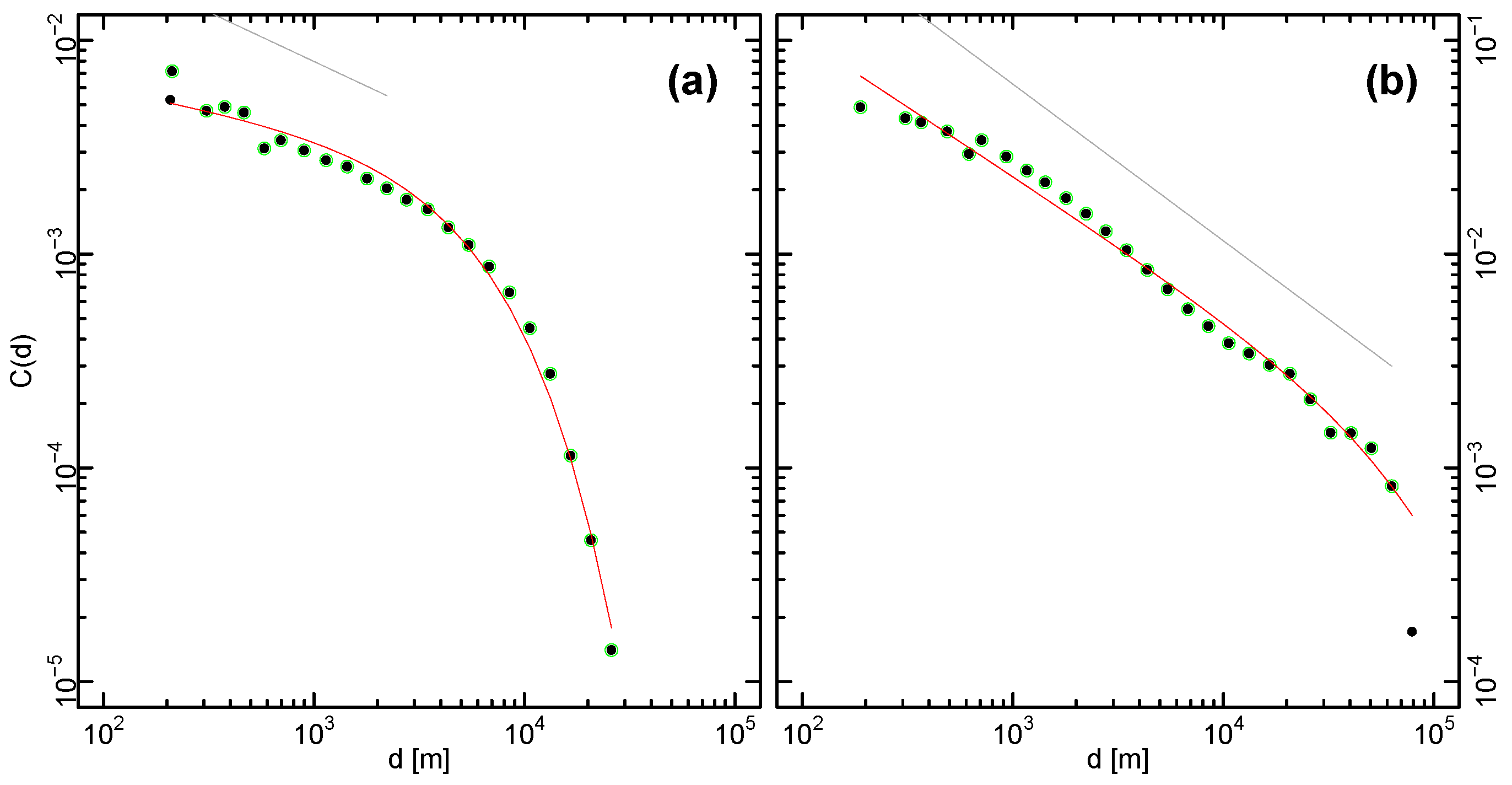
4.5. Spatial Correlations
5. Fundamental Urban Allometry—Relating Area and Population
6. Summary and Discussion
Acknowledgments
Author Contributions
Conflicts of Interest
References
- Auerbach, F. Das gesetz der bevölkerungskonzentration. Petermanns Geogr. Mitt. 1913, 59, 73–76. [Google Scholar]
- Rybski, D. Auerbach’s legacy. Environ. Plan. A 2013, 45, 1266–1268. [Google Scholar] [CrossRef]
- Zipf, G.K. Human Behavior and the Principle of Least Effort: An Introduction to Human Ecology (Reprint of 1949 Edition); Martino Publishing: Mansfield, CT, USA, 2012. [Google Scholar]
- Gibrat, R. Les Inégalités Économiques; Libraire du Recueil Sierey: Paris, France, 1931. [Google Scholar]
- Simon, H.A. On a class of skew distribution functions. Biometrika 1955, 42, 425–440. [Google Scholar] [CrossRef]
- Makse, H.A.; Andrade, J.S.; Batty, M.; Havlin, S.; Stanley, H.E. Modeling urban growth patterns with correlated percolation. Phys. Rev. E 1998, 58, 7054–7062. [Google Scholar] [CrossRef]
- Gabaix, X. Zipf’s law for cities: An explanation. Q. J. Econ. 1999, 114, 739–767. [Google Scholar] [CrossRef]
- Rybski, D.; Ros, A.G.C.; Kropp, J.P. Distance weighted city growth. Phys. Rev. E 2013, 87, 042114. [Google Scholar] [CrossRef] [PubMed]
- Eeckhout, J. Gibrat’s law for (All) cities. Am. Econ. Rev. 2004, 94, 1429–1451. [Google Scholar] [CrossRef]
- Kriewald, S.; Fluschnik, T.; Reusser, D.; Rybski, D. OSC: Orthodromic Spatial Clustering, R package version 1.0.0. Available online: https://CRAN.R-project.org/package=osc (accessed on 7 April 2011).
- Rozenfeld, H.D.; Rybski, D.; Andrade, J.S., Jr.; Batty, M.; Stanley, H.E.; Makse, H.A. Laws of population growth. Proc. Nat. Acad. Sci. USA 2008, 105, 18702–18707. [Google Scholar] [CrossRef] [PubMed]
- Stauffer, D.; Aharony, A. Introduction To Percolation Theory; Taylor & Francis: London, UK, 1994. [Google Scholar]
- ESA (European Space Agency). The Ionia GlobCover Project. GlobCover Land Cover 2009 v2.3. Available online: http://ionia1.esrin.esa.int (accessed on 21 August 2011).
- Center for International Earth Science Information Network (CIESIN), Columbia University; International Food Policy Research Institute (IFPRI), The World Bank; Centro Internacional de Agricultura Tropical (CIAT). Global Rural-Urban Mapping Project, Version 1 (GRUMPv1): Settlement Points. Website. 2011. Available online: http://sedac.ciesin.columbia.edu/data/dataset/grump-v1-settlement-points (accessed on 26 November 2011).
- Rozenfeld, H.D.; Rybski, D.; Gabaix, X.; Makse, H.A. The area and population of cities: New insights from a different perspective on cities. Am. Econ. Rev. 2011, 101, 2205–2225. [Google Scholar] [CrossRef]
- Zanette, D.H.; Manrubia, S.C. Role of intermittency in urban development: A model of large-scale city formation. Phys. Rev. Lett. 1997, 79, 523–526. [Google Scholar] [CrossRef]
- Batty, M. The size, scale, and shape of cities. Science 2008, 319, 769–771. [Google Scholar] [CrossRef] [PubMed]
- Schweitzer, F.; Steinbrink, J. Estimation of megacity growth—Simple rules versus complex phenomena. Appl. Geogr. 1998, 18, 69–81. [Google Scholar] [CrossRef]
- Kinoshita, T.; Kato, E.; Iwao, K.; Yamagata, Y. Investigating the rank-size relationship of urban areas using land cover maps. Geophys. Res. Lett. 2008, 35, L17405. [Google Scholar] [CrossRef]
- Arcaute, E.; Hatna, E.; Ferguson, P.; Youn, H.; Johansson, A.; Batty, M. Constructing cities, deconstructing scaling laws. J. R. Soc. Interface 2014, 12, 20140745. [Google Scholar] [CrossRef] [PubMed]
- Small, C.; Elvidge, C.D.; Balk, D.; Montgomery, M. Spatial scaling of stable night lights. Remote Sens. Environ. 2011, 115, 269–280. [Google Scholar] [CrossRef]
- Bunde, A.; Havlin, S. (Eds.) Fractals and Disordered Systems; Springer-Verlag: New York, NY, USA, 1991.
- Berry, B.J.L.; Okulicz-Kozaryn, A. The city size distribution debate: Resolution for US urban regions and megalopolitan areas. Cities 2012, 29, S17–S23. [Google Scholar] [CrossRef]
- Makse, H.A.; Havlin, S.; Stanley, H.E. Modeling urban-growth patterns. Nature 1995, 377, 608–612. [Google Scholar] [CrossRef]
- Bitner, A.; Holyst, R.; Fialkowski, M. From complex structures to complex processes: Percolation theory applied to the formation of a city. Phys. Rev. E 2009, 80, 037102. [Google Scholar] [CrossRef] [PubMed]
- Murcio, R.; Sosa-Herrera, A.; Rodriguez-Romo, S. Second-order metropolitan urban phase transitions. Chaos Soliton Fract. 2013, 48, 22–31. [Google Scholar] [CrossRef]
- Arcaute, E.; Molinero, C.; Hatna, E.; Murcio, R.; Vargas-Ruiz, C.; Masucci, P.; Batty, M. Regions and Cities in Britain through Hierarchical Percolation. Available online: http://arxiv.org/abs/1504.08318v2 (accessed on 10 July 2016).
- Clauset, A.; Shalizi, C.R.; Newman, M.E.J. Power-Law distributions in empirical data. SIAM Rev. 2009, 51, 661–703. [Google Scholar] [CrossRef]
- Vuong, Q.H. Likelihood ratio tests for model selection and non-nested hypotheses. Econometrica 1989, 57, 307–333. [Google Scholar] [CrossRef]
- Stanley, H.E. Scaling, universality, and renormalization: Three pillars of modern critical phenomena. Rev. Mod. Phys. 1999, 71, S358–S366. [Google Scholar] [CrossRef]
- Taylor, L.R. Aggregation, variance and mean. Nature 1961, 189, 732–735. [Google Scholar] [CrossRef]
- Smith, H.F. An empirical law describing heterogeneity in the yields of agricultural crops, Part: 1. J. Agric. Sci. 1938, 28, 1–23. [Google Scholar] [CrossRef]
- de Menezes, M.A.; Barabasi, A.L. Fluctuations in network dynamics. Phys. Rev. Lett. 2004, 92, 028701. [Google Scholar] [CrossRef] [PubMed]
- Eisler, Z.; Bartos, I.; Kertész, J. Fluctuation scaling in complex systems: Taylor’s law and beyond. Adv. Phys. 2008, 57, 89–142. [Google Scholar] [CrossRef]
- Bates, D.M.; DebRoy, S. R-Documentation: Nonlinear Least Squares. Available online: http://stat.ethz.ch/R-manual/R-patched/library/stats/html/nls.html (accessed on 7 April 2011).
- Weinrib, A. Long-range correlated percolation. Phys. Rev. B 1984, 29, 387–395. [Google Scholar] [CrossRef]
- Prakash, S.; Havlin, S.; Schwartz, M.; Stanley, H.E. Structural and dynamic properties of long-range correlated percolation. Phys. Rev. A 1992, 46, R1724–R1727. [Google Scholar] [CrossRef] [PubMed]
- Bettencourt, L.; West, G. A unified theory of urban living. Nature 2010, 467, 912–913. [Google Scholar] [CrossRef] [PubMed]
- Batty, M. Defining city size. Environ. Plan. B-Plan. Des. 2011, 38, 753–756. [Google Scholar] [CrossRef]
- Rybski, D.; Reusser, D.E.; Winz, A.L.; Fichtner, C.; Sterzel, T.; Kropp, J.P. Cities as nuclei of sustainability? Environ. Plan. B 2016. [Google Scholar] [CrossRef]
- Sutton, P.; Roberts, D.; Elvidge, C.; Baugh, K. Census from Heaven: An estimate of the global human population using night-time satellite imagery. Int. J. Remote Sens. 2001, 22, 3061–3076. [Google Scholar] [CrossRef]
- Potere, D.; Schneider, A.; Angel, S.; Civco, D.L. Mapping urban areas on a global scale: which of the eight maps now available is more accurate? Int. J. Remote Sens. 2009, 30, 6531–6558. [Google Scholar] [CrossRef]
- Zhou, B.; Rybski, D.; Kropp, J.P. On the statistics of urban heat island intensity. Geophys. Res. Lett. 2013, 40, 5486–5491. [Google Scholar] [CrossRef]
- Jefferson, M. The law of the primate city. Geogr. Rev. 1939, 29, 226–232. [Google Scholar] [CrossRef]
- Arcaute, E.; Hatna, E.; Ferguson, P.; Youn, H.; Johansson, A.; Batty, M. Constructing cities, deconstructing scaling laws. J. R. Soc. Interface 2014, 12, 20140745. [Google Scholar] [CrossRef] [PubMed]
- Pisarenko, V.F.; Sornette, D. Robust statistical tests of Dragon-Kings beyond power law distributions. Eur. Phys. J. Spec. Top. 2012, 205, 95–115. [Google Scholar] [CrossRef]
- Pumain, D.; Moriconi-Ebrard, F. City size distributions and metropolisation. GeoJournal 1997, 43, 307–314. [Google Scholar] [CrossRef]


© 2016 by the authors; licensee MDPI, Basel, Switzerland. This article is an open access article distributed under the terms and conditions of the Creative Commons Attribution (CC-BY) license (http://creativecommons.org/licenses/by/4.0/).
Share and Cite
Fluschnik, T.; Kriewald, S.; García Cantú Ros, A.; Zhou, B.; Reusser, D.E.; Kropp, J.P.; Rybski, D. The Size Distribution, Scaling Properties and Spatial Organization of Urban Clusters: A Global and Regional Percolation Perspective. ISPRS Int. J. Geo-Inf. 2016, 5, 110. https://0-doi-org.brum.beds.ac.uk/10.3390/ijgi5070110
Fluschnik T, Kriewald S, García Cantú Ros A, Zhou B, Reusser DE, Kropp JP, Rybski D. The Size Distribution, Scaling Properties and Spatial Organization of Urban Clusters: A Global and Regional Percolation Perspective. ISPRS International Journal of Geo-Information. 2016; 5(7):110. https://0-doi-org.brum.beds.ac.uk/10.3390/ijgi5070110
Chicago/Turabian StyleFluschnik, Till, Steffen Kriewald, Anselmo García Cantú Ros, Bin Zhou, Dominik E. Reusser, Jürgen P. Kropp, and Diego Rybski. 2016. "The Size Distribution, Scaling Properties and Spatial Organization of Urban Clusters: A Global and Regional Percolation Perspective" ISPRS International Journal of Geo-Information 5, no. 7: 110. https://0-doi-org.brum.beds.ac.uk/10.3390/ijgi5070110