Integrating Logistic Regression and Geostatistics for User-Oriented and Uncertainty-Informed Accuracy Characterization in Remotely-Sensed Land Cover Change Information

Abstract

Accuracy is increasingly recognized as an important dimension in geospatial information and analyses. A strategy well suited for map users who usually have limited information about map lineages is proposed for location-specific characterization of accuracy in land cover change maps. Logistic regression is used to predict the probabilities of correct change categorization based on local patterns of map classes in the focal three by three pixel neighborhood centered at individual pixels being analyzed, while kriging is performed to make corrections to regression predictions based on regression residuals at sample locations. To promote uncertainty-informed accuracy characterization and to facilitate adaptive sampling of validation data, standard errors in both regression predictions and kriging interpolation are quantified to derive error margins in the aforementioned accuracy predictions. It was found that the integration of logistic regression and kriging leads to more accurate predictions of local accuracies through proper handling of spatially-correlated binary data representing pixel-specific (in)correct classifications than kriging or logistic regression alone. Secondly, it was confirmed that pixel-specific class labels, focal dominances and focal class occurrences are significant covariates for regression predictions at individual pixels. Lastly, error measures computed of accuracy predictions can be used for adaptively and progressively locating samples to enhance sampling efficiency and to improve predictions. The proposed methods may be applied for characterizing the local accuracy of categorical maps concerned in spatial applications, either input or output.

1. Introduction

The provision of spatio-temporal land cover information is becoming increasingly important for landscape ecology and environmental monitoring. For example, it is necessary to have accurate information about land cover dynamics in order to quantify the extent and rate of land cover change and develop models to relate change-driving processes to observed landscape changes. Relevant case studies from the northern Mediterranean Basin, the European Alps and Inner Mongolia can be found in Millington et al. [1], Rutherford et al. [2] and Wu et al. [3], respectively.

Spatio-temporal land cover information may be acquired and derived from the combined use of field survey data and remotely-sensed images through statistical and other pattern analysis techniques in a semi-automatic fashion. Fuller et al. [4] examined issues concerning the detection, measurement and characterization of landscape changes by remote sensing and other means, while Chen et al. [5] described an effective and feasible strategy for operational global land cover mapping at 30-m resolution. Land cover information can be represented as categorical maps (or area-class maps) [6], either by polygons in vector format or contiguous blocks of grid cells in raster format.

While land cover is often static or persistent, information about land cover dynamics is also frequently consumed. Change detection results include binary maps of change and no-change types and categorical maps depicting specific “from-to” change classes; here, we refer to the latter case as change categorization, which can be considered a synonym to change detection, without causing confusion. Clearly, classification here refers to categorization of both static and changing cover types and is thus used interchangeably with change categorization in this paper, unless stated otherwise.

Land cover information is, however, imperfect, because it is not directly measurable, but results from interpretative and predictive processes that are subject to inherent subjectivity, inaccuracy and complexity. Lechner et al. [7] demonstrated the urgency to address spatial uncertainty in classification maps as standard practice in landscape ecology. Congalton et al. [8] highlighted the need for clear and uniform definitions of the classification scheme in global land cover mapping. It is thus crucial to characterize and analyze accuracy in land cover information so that derivatives, and analysis results based on such imperfect information can be scrutinized in terms of scientific replicability and practical usability. Olofsson et al. [9] provided practitioners with a set of “good practice” recommendations for designing and implementing accuracy assessment for change maps and estimating areas of different classes based on the reference sample data.

Issues of accuracy concern metrics, description, propagation and management of accuracy in land cover information. In this paper, we focus on the accuracy description. Accuracy in categorical maps can be described using epsilon error bands for the boundary position and confusion matrices for labeling, respectively. Although epsilon bands are useful for describing boundary inaccuracy, they are viewed as by-products of uncertainty in classification; thus, they will not be treated in this paper. The focus here is classification accuracy. Statistical measures of accuracy in land cover and other categorical information are mostly probabilistic (i.e., percent correctly-classified (PCC) pixels and per-class user’s accuracy). Such statistical measures of accuracy imply crisp sets in class definition and labeling, although fuzzy sets [10] may be used for measuring and representing uncertainty, in particular that concerning inherently vague classes, such as ecotones.

Accuracy measures derived from error matrices are usually global (e.g., PCCs and kappa coefficients of agreement) or class-stratified ones (e.g., user’s accuracy for individual classes) [9,11], without acknowledging spatial variation in classification accuracy, which is known to be spatially varied, as shown by Foody [12]. This paper seeks to quantify local classification accuracy in the context of change categorization. Location-specific predictions of classification accuracy provide information about the spatial variation of accuracy and can support exploratory and diagnostic analysis of factors influencing classification accuracy.

In general, there are two broad types of approaches to local accuracy quantification in land cover change information, depending on the availability and variety of source data and metadata, which can be used to assist accuracy characterization in addition to the maps being tested. One is producers’ approaches by which accuracy measures are derived from various source data involved in the production of land cover information, including multi-date images, training and testing samples, ancillary data and the derived maps of classification and change categorization. The other is users’ approaches in which data available for accuracy assessment are barely more than certain validation samples (for accuracy assessment) and the maps to be assessed. For the former, there are methods of probabilistic intervals (derived from single-date probabilistic classification accuracies) [13], maximum posteriori probabilities (used as surrogates of classification accuracy measures) [14,15] and re-sampling (which can map misclassification probabilities based on training samples and kriging) [16]. This paper extends the strategy of the latter, as follows.

For the users’ approaches, there are methods based on interpolation and regression analysis. Firstly, interpolation may be performed to predict probabilities of correct classification at unsampled locations, given a set of validation data. For this, indicator kriging, a kind of geostatistical interpolation method, can be used on the basis of validation samples and their indicator transforms to generate probability surfaces. For example, kriging was employed for mapping misclassification probability by Steele et al. [16]. Clearly, kriging will be a valuable tool for mapping local classification accuracy as spatial dependence is incorporated, with measures of uncertainty in predictions derived as kriging variance. Such uncertainty information will be useful, as we will discuss later. Secondly, logistic regression based on landscape pattern indices and other explanatory variables (covariates) has been proposed for estimating the probabilities of (in)correct classification, as described by researchers, including Smith et al. [17], Smith et al. [18] and Oort et al. [19]. It was found that certain landscape characteristics, such as high land cover heterogeneity and small patch size, result in pixels being harder to classify (thus lower accuracy) [17,18,19]. Clearly, both kriging and logistic regression may be explored for location-specific quantification of accuracy in change categorization.

This paper seeks to integrate the users’ approaches mentioned previously by combing regression and kriging for accuracy prediction in the context of change detection. This is done by predicting local probabilistic accuracy measures based on logistic regression followed by kriging for deriving corrections to regressed probabilities based on regression residuals evaluated at validation samples. In combined logistic-regression-kriging, logistic regression works by exploring and utilizing information conveyed by covariation between observed classification (in)correctness and local patterns of class occurrences in the map being evaluated, while kriging seeks to extract additional information contained in spatially-correlated regression residuals. The combined logistic-regression-kriging can be implemented either with fuller treatment of spatial correlation in both regression and kriging or just partially through kriging of regression residuals, as will be tested in this paper.

There is some research on using logistic regression to derive probabilistic estimates of accuracy in a change detection context by exploring relationships between the occurrences of erroneous change detection and various covariates, including single-date classification accuracy estimates, spectral data, spatial locations and landscape characteristics, as reported in Burnicki [20]. There is rarely any research on using, directly, local patterns of land cover change in the map being assessed as covariates for accuracy prediction based on logistic regression in the context of limited metadata, let alone those research efforts that explore spatial correlation through combined logistic-regression-kriging for improved accuracy predictions. In kriging with the regression residual, we need to clarify how nonstationary regionalized variables, such as the occurrences of (in)correct classification, should be handled. These provide important impetus for the paper and represent its major novelty.

It is important to recognize that accuracy measures derived from regression and kriging are only approximate, subject to validation samples (their numbers, distributions and accuracy), regression validity (model selection and covariates’ accuracy) and the presence and handling of spatial correlation in spatial binary data. Thus, it is important to demarcate how consistently the estimated accuracy measures are derived from predictions. This can be done by quantifying uncertainty, as measured by variance or its square root, standard error (SE), in predicted local accuracies. We can then use such information to identify locations where extra samples may be optimally placed to reduce uncertainty in accuracy predictions, and to build up adaptive sampling strategies for collecting validation data progressively, given existing validation samples, budgets for extra sampling and required precision in predictions. In this paper, variance values in regression predictions and residual kriging are estimated and combined to indicate uncertainty concerning local accuracy predictions.

In summary, the major contributions of this paper include:

(1)

Promoting a user-oriented strategy for local accuracy characterization in land cover change information through combined logistic regression and kriging based on validation samples and local-scale patterns of class occurrences in the maps being assessed.

(2)

Exploring significant covariates used to predict local accuracy by logistic regression, while logistic-regression-kriging procedures (with or without treatment of spatial correlation in logistic regression) are compared for their flexible use in applications depending on the range and strength of the spatial correlation in observed (in)correct classifications.

(3)

Investigating the effectiveness of adaptive sampling based on standard errors computed of accuracy predictions to enhance sampling efficiency and to increase prediction accuracy.

In Section 2, we will first describe indicator geostatistics for predicting local accuracies. This is followed by a description of logistic regression, by which probabilities of correct change categorization are predicted. Combined logistic-regression-kriging is described, in which spatial correlation in binary data concerning (in)correct classification is accommodated for the estimation of regression coefficients and variogram parameters. Methods for SE estimation are also described along with different methods of accuracy predictions. Section 3 will describe an empirical study aiming to test alternative methods for accuracy predictions using sample data collected in the study area. Section 4 will conclude the paper with some summaries and outlooks.

2. Methods

2.1. Indicator Geostatistics

Spatial dependence is characteristic of many geospatial distributions, such as land cover types and transitions. Misclassification and erroneous change categorization derived from remotely-sensed images are also likely spatially correlated. In geostatistics, such spatially-correlated distributions are described and modeled as regionalized variables [21,22]. Further, we can call an ensemble of random variables {Z(x₁), …, Z(x_n)} (x∈A, A being the problem domain) a random field (RF), if n locations {x₁, …, x_n | x∈A} are used to discretize the problem domain A; at a particular location x, Z(x) is a random variable (RV). Without causing confusion, we may denote the RF {Z(x), x∈A} simply by Z. To better differentiate interval/ratio RFs from nominal/ordinal RFs, we often denote the latter (e.g., land cover and other nominal fields [6]) as C as opposed to Z for the former. A nominal field C takes values in a series of class labels say {1, 2, …, K}, if K denotes the number of classes deemed possible in the domain A. Usually, a scalar RF is denoted in upper case, say C, with lower case c for its realizations (values).

As the focus of this paper is on binary correctness/incorrectness in categorical data (i.e., land cover change types), we need to discuss indicator geostatistics [21]. Below, we describe indicator variables and variograms briefly. For a categorical variable C(x), the indicator variable I(x) can be defined, in general, over a domain A by:

$$I\left(x\right)=\{\begin{array}{l}1, \mathrm{if} \widehat{C}\left(x\right)=C\left(x\right)\\ 0, \mathrm{otherwise}\end{array}$$

(1)

where $C\left(x\right)$ and $\widehat{C}\left(x\right)$ represent true and predicted land cover change types, respectively, at location x ($x\in A$). Equation (1) states that I(x) is 1 if x is correctly classified, 0 otherwise. This is essentially a binary coding of (in)correct classifications of sampled locations.

According to the theory of regionalized variables, a geostatistical data model for I(x) at x is such that I(x) is a sum of deterministic mean $\mathsf{\pi }$ and stochastic residual$\mathsf{\epsilon }\left(x\right)$:

$$I\left(x\right)=\mathsf{\pi }+\mathsf{\epsilon }\left(x\right)$$

(2)

If validation sampling is done properly, we may assert that the PCC measure calculated from a confusion matrix is a good estimation of the stationary and deterministic component, $\mathsf{\pi }$, as $\mathsf{\pi }$ = E[I(x)] = prob{I(x)} = 1.

Assuming second-order stationarity (which we will revisit in Section 2.3) in RF I, spatial covariance function, cov_I(h), for locations separated by a lag h is defined as:

$${\text{cov}}_I\left(h\right)=E\left[\right(I\left(x_s\right)-\mathsf{\pi }\left)\right(I\left(x_{s^{\prime }}\right)-\mathsf{\pi }\left)\right]=E\left[\mathsf{\epsilon }\right(x_s\left)\mathsf{\epsilon }\right(x_{s^{\prime }}\left)\right]$$

(3)

for $x_{\mathrm{s}}-x_{s^{\prime }}=h$, where the RF I, its deterministic component $\mathsf{\pi }$ and stochastic residual $\mathsf{\epsilon }$ are defined as in Equation (2). A variogram model ${\mathsf{\gamma }}_I\left(h\right)$ is related to the covariance model ${\text{cov}}_I\left(h\right)$ via: ${\mathsf{\gamma }}_I\left(h\right)={\text{cov}}_I\left(0\right)-{\text{cov}}_I\left(h\right)={\text{cov}}_I\left(0\right)\left(1-{\mathsf{\rho }}_I\left(h\right)\right)$, where ${\text{cov}}_I\left(0\right)$ is the variance (sill) of RF I and ${\mathsf{\rho }}_I\left(h\right)$ is the correlogram for I. Note that the subscripts in the notations above may be omitted without loss of clarity as they refer to RF I implicitly, unless otherwise indicated.

With variogram or covariance models fitted from empirical data properly, geostatistical prediction (commonly known as kriging) of RF I at unsampled locations may be performed. In general, kriging provides the best linear estimate $\widehat{I}\left(x_0\right)$ for the unknown value of I at unsampled locations x₀, which is determined by ensuring unbiasedness and minimum dispersion of the estimator. Simple (indicator) kriging may be performed when a stationary mean $\mathsf{\pi }$ over A is known. Specifically, this can be written as:

$$\widehat{I}\left(x_0\right)=p\{\widehat{C}\left(x_0\right)=C\left(x_0\right)\}=\mathsf{\pi }+{\displaystyle \sum }_{s=1}^n\mathsf{\lambda }\left(x_s\right)\left(i\left(x_s\right)-\mathsf{\pi }\right)$$

(4)

where $\widehat{I}\left(x_0\right)$ and $i\left(x_s\right)$ present the predicted value at x₀ and the data value at x_s, respectively, and λ(x_s) represents the weight assigned to data location x_s. Kriging variance, as a measure of the uncertainty in the prediction of $p\{\widehat{C}\left(x_0\right)=C\left(x_0\right)\}$ conditional to the data available, is computed:

$$\text{var}[\widehat{I}\left(x_0\right)]=\text{var}\left(I\right)-{\displaystyle \sum }_{s=1}^n{\mathsf{\lambda }}_{\mathrm{s}}\text{cov}\left(x_0-x_s\right)$$

(5)

where $\text{var}\left(I\right)={\text{cov}}_I\left(0\right)$ represents the sill of RF I’s variogram.

However, it is often the case that classification accuracies are varied by location, so that $\mathsf{\pi }$ in Equation (2) is better redefined by local means $\mathsf{\pi }\left(x\right)$(x∈A), which are found to be related in part to landscape shape indices in the neighborhood centered at the locations being assessed [19,20]. Thus, we should prescribe local means properly for geostatistical analysis of RF I and its prediction at unsampled locations, with Equation (2) re-written as:

$$I\left(x\right)=\mathsf{\pi }\left(x\right)+\mathsf{\epsilon }\left(x\right)$$

(6)

where $\mathsf{\pi }\left(x\right)$ and $\mathsf{\epsilon }\left(x\right)$ stand for the local mean and residual of I at x, respectively.

There are methods of incorporating some relevant covariates for the estimation of local means $\mathsf{\pi }\left(x\right)$, as prescribed in Equation (6). In linear geostatistics, the so-called universal kriging refers to the situations where local means are functions of spatial coordinates, while kriging with an external drift uses functions of an auxiliary RF as the locally-defined means, as discussed by Hengl et al. [22]. For indicator RF I, we cannot apply universal kriging directly, but may explore logistic regression to predict $\mathsf{\pi }\left(x\right)$ in Equation (6) based on relevant covariates, as shown in the next subsection.

2.2. Logistic Regression

As a kind of generalized linear modeling approach, logistic regression is a quantitative technique that can relate dependent binary variables (e.g., (in)correct classifications) with certain co-registered covariates. Past research has shown that class labels, heterogeneity, patch size and landscape dominance are significant covariates for predicting local accuracies, as described in Smith et al. [17], Smith et al. [18] and Oort et al. [19]. Here, we adapt some of the well-researched landscape shape indices and quantify them at a local scale (center pixel labels plus the4 focal 3 by 3 pixel neighborhood) to make them commensurate with the paper’s research objective of local accuracy quantification. The underlying rationales are that covariates quantified at the focal scale are more conformal to the dependent variable being analyzed, because the indicators registering (in)correct classification at individual pixels can be informed better within a focal neighborhood than further away and because accuracy-pattern relationships may not be linearly transferable across scales.

We propose using change class occurrence frequencies in the focal neighborhood as candidate covariates for regression analysis, while such pattern indices as heterogeneity and dominance can be derived from them. The class occurrences at pixel x are represented by the class probability vector p(x) in the focal neighborhood: p(x) = (p₁(x), p₂(x),…, p_K-1(x))^T, where the subscripts 1, 2, .., K-1 represents the class labels, p_k(x) the proportion of pixels in the 3 by 3 focal neighborhood belonging to class k, with superscript ^T indicating transpose and assuming that there are a total of K candidate classes under consideration. We need only to specify K − 1 of them, as there is a redundancy: p_K(x) = 1 − ${\sum }_{k=1}^{K-1}{p}_k\left(x\right)$.

Several focal-scale metrics of class occurrence patterns can be derived from the probability vector p defined above. Focal heterogeneity (HET) measures the heterogeneity of the focal neighborhood around each cell and equals the number of classes present in the focal neighborhood centered at the pixel being analyzed. A heterogeneity value of 1 indicates that the central pixel is located within a homogeneous block of pixels, while any value greater than 1 indicates that the pixel was located on a patch edge or in the class boundaries. Block size is defined as the number of contiguous pixels of the same class as the central pixel being analyzed, measuring the extent to which the local block is fragmented and reflecting class purity in a focal neighborhood, denoted L10B. Thirdly, we confine landscape dominance (DMG), which refers to landscape scale in Oort et al. [19], to a focal neighborhood, defining it as the difference between the logarithm of heterogeneity and the entropy of class occurrences in the focal neighborhood:

$$DMG\left(x\right)=\text{log}HET+{\displaystyle \sum }_{k=1}^K{p}_k\left(x\right)\text{log}{p}_k\left(x\right)$$

(7)

where p_k is the marginal probabilities of individual classes k in the focal neighborhood.

The candidate covariates mentioned previously are denoted as a vector F of length 1 + Q > 1: F(x) = (F₀(x) = 1, F₁(x), …, F_Q(x))^T, where Q is the total number of covariates used, except for the constant 1. For instance, we may have F₁ = HET and F₂ = DMG, etc. The locator x may or may not be specified along with F’s without loss of clarity in the text below.

For the indicator RF {I(x), x∈A} described in the previous subsection, its local means are related through logit models to the vectors F, a set of covariates (e.g., pattern indices of local class occurrences). In other words, the probability of correct classification at a location (say pixel x), $\mathsf{\pi }\left(x\right)=prob\left\{I\left(x\right)=1\right\}$, depends on F(x) through a corresponding set of coefficients, $\mathsf{\beta }={\left({\mathsf{\beta }}_0,{\mathsf{\beta }}_1,\cdots ,{\mathsf{\beta }}_{\mathrm{Q}}\right)}^{\mathrm{T}}$. The log odds, called the logit (denoted η) of $\mathsf{\pi }\left(x\right)$, are linearly related to covariates F(x) = (1, F₁(x), …, F_Q(x))^T at location x:

$$\mathsf{\eta }\left(\mathsf{\pi }\left(x\right)\right)=\text{logit}\left(\mathsf{\pi }\left(x\right)\right)=\text{log}\frac{\mathsf{\pi }\left(x\right)}{1-\mathsf{\pi }\left(x\right)}=F{\left(x\right)}^{\mathrm{T}}\mathsf{\beta }$$

(8)

Estimates of the coefficients’ vector $\mathsf{\beta }$, $\widehat{\mathsf{\beta }}$, can be obtained by the Newton–Raphson method or through iterative re-weighted least squares with a linearized form of the logit link function for the sample data, as described in Agresti [23]. The system of equations is:

$$F^{\mathrm{T}}WF\mathsf{\beta }=F^{\mathrm{T}}W{\mathsf{\eta }}^{*}$$

(9)

where $W=D^T{V}^{-1}D$, ${\mathsf{\eta }}^{*}=\mathsf{\eta }+D^{-1}\left(i-\mathsf{\pi }\right)$, with vectors ${\mathsf{\eta }}^{*}$, $\mathsf{\eta }$, $i$ and $\mathsf{\pi }$ being the column vectors of ${\mathsf{\eta }}^{*}$, $\mathsf{\eta }$, $i$ and $\mathsf{\pi }$ at sample locations (suppose there are n sampled locations; these vectors are of length n each). Here, matrix $D=diag\left[{\mathsf{\pi }}_s\left(1-{\mathsf{\pi }}_s\right)\right]$, and assuming independence in the set of RVs (represented by I) at sampled locations, the variance and covariance matrix V is specified as:

$$V=\text{var}\left(I\right)=diag\left(v\left(x_s\right)\right)=diag\left[\mathsf{\pi }\left(x_s\right)\left(1-\mathsf{\pi }\left(x_s\right)\right)\right]$$

(10)

where subscript s represents locations x_s., s = 1, …, n, with n being the number of sampled locations in regression analysis. An iterative process of least squares provides the solution to $\mathsf{\beta }$. Further detail can be found in Agresti [23] and Gotway et al. [24]. In the limit of the iterative process, $\widehat{\mathsf{\beta }}$ converges to its maximum likelihood estimate, with its variance and covariance matrix derived as:

$$\text{cov}(\widehat{\mathsf{\beta }})={\left(F^{\mathrm{T}}WF\right)}^{-1}$$

(11)

as described in Agresti [23].

With $\widehat{\mathsf{\beta }}$ estimated, we can compute $\widehat{\mathsf{\eta }}\left(x_0\right)$ for an unsampled location x₀ using (8). Then, we can predict $\widehat{\mathsf{\pi }}\left(x_0\right)$ by the inverse of Equation (8):

$$\widehat{\mathsf{\pi }}(x_0)=\exp (F^{\mathrm{T}}\widehat{\mathsf{\beta }})/(1+\text{exp}(F^{\mathrm{T}}\widehat{\mathsf{\beta }}))$$

(12)

Obviously, different sets of covariates F give rise to different logit models, pointing to the issue of significance testing about covariates’ selection for regression analysis. For model selection, there is the deviance statistic:

$$D=-2\text{log}\wedge =-2{\displaystyle \sum }_{l=1}^{n_l}[i_l\text{ln}\left(\frac{{\widehat{\mathsf{\pi }}}_l}{i_l}\right)+\left(1-i_l\right)\text{ln}(\frac{1-{\widehat{\mathsf{\pi }}}_l}{1-i_l})]$$

(13)

where $i_l$ denotes the binomial variate for the l-th setting of the covariates, $l=1,\cdots ,n_l$(with $n_l$ being the maximum number of settings for vectors F’s), and ${\widehat{\mathsf{\pi }}}_l$ denotes the model estimate corresponding to $\text{probability }(i_l=1|F_l)$. Differences in the deviance values for the models were used to test the effect of incorporating additional covariates. The difference follows a chi-square distribution with degrees of freedom (df) equal to the difference in the numbers of covariates used in the base model and the alternative model, as described in Agresti [23]. Statistical significance is judged at a certain significance level, say 0.05.

As with the kriging variance shown in Equation (5), we can also compute variance (or standard error SE = $\sqrt{\text{variance}}$) in $\widehat{\mathsf{\pi }}\left(x\right)$ predicted from logistic regression. Variance in logistic regression predictions can be calculated as follows. For estimated values of the logit as by Equation (8), its variance is:

$$\text{var}\left(\widehat{\mathsf{\eta }}\left(x_0\right)\right)=\text{var}\left(\text{logit}\left(\widehat{\mathsf{\pi }}\left(x_0\right)\right)\right)=F^T\text{cov}(\widehat{\mathsf{\beta }})F$$

(14)

where $\text{cov}(\widehat{\mathsf{\beta }})$ is computed using Equation (11). Variance for the predicted probabilities $\widehat{\mathsf{\pi }}\left(x_0\right)$ can then be obtained by the delta method, as shown in Agresti [23]. Specifically, variance in $\mathsf{\pi }\left(x_0\right)$ is computed from the variance of $\mathsf{\eta }\left(x_0\right)$ using:

$$\text{var}\left[\mathsf{\pi }\left(x_0\right)\right]={\left({\mathsf{\pi }}^{\prime }\left(\mathsf{\eta }\left(x_0\right)\right)\right)}^2\text{var}\left(\mathsf{\eta }\left(x_0\right)\right)$$

(15)

where ${\mathsf{\pi }}^{\prime }\left(\mathsf{\eta }\right)$ is evaluated as (referring to Equation (12)):

$${\mathsf{\pi }}^{\prime }\left(\mathsf{\eta }\left(x_0\right)\right)=\frac{\partial \mathsf{\pi }}{\partial \mathsf{\eta }}=\mathsf{\pi }\left(x_0\right)\left(1-\mathsf{\pi }\left(x_0\right)\right)$$

(16)

Variance in $\widehat{\mathsf{\pi }}\left(x_0\right)$ can be computed by substituting $\widehat{\mathsf{\eta }}\left(x_0\right)$ and $\widehat{\mathsf{\pi }}\left(x_0\right)$ for $\mathsf{\eta }\left(x_0\right)$ and $\mathsf{\pi }\left(x_0\right)$, respectively.

2.3. Integrating Logistic Regression and Kriging while Accommodating Spatial Correlation

RF I’s variance and covariance matrix V (for a set of sampled locations) shown in Equation (10) is assumed to be diagonal, as binary data {$i\left(x_s\right)$, s = 1, ..., n} involved there are considered to be uncorrelated. However, (in)correctness in change categorization (represented by RF I) is often spatially correlated, and its proper handling is important for the estimation of both local accuracies and their stand errors in the context of logistic regression. The strategy promoted in this paper is a kind of regression-kriging tailored for binary data registering (in)correct change categorization: logistic regression for local probabilities of (in)correct classification is performed on certain covariates, with simple kriging applied for regression residuals. Specifically, after local means are determined through regression analysis, the residuals are transformed to standardized residuals to facilitate variogram modeling and kriging implementation; the kriged residual values and their variance estimates are back-transformed to the original data space. The corrected local predictions of RF I will be the sum of regressed local means and kriged residuals, while variance in corrected predictions will also be the sum of variances in predicted means and predicted residuals. In both logistic regression and kriging, spatial correlation is accommodated by proper variogram modeling via standardized residuals; for the regression part, V in Equation (10) can be specified iteratively with variogram modeling based on the standardized residuals. We describe the procedures below.

For logistic regression with spatial binary data, variogram modeling needs to be considered in combination with the specification of the nonstationary means. Indeed, when $\mathsf{\pi }\left(x\right)$ representing local means is spatially varied, as shown in Equation (6), the variance of $\mathsf{\epsilon }\left(x\right)$ will be non-constant, and as a consequence, we cannot model $\mathsf{\epsilon }\left(x\right)$ as a stationary RF [25]. In Section 2.1, stationarity in RF I was assumed, taking the whole problem domain as a whole and viewing the occurrences of (in)correct classification across the problem domain A as if they were realizations of an RV I(x) at any particular location x within A (because of the assumption of stationarity regarding RF I).

It is possible to compute standardized residuals:

$$e\left(x\right)=\left(I\left(x\right)-\mathsf{\pi }\left(x\right)\right)/\sqrt{\mathsf{\pi }\left(x\right)\left(1-\mathsf{\pi }\left(x\right)\right)}=\mathsf{\epsilon }\left(x\right)/\sqrt{\mathsf{\pi }\left(x\right)\left(1-\mathsf{\pi }\left(x\right)\right)}$$

(17)

where we can replace $\mathsf{\pi }\left(x\right)$ with $\widehat{\mathsf{\pi }}\left(x\right)$ to get $\widehat{e}\left(x\right)$ (i.e., the estimated version of $e\left(x\right)$). With standardized residuals, we can model their variograms say cov_e(h) and hence correlograms ${\mathsf{\rho }}_e\left(h\right)$, which can then be exploited to obtain variance and covariance matrix V of the RF I (as opposed to that in Equation (10)):

$$V=V_{\mathsf{\pi }}^{1/2}R{V}_{\mathsf{\pi }}^{1/2}$$

(18)

in which:

$$\begin{gathered} V_{\mathsf{\pi }}^{1/2}=diag[\sqrt{{\mathsf{\pi }}_1\left(1-{\mathsf{\pi }}_1\right)},\cdots ,\sqrt{{\mathsf{\pi }}_{\mathrm{n}}\left(1-{\mathsf{\pi }}_{\mathrm{n}}\right)}] \\ R=\left(R_{s,s^{\prime }}\right)=\left({\mathsf{\rho }}_e\left(x_s,x_{s^{\prime }}\right)\right) \end{gathered}$$

where n is the number of sampled locations as implied in Equation (10) and ${\mathsf{\rho }}_e\left(x_s,x_{s^{\prime }}\right)$ indicates the correlogram between data locations $x_s$ and $x_{s^{\prime }}$, which is obtained from standardized residuals, as shown in Equation (17).

With spatially-correlated binary data, regression coefficients $\mathsf{\beta }$ and correlation parameters $\mathsf{\alpha }$ (e.g., range, nugget and sill describing variograms) can be estimated using generalized estimating equation (GEE) approaches [26,27]. They are iterative procedures, alternating between updating estimates of $\mathsf{\beta }$ and those of $\mathsf{\alpha }$, until convergence. A challenge in adapting the GEE methodology to spatial data analysis is the selection of a sensible correlation structure, as some of the assumed correlation structures supported in existing GEE software systems are not designed for spatial data. In practice, we can iteratively update estimates of $\mathsf{\beta }$ based on iteratively-updated variogram model parameters, as in [24].

With the solution to regression coefficients $\mathsf{\beta }$ and correlation parameters $\mathsf{\alpha }$ (hence, R and V in Equation (18)) obtained as above, local accuracy measures can then be derived from applying the coefficient vector $\widehat{\mathsf{\beta }}$ to Equation (12). As in conventional logistic regression, we can apply the delta method (Equation (15)) to compute variance in predicted probabilities of correct classification at individual locations.

After derivation of local accuracy measures and associated variance by logistic regression, regression residuals can be densified over unsampled locations through kriging. Due to non-constant local means $\mathsf{\pi }\left(x\right)$ and variances $\mathsf{\pi }\left(x\right)\left(1-\mathsf{\pi }\left(x\right)\right)$, we cannot, however, do kriging with residuals {$\mathsf{\epsilon }\left(x\right)$} directly. Instead, we perform simple kriging using Equation (4) in the space of standardized residuals {e(x)}. We should use the fitted variogram model for e, ${\mathsf{\rho }}_e\left(h\right)$, to compute the elements of the variance and covariance matrix between the data locations x_s (s = 1, …, n): $R_{e\left(n,n\right)}=\left({\mathsf{\rho }}_e\left(x_s,x_{s^{\prime }}\right)\right)$. Elements of the vector of covariances between a location to be predicted (i.e., x₀) and the data locations x_s (s = 1, …, n) can be calculated similarly: $R_{e\left(0,n\right)}=\left(\mathsf{\rho }\left(x_0,x_1\right),\cdots ,\mathsf{\rho }\left(x_0,x_n\right)\right)$. Variance in $\widehat{e}\left(x_0\right)$ can be computed using Equation (5), but in the space of standardized residuals {e(x)} and with sill = cov(h = 0) = 1. The kriged residuals e(x₀) (by Equation (5)) are then back-transformed to $\mathsf{\epsilon }\left(x_0\right)$ via the inversion of Equation (17):

$$\widehat{\mathsf{\epsilon }}\left(x_0\right)=\sqrt{\widehat{\mathsf{\pi }}\left(x_0\right)\left(1-\widehat{\mathsf{\pi }}\left(x_0\right)\right)}\widehat{e}\left(x_0\right)$$

(19)

Variance in $\widehat{\mathsf{\epsilon }}\left(x_0\right)$ is computed as:

$$\text{var}\left(\widehat{\mathsf{\epsilon }}\left(x_0\right)\right)=\widehat{\mathsf{\pi }}\left(x_0\right)\left(1-\widehat{\mathsf{\pi }}\left(x_0\right)\right)\text{var}\left(\widehat{e}\left(x_0\right)\right)$$

(20)

Kriged residuals at unsampled locations are used as corrections to regression predictions of local accuracies. Specifically, prediction of I at an unsampled pixel x₀, $\widehat{p}\left(x_0\right)$, was done by adding the predicted residual $\widehat{\mathsf{\epsilon }}\left(x_0\right)$ (using Equation (19)) to the regression prediction $\widehat{\mathsf{\pi }}\left(x_0\right)$:

$$\widehat{p}\left(x_0\right)=\widehat{\mathsf{\pi }}\left(x_0\right)+\widehat{\mathsf{\epsilon }}\left(x_0\right)$$

(21)

where the local means are estimated using Equation (12), but with $\widehat{\mathsf{\beta }}$, which should be obtained from procedures that can handle spatial correlation via matrix V (Equation (18)). The value of SE in the corrected accuracy measures $\widehat{p}\left(x_0\right)$ is:

$$\text{SE}[\widehat{p}\left(x_0\right)]=\sqrt{\text{var}[\widehat{p}\left(x_0\right)]}=\sqrt{\text{var}[\widehat{\mathsf{\pi }}\left(x_0\right)]+\text{var}[\widehat{\mathsf{\epsilon }}\left(x_0\right)]}$$

(22)

where $\text{var}[\widehat{\mathsf{\pi }}\left(x_0\right)]$ and $\text{var}[\widehat{\mathsf{\epsilon }}\left(x_0\right)]$ are computed using Equations (15) and (20), respectively

3. Experiments

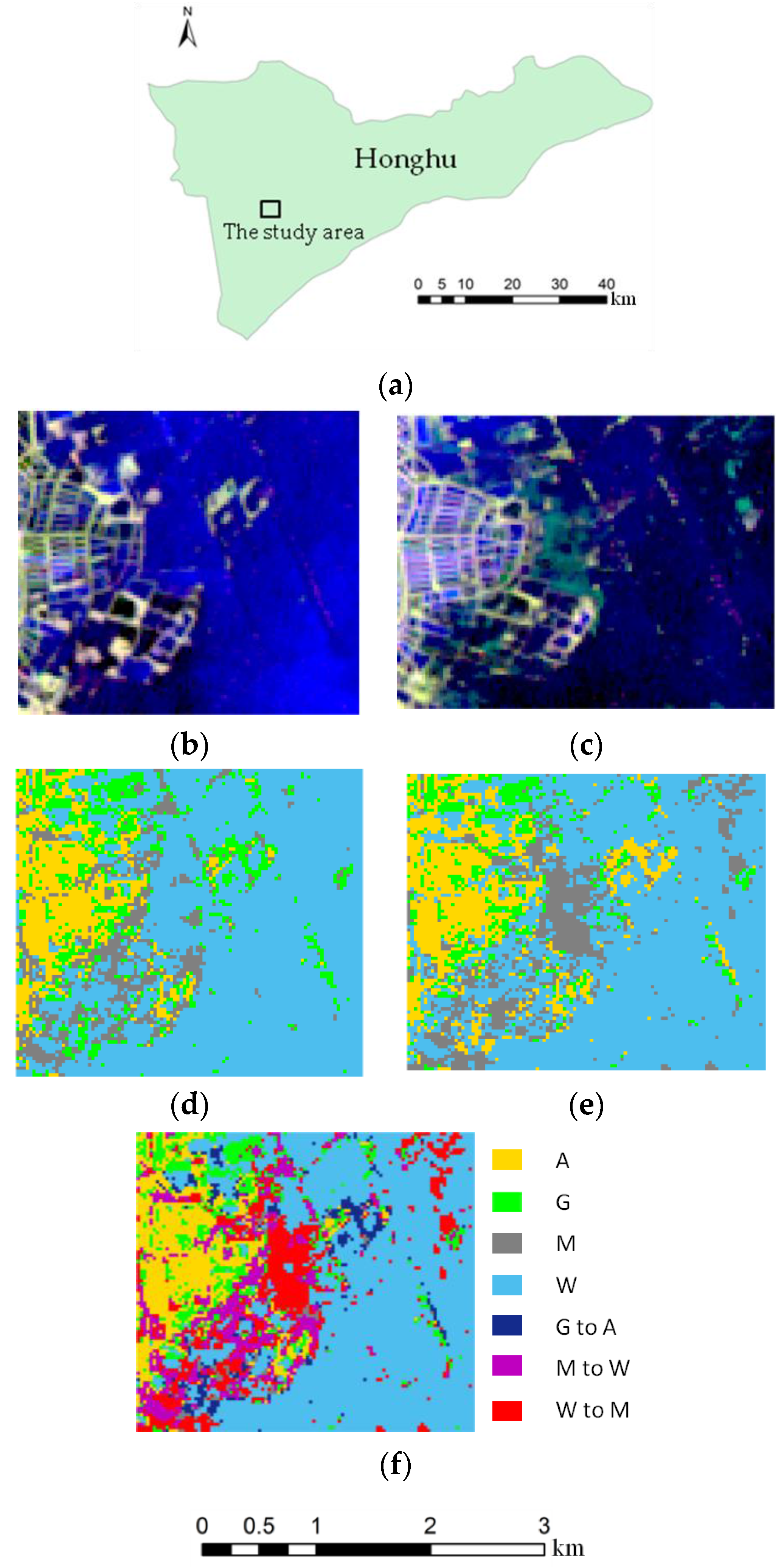
3.1. The Study Area and Datasets

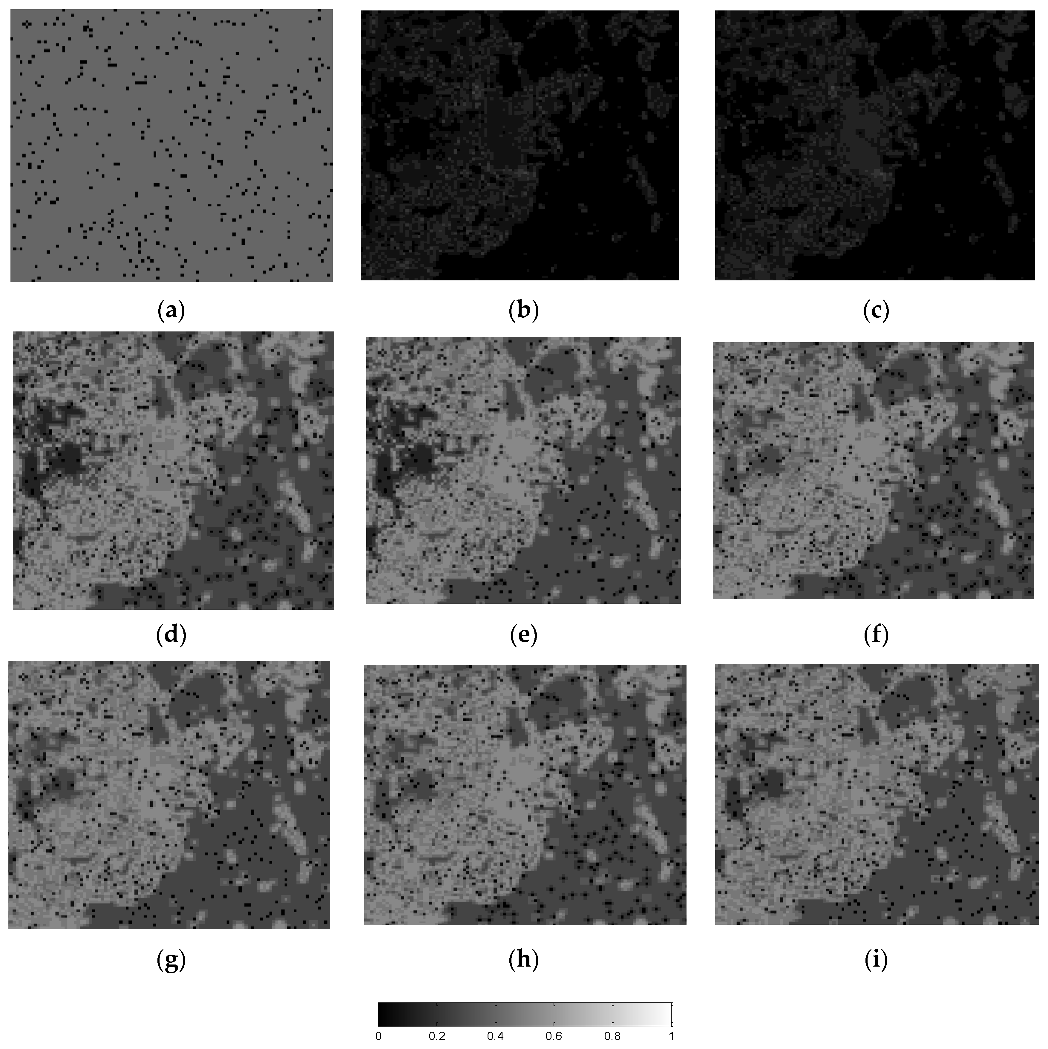
Honghu municipality, Hubei Province, China, which is shown in Figure 1a, is situated in the north of the middle reaches of the Yangtze River and the southeast of the Jianghan Plain. It spans N Latitude ${29}^{\circ }{39}^{\prime }–{30}^{\circ }{12}^{\prime }$ and E Longitude ${113}^{\circ }{07}^{\prime }–{114}^{\circ }{05}^{\prime }$, enjoys a subtropical humid monsoon climate and features lowlands with elevations mostly in the range of 23 m to 28 m above mean sea level. About 30% of its total areas are water bodies comprising a dense network of rivers, streams, lakes and aqueducts (interestingly, both “hu” in “Honghu” and “Hu” in “Hubei” mean lakes in Chinese). Precipitation occurs mostly in the spring and summer, resulting in frequent floods.

Historically, arable land and water bodies are Honghu’s major land resources. From 2011, there was about 40% to 60% less rainfall in the middle and lower reaches of the Yangtze River. Honghu faced the danger of lakes drying up. There were significant changes in land cover types there due to excessive reclamation and cultivation and the situation of more people and less land, such as the transitions from water bodies to mixed land and from natural vegetation (e.g., grasslands) to arable land, suggesting ecological and environmental degradation. With the implementation of lake protection measures by encouraging land reclamation, improving land resources utilization and developing water resources from 2012 through 2015, mixed land cover, which was previously un-used, was gradually restored to water bodies and wetlands. This helped to meet local demands for water resources and restore local ecological environment.

Two sub-scene Landsat ETM+ images of Honghu municipality, flown on 17 May 2012 (Time 1) and 8 August 2013 (Time 2) with Bands 1 to 5 and 7 at 30-m resolution, respectively, were used to derive land cover change information. Composite images for the 2012 and 2013 sub-scene Landsat ETM+ images using Bands 5, 4 and 3 are shown in Figure 1b,c, respectively. The rectangular study area, which is marked in Figure 1a, covers 9964 pixels (94 rows by 106 columns), each of a size of 30 m by 30 m.

Given the aforementioned characteristics of the study area (and land use therein) and the limited spatial resolution of the satellite images employed, for studies of local land cover and its dynamics, we adopted a four-class classification scheme: arable land, grass land, mixed land and water bodies. The mixed land cover type includes abandoned lands and may represent a mixture of all candidate land cover types, which are not easy to discern from satellite image data alone. The type of water bodies includes wetlands and is thus likely a mixture of wetlands with growing habitats and water bodies, per se.

In change detection based on post-classification comparison, images of Times 1 and 2 were classified separately, generating classification maps for Times 1 and 2, as shown in Figure 1d,e, respectively. The classification maps were then compared to create a change map with specific “from-to” change information. A land cover change map with 16 possible combinations of “from-to” change information could be derived for a single-date four-class classification scheme: arable, grass, mixed and water. As there are some non-existing and unlikely change categories, we only kept 7 categories in the final land cover change map, including 4 unchanged or persistent classes and 3 change classes, as shown in Figure 1f.

The 3 change classes shown in Figure 1f are grass land to arable land, mixed land cover to water bodies and water bodies to mixed land cover. Explanations for these changes are: (1) some grasslands changed to arable land because of the increasing demand for agriculture (due to pressure to feed people on limited agricultural land); (2) due to decreased rainfalls during the period, parts of the lakes started to dry out, leading to increased mixed land cover; and (3) ecological restoration led to some restored water bodies from previously-abandoned mixed land.

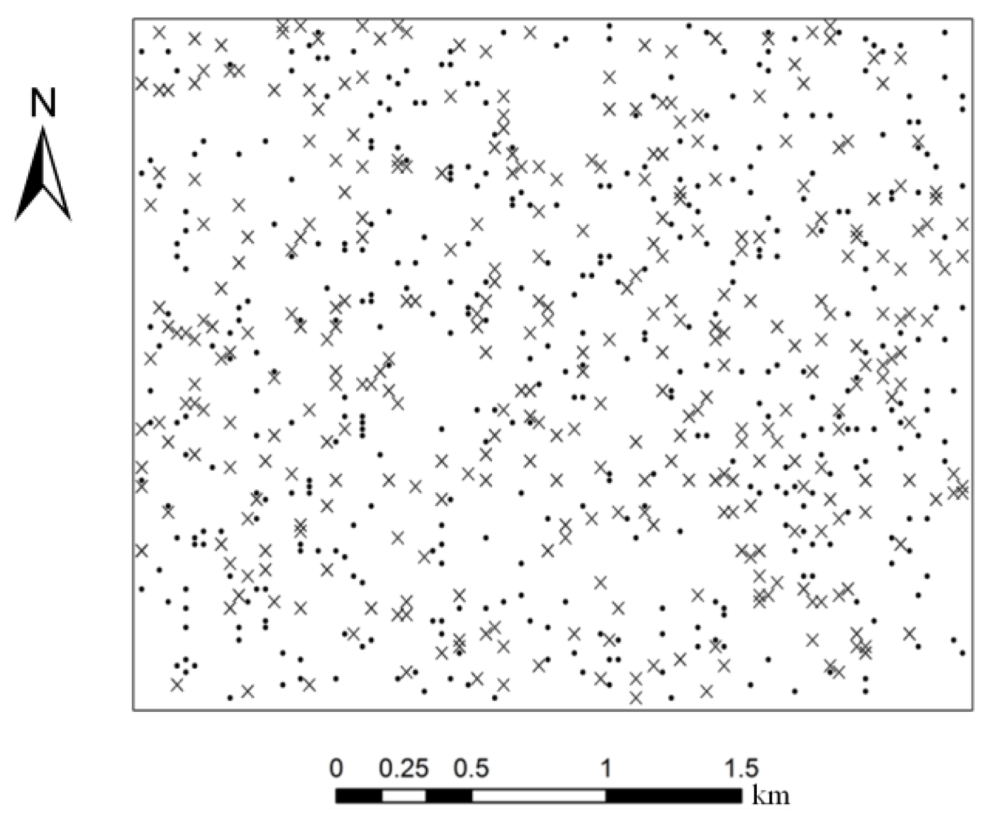
Reference data corresponding to the image data were collected from a combination of field visits and photo-interpretation based on high (spatial) resolution images. Reference cover types for sampled sites in 2013 were ground checked on several dates in October, 2013, while those for 2012 were confirmed using photo-interpretation based on the high-resolution images considered to be in the temporal proximity of the 2012 ETM+ image subset. Photo interpretation was assisted by field surveys and local knowledge to ensure reasonable accuracy in the acquired reference data. The class labeling of all sample locations, whether single-date cover types or bi-temporal change types, were double-checked, with those deleted if the labeling was questionable. Reference data collected were used to determine whether the corresponding pixels on the land cover change map were correctly classified or not.

We should follow statistical principles regarding spatial sampling [28] for collecting references samples, which were used for building models and validating the built models (for local accuracy prediction), respectively. The former set of samples were called training samples, the latter testing samples (which were for the comparison of alternative methods and will be addressed in Section 3.3), in line with the tradition in remote sensing image classification. For collecting both training and testing samples, sampling was carried out using class stratification, with each map class sampled at a fixed proportion or in minimum numbers in the case of minority classes. We set 25 as the minimum number of sample points for minority classes (e.g., the mixed cover type), resulting in 400 and 350 samples for training and testing, respectively. Numbers of samples for individual classes are shown in

Table 1. Numbers of sample pixels for individual land cover change classes.

	Land-Cover Change Detection	Number of Training Samples	Number of Testing Samples	Description
No-change classes	A	48	36	Arable
	G	32	29	Grass
	M	26	21	Mixed
	W	186	179	Water
Change classes	G to A	26	20	Grass to arable
	M to W	37	29	Mixed to water
	W to M	45	36	Water to mixed

, while their distributions are shown in Figure 2.

Testing of the randomness of sample locations was performed based on the “spatial statistic tool” in ArcGIS software system. Using the module of “analyzing patterns”, the Z-test was applied to determine whether the average distance to the nearest neighbors was significantly different from the mean random distance. Z-scores of 0.72 and 0.85 were obtained for the training and testing samples, respectively, which correspond to p-values of 0.46 and 0.39, respectively. Thus, the null hypothesis is accepted that the pattern of the two sets of samples is random at a significance level α = 0.05.

There were a set of 215 extra samples that were used for testing the effectiveness of adaptive sampling by locating a number of further training samples (say 30) according to SEs evaluated at candidate sample locations. This set of 215 samples was set aside, because the so-called adaptive sampling was compared to a random sampling alternative, which requires a larger pool for randomness in sample locations. We will describe this in Section 3.2.

3.2. Results

Based on the training samples, we constructed an error matrix. It was summarized to derive PCC and users’ accuracies for individual classes, as shown in

Table 2. Error matrix for change detection (A: arable, G: grass, M: mixed, W: water, GA: grass to arable, MW: mixed to water, WM: water to mixed). PCC, percent correctly classified.

	A	G	M	W	GA	MW	WM
Users' Accuracy (%)	70.83	71.88	53.85	85.48	57.69	59.46	57.78
PCC (%)	73.25

.

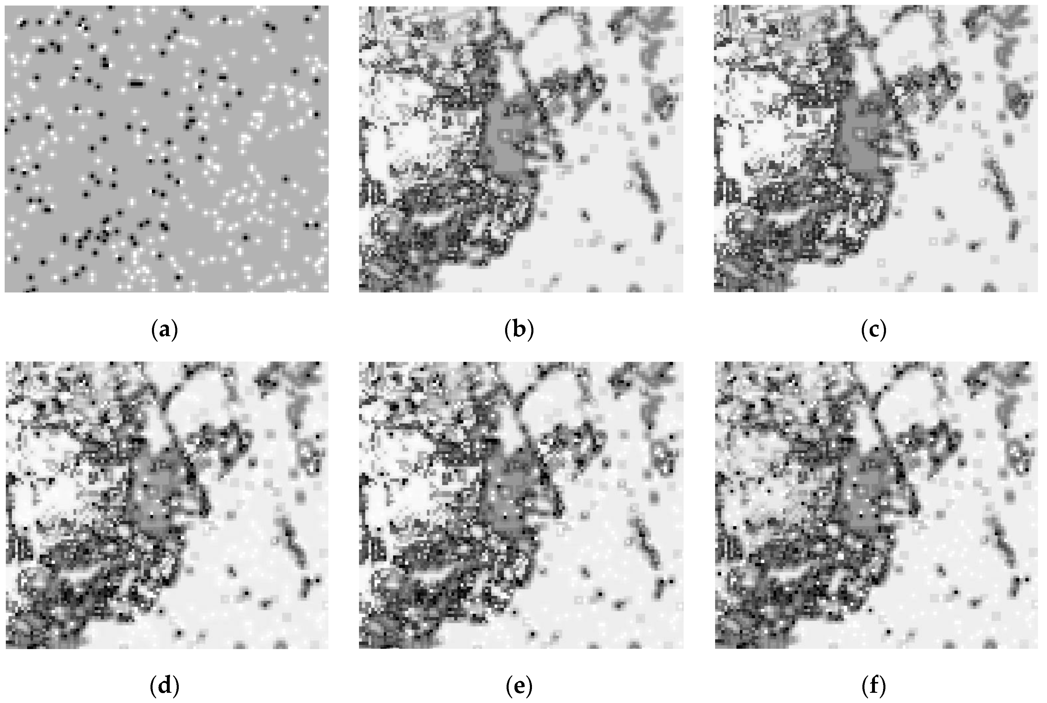
Simple kriging was used to predict the probabilities of correct classification at unsampled locations from training samples. The global mean of RF I indicating classification correctness was assumed to be the PCC measure estimated from training samples, as shown in Table 2. The variogram model for RF I was fitted with indicator data, which coded the (in)correctness in change detection as 1/0. The surface of the probabilities of correct classification at individual pixels is shown in Figure 3a, where it is apparent that predicted probabilities are more similar to sampled values in closer proximity to sampled locations while they appear uniform elsewhere due to the relatively short influence range indicated by the variogram model (fitted with indicator training data) and the nature of simple kriging. As understood, simple kriging predictions will be the known mean value at locations where no sample data are within the specified search radius or where sample data are beyond the influence range. The variogram range was 2 pixels for the datasets here, with the search radius set to equal the range parameter. There were 6967 unsampled locations (i.e., pixels to be predicted), which were beyond the influence range of sample data and, hence, assigned the mean value, which is 73.25%, as shown in Table 1. Consequently, there was a uniform appearance of predicted probabilities at the majority of unsampled locations, as shown in Figure 3a, although local variability in predicted values can be seen clearly by a properly-enlarged version of Figure 3a (or zooming in its softcopy). 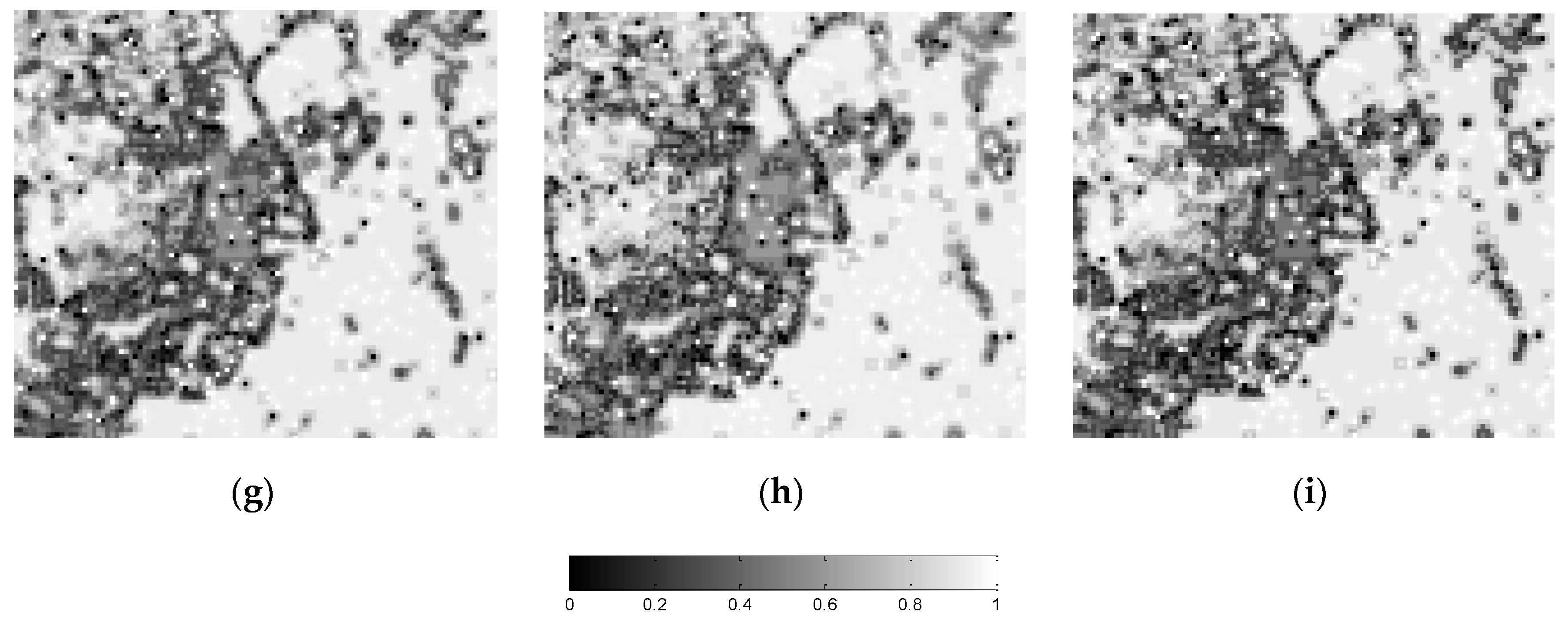Kriging variance was also computed, generating a surface showing SEs (the squared root of kriging variance) at individual locations, as shown in Figure 4a, which depicts the typical appearance of kriging variance: SEs increase with greater distance from sampled locations.

For logistic regression, land cover change class (Class), block contiguity size (L10B), heterogeneity (HET), dominance (DMG) and probability vector of class occurrences in the focal neighborhood (PROB = (p₁(x), p₂(x),…, p₆(x))^T) were used as covariates in different combinations (as shown in

Table 3. Description of models.

Model Number (m)	Model
0	${\mathsf{\beta }}_0$
1a	${\mathsf{\beta }}_0+{\mathsf{\beta }}_{1-6}·Class$
1b	${\mathsf{\beta }}_0+{\mathsf{\beta }}_1·L10B$
1c	${\mathsf{\beta }}_0+{\mathsf{\beta }}_1·HET$
1d	${\mathsf{\beta }}_0+{\mathsf{\beta }}_1·DMG$
1e	${\mathsf{\beta }}_0+{\mathsf{\beta }}_{1-6}·PROB$
2a	${\mathsf{\beta }}_0+{\mathsf{\beta }}_{1-6}·Class+{\mathsf{\beta }}_7·L10B$
2b	${\mathsf{\beta }}_0+{\mathsf{\beta }}_{1-6}·Class+{\mathsf{\beta }}_7·HET$
2c	${\mathsf{\beta }}_0+{\mathsf{\beta }}_{1-6}·Class+{\mathsf{\beta }}_7·DMG$
2d	${\mathsf{\beta }}_0+{\mathsf{\beta }}_{1-6}·Class+{\mathsf{\beta }}_{7-12}·PROB$
3a	${\mathsf{\beta }}_0+{\mathsf{\beta }}_{1-6}·Class+{\mathsf{\beta }}_7·DMG+{\mathsf{\beta }}_8·L10B$
3b	${\mathsf{\beta }}_0+{\mathsf{\beta }}_{1-6}·Class+{\mathsf{\beta }}_7·DMG+{\mathsf{\beta }}_8·HET$
3c	${\mathsf{\beta }}_0+{\mathsf{\beta }}_{1-6}·Class+{\mathsf{\beta }}_7·DMG+{\mathsf{\beta }}_{8-13}·PROB$
4a	${\mathsf{\beta }}_0+{\mathsf{\beta }}_{1-6}·Class+{\mathsf{\beta }}_7·DMG+{\mathsf{\beta }}_{8-13}·PROB+{\mathsf{\beta }}_{14}·L10B$
4b	${\mathsf{\beta }}_0+{\mathsf{\beta }}_{1-6}·Class+{\mathsf{\beta }}_7·DMG+{\mathsf{\beta }}_{8-13}·PROB+{\mathsf{\beta }}_{14}·HET$

) to predict per-pixel probabilities of correct change categorization. Class was coded by 6 binary variables to indicate the presence of one of the 7 classes (as there is one redundancy in the coding of classes). PROB represents the probabilities of individual classes in the focal neighborhood of each pixel (note there is also one redundancy in the probabilities of 7 possible classes as their sum equals 1.0). The models tested are shown in Table 3. Model numbers indicate how many sets of covariates (in addition to the intercept ${\mathsf{\beta }}_0$) are employed for logistic regression: Models 1a to 1e account for the effects of Class, L10B, HET, DMG and PROB on the accuracy of change categorization, respectively; Models 2a to 2d accommodate the effects of L10B, HET, DMG and PROB, respectively, when Class is already taken into account; Models 3a to 3c account for the effects of L10B, HET and PROB, respectively, when Class and DMG are already incorporated; Models 4a and 4b seek to quantify the effects of all L10B and HET, respectively, when Class, DMG and PROB are already included. In other words, the addition of L10B or HET to Model 3c creates Model 4a or 4b, as shown in Table 3.

An exhaustive model selection procedure was applied for finding the model containing the highest number of significant (at α = 0.01) explanatory variables. At each step in the procedure, the significance of the addition of a covariate to a model was tested. The difference between the deviances of two models follows a ${\mathsf{\chi }}_{\text{df}}^2$ distribution, where df is the number of covariates additional to those shared by the two models. A ${\mathsf{\chi }}^2$-test can thus be used to test if adding these df variables to the model significantly improves the fit of the model.

Table 4. Chi-square tests for selected models.

Chi-Square Test (df)	Description: Significance of an Additional Covariate F+1 to a Model Already Containing Variables Fq		Difference in Chi-Square Values	Significance at α = 0.01 Unless Stated Otherwise
	Fq	F+1
D0-D1a (6)	1	Class	88.940	Yes
D0-D1b (1)	1	L10B	74.720	Yes
D0-D1c (1)	1	HET	89.382	Yes
D0-D1d (1)	1	DMG	98.068	Yes
D0-D1e (6)	1	PROB	93.268	Yes
D1a-D2a (1)	1&Class	L10B	19.511	Yes
D1a-D2b (1)	1&Class	HET	28.452	Yes
D1a-D2c (1)	1&Class	DMG	33.511	Yes
D1a-D2d (6)	1&Class	PROB	29.526	Yes
D2d-D3a (1)	1&Class&DMG	L10B	0.548	No
D2d-D3b (1)	1&Class&DMG	HET	0.296	No
D2d-D3c (6)	1&Class&DMG	PROB	11.269	Yes (α = 0.1)
D4a-D3c (1)	1&Class&DMG&PROB	L10B	1.467	No
D4b-D3c (1)	1&Class&DMG&PROB	HET	0.059	No

Dm represents the deviance of model m; models are described in Table 3; F₀ = 1 is multiplied by the intercept ${\mathsf{\beta }}_0$.

shows the significance testing regarding the improvement of the fit of the models by adding an additional covariate (or set of covariates, as for Class and PROB) F₊₁. As shown by Table 4, all of the sets of covariates were significant at $\mathsf{\alpha }$ = 0.01. The impact of local pattern indices (L10B, HET, DMG and PROB) was relatively small, but significant (at $\mathsf{\alpha }$ = 0.01) if the model contained Class, which indicates that part of the impact of these variables was already accounted for by Class. DMG was the most significant at $\mathsf{\alpha }$ = 0.01 if Class were already in the model. Therefore, the analysis was continued with Class and DMG. Adding L10B or HET to a model containing Class and DMG was not significant at α = 0.01. Adding PROB to a model with Class and DMG (Model 3c) was significant at $\mathsf{\alpha }$ = 0.1. Finally, it was tested that adding to Model 3c covariate L10B or HET would not significantly (at α = 0.1 or 0.01) improve the fit. Thus, Model 3c (1&Class&DMG&PROB) was the model containing the highest number of significant covariates.

With Model 3c (1&Class&DMG&PROB) selected using significance testing as above, logistic regression was performed using this model for the pixel-level prediction of classification accuracy. A probability surface was generated assuming spatial independence in binary samples of (in)correct classification, as shown in Figure 3b. Furthermore, SEs in logistic predictions were computed using Equation (15), with the resulting map of SEs shown in Figure 4b.

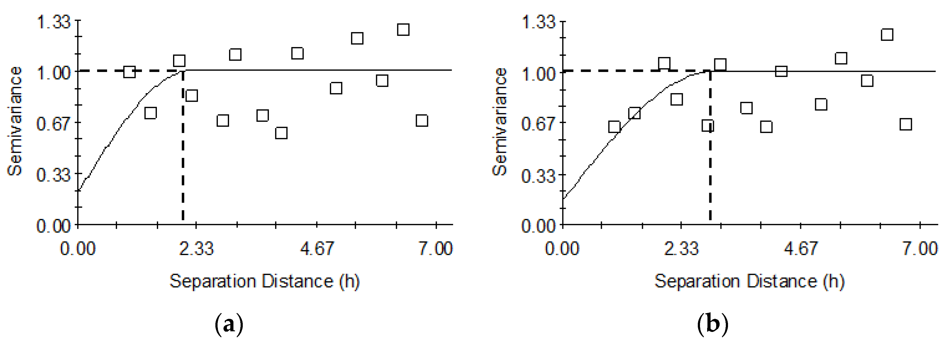
As described in Section 2.3, binary data indicating the (in)correctness in change categorization are often spatially correlated. A challenge in logistic regression involving spatially-correlated binary data is to model spatial dependence in binary response data while estimating regression coefficients β′s. For this, an iterative procedure was undertaken to estimate both logistic model coefficients and variogram parameters via standardized residuals. Upon convergence of the estimates of variogram model parameters and logistic model coefficients, we obtained variogram model parameter values (as shown in

Table 5. Variogram parameters estimated based on standardized residuals of logistic regression.

	Model	Nugget	Sill	Range (pixels)
Initial	Spherical	0.201	1.000	2.210
Final	Spherical	0.156	1.000	2.950

, the final set of parameters values) and logistic model coefficients β′s. β′s were used to predict pixel-level accuracies of change categorization with spatial dependence accommodated. Furthermore, standard errors can be estimated using Equation (15). The predicted accuracies and associated SEs are shown in Figure 3c and Figure 4c, respectively. The differences between the results obtained by logistic regression with spatial correlation accommodated and those without in terms of predicted probabilities and prediction errors are hardly appreciable. The reason is that the range of spatial correlation is just at the scale of about 3 pixels, far less than the average spacings between sampled locations.

After logistic regression, the residuals of logistic regression at sample pixels were used for estimating corrections to regression predictions through simple kriging and then added to the regression predictions (i.e., local means, $\widehat{\mathsf{\pi }}\left(x\right)$) to obtain the corrected probabilistic measures of classification accuracies for individual pixels. Equations (21) and (22) were the formulas applied for computing the corrected probabilities of correct classification and the corresponding standard errors, respectively. For kriging of regression residuals, two approaches were implemented: one without consideration for spatial correlation in logistic regression (Table 5, the initial set of variogram parameter values) and the other with consideration for spatial correlation therein, as shown in Section 2.3 (see Table 5, the final set of variogram parameter values as mentioned previously). To aid the interpretation of the results, Figure 5a shows variogram model parameters with no spatial correlation incorporated in logistic regression (corresponding to the initial set of parameters in Table 5), while Figure 5b shows variogram model parameters fitted iteratively with those of logistic regression where spatial correlation was considered (pertaining to the final set of parameters in Table 5). The sills shown in Figure 5a,b, which are the sum of nugget and structural variances, were set to 1.0 because standardized residuals were used to compute experimental variograms. Results with the former were meant to provide a baseline for the latter, which is computationally more expensive due to the iteration involved in parameter estimation and variogram modeling.

For the former, the map depicting corrected probabilities of correct change categorization and the SEs in the corrected probabilistic measures are shown in Figure 3d and Figure 4d, respectively. For the latter, the maps depicting corrected probabilities and their SEs are shown in Figure 3e and Figure 4e, respectively. Unsurprisingly, the results shown in pairs (i.e., Figure 3b,c and Figure 3d,e) indicate no apparent differences. This visual interpretation will be supported with testing results in the next subsection.

Having undertaken experiments about significant covariates for logistic regression and the advantages of logistic-regression-kriging (with or without full treatment of spatial correlation in the estimation of variogram model parameters and regression coefficients) against regression or kriging alone, we turn to the effects of adaptive sampling guided by uncertainty measures (i.e., SEs) in current local accuracy predictions (based on existing training sample data). To test the effectiveness of adaptive sampling (it is labeled so because further samples are selected according to SEs in existing accuracy predictions), we used the pool of the extra 215 samples as the population to get some further training samples. Adaptive sampling was actually undertaken based on the results obtained by logistic-regression-kriging with or without fuller treatment of spatial correlation. We selected 30 further training samples, whose SEs were significantly larger than the rest in the set of 215 samples. For comparison with adaptive sampling pursued here, we also applied stratified random sampling (regardless of SEs) based on the same pool of extra 215 samples to get 30 random training samples. Two sampling approaches and two sets of prior logistic-regression-kriging results gave rises to four more sets of results. These four prediction results are shown in Figure 3f to Figure 3i, while their corresponding maps of SEs are shown in Figure 4f to Figure 4i. Clearly, SEs shown in Figure 4f,g and Figure 4h,i indicate a slight decrease as compared to those shown in Figure 4d,e, respectively.

3.3. Testing

The performance of the nine different methods described previously for accuracy prediction can be evaluated by comparing predicted values $\widehat{p}\left(x_j\right)$ with actual observations $i\left(x_j\right)$ at 350 testing sample locations using the following four measure: mean error (ME), mean absolute error (MAE), root mean square error (RMSE) and sums-of-squares ($R_{SS}^2$). They are computed as follows:

$$ME=\frac{1}{n_t}{\displaystyle \sum }_{j=1}^{n_t}\left[i\left(x_j\right)-\widehat{p}\left(x_j\right)\right]$$

(23)

$$MAE=\frac{1}{n_t}{\displaystyle \sum }_{j=1}^{n_t}\left|i\left(x_j\right)-\widehat{p}\left(x_j\right)\right|$$

(24)

$$RMSE=\sqrt{\frac{1}{n_t}{\displaystyle \sum }_{j=1}^{n_t}{\left[i\left(x_j\right)-\widehat{p}\left(x_j\right)\right]}^2}$$

(25)

$$R_{SS}^2=1-\frac{{\sum }_{j=1}^{n_t}{\left[i\left(x_j\right)-\widehat{p}\left(x_j\right)\right]}^2}{{\left(i\left(x_j\right)-\overline{p}\right)}^2}$$

(26)

where n_t is the number of testing samples and $\overline{p}$ is the mean of observed values. As recommended in the literature, $R_{SS}^2$ measures the proportion of explained variation by logistic regression [29]. As the predictions of probabilities of (in)correct classification can be transformed to indicator data at the threshold of 0.5, we can also compute measures of PCCs to assess the accuracy of predictions. These measures were computed for the nine prediction methods, as presented in

Table 6. Comparison of methods for predicting classification accuracy.

	PCC (%)	ME	MAE	RMSE	${\mathit{R}}_{SS}^{\mathbf{2}}$
Null model	58.86	−0.111	0.465	0.505	−0.051
Indicator kriging	60.86	−0.107	0.454	0.496	−0.018
Logistic regression
no spatial correlation considered	69.71	−0.146	0.341	0.441	0.200
spatial correlation considered	70.29	−0.146	0.340	0.440	0.201
Logistic regression and kriging of residuals
no spatial correlation considered in regression	70.57	−0.146	0.338	0.439	0.202
spatial correlation considered in regression	71.14	−0.135	0.335	0.437	0.211
Logistic regression and kriging of residuals (with extra training samples)
no spatial correlation considered in regression
Random sampling	72.29	−0.127	0.328	0.422	0.266
Adaptive sampling	76.00	−0.104	0.318	0.403	0.331
spatial correlation considered in regression
Random sampling	72.57	−0.124	0.327	0.421	0.269
Adaptive sampling	77.43	−0.080	0.318	0.402	0.332

. The results for the null model, which assigns 73.25% (the PCC estimate from Table 2) as the prediction of accuracy for all pixels, are used as the baseline for the methods shown in Table 6.

As seen from Table 6, all methods register negative ME values (i.e., ME < 0). This suggested that all of the methods of prediction used here over-estimated accuracy in change categorization (as observed values < predicted values). Because of unbiasedness in kriging, the ME value of predictions by indicator kriging is the closest to 0.

As indicated by Table 6, there is a tendency of better performances, as demonstrated by decreasing MAEs and RMSEs, but increasing PCCs and $R_{SS}^2$ for methods shown top down in the rows in Table 6. In particular, as shown in Table 6, indicator kriging is the worst at predicting local accuracies, while logistic-regression-kriging accommodating spatial correlation was the best. Note that the null model, which sets a baseline for all other methods tested, was worse than any of the other methods tested, as shown in Table 6.

However, there are only modest gains in accuracy achieved by logistic-regression-kriging accommodating spatial correlation as opposed to the alternative implementation without considering spatial correlation. This is also true of logistic regression with spatial correlation considered as opposed to that without. The trade-off between computation cost and accuracy gain in prediction accuracy is thus important. Map users must decide whether the extra cost involved in regression-kriging is justifiable with the modest gains in prediction accuracy.

It should be noted that adequate reference samples are always important for ensuring reasonable accuracy in predictions (about local classification accuracies) by the methods tested here regardless of their sophistication. Given a specific sample size, the sample design will be important for optimum predictions. As mentioned previously, SEs maps shown in Figure 4 could be used to locate densification training samples to facilitate the developments of sampling strategies for accurate yet efficient characterization of classification accuracy, as ground sampling is often expensive. We tested the results (shown in subfigures (f) to (i)) obtained by adding extra training samples (adaptive and random modes), using the same testing samples. The testing statistics are listed in Table 6’s lower block of rows regarding the effects of extra training samples. They indicate that adaptive sampling for extra training samples is more cost-effective than random sampling. For instance, for the case of combined logistic-regression-kriging with the treatment of spatial correlation in regression, 7.5% more training samples led to about 8.8% and 57.3% increases in prediction accuracy, as measured by PCCs and $R_{SS}^2$, respectively. In comparison, for random sampling, the same increase in training sample size led to only about 2.0% and 27.5% increases in prediction accuracy, as measured by PCCs and $R_{SS}^2$, respectively The relationships between uncertainty-informed adaptive sampling and prediction performances should be studied further, although this is beyond the scope of this paper.

3.4. Discussion

The proposed methods for mapping local accuracies in land cover change maps can be usefully explored in combination with work on landscape dynamics monitoring and modelling, such as that described by Millington et al. [1] and Rutherford et al. [2], and related research efforts [28,30,31,32]. Firstly, results from maps of predicted changes using methods developed in [1,2] may well be evaluated with respect to their local accuracies by using the methods proposed in this paper. This would provide useful information about local variations of accuracies in predicted changes, which would in turn be valuable for improving model performances. Secondly, the accuracies of the predicted change maps using models developed in [1,2] are subject not only to model performances, but also accuracies of the input datasets that are used as covariates in modeling. If other categorical maps are included as covariate map layers, it is possible to apply the methods proposed in this paper to quantify their local accuracies, which can be used along with information about accuracies in other types of input maps to analyze inaccuracies from the input, through the modeling process, to the output. Thirdly, inaccuracies in reference data are yet another dimension of the accuracy issues raised here in this paper and in related literature, such as Wickham et al. [30]. Reference data imperfection should be examined so that we have a clearer picture of inaccuracies in the gathering and processing of land cover information and in the broader context of landscape dynamics modeling. Fourthly, the issue of scale raised in the literature, such as Millington et al. [1], Zhang et al. [15] and Pontius et al. [31], should be considered for further developments of the methods proposed here in this paper, given that the proposed methods are designed to work on the local scale (focal to be exact) and may not be linearly translatable to coarser scales, as discussed previously in Section 2.2. Fifthly, we should be aware of the limitations of single-date map comparisons between years, as pointed by Bontemps et al. [32], and promote time series analysis in landscape change monitoring and dynamics modelling, seeking to account for temporal dependence and phenology in data analysis and modeling. Lastly, sampling design [28] remains essential for accuracy characterization, especially for change analysis and dynamics modeling, no matter how sophisticated the methods for regression, kriging and others become. The adaptive sampling strategy preliminarily developed and tested in this paper should be explored further for large-scale problem-solving and in operational settings.

The methods tested in this paper are suitable for predicting local classification accuracies, which, however, cannot be directly used for computing accuracies in derivative products or analyses, such as those for landscape ecology, unless we are willing to assume independence among RVs representing classification (in)correctness at individual locations. To accommodate the spatial dependence existing among these RVs, geostatistical simulation should be applied [33]. For instance, simulation approaches are needed for: (1) the determination of local accuracies in coarsened and object-based [34] land cover change maps based on maps of finer resolution, as neighboring pixels in fine-resolution maps are likely spatially correlated in terms of misclassification; (2) the rigorous quantification of SEs in predicted local accuracies, especially when normality cannot be assumed for the small samples of binary data; (3) the error propagation in area estimates that are likely to involve counting numbers of pixels belonging to certain classes, where pixels close by cannot be assumed independent; and (4) the other ecological modeling and application scenarios where land cover change maps are part of the input data. These will form topics for further research.

4. Conclusions

This paper has focused on situations where users of land cover change maps would like to evaluate such maps’ local accuracies based on some validation (training) samples and by exploiting the association between the occurrences of (in)correct classifications and local patterns of class occurrences in the map being assessed. Experiments with empirical data showed that combined logistic regression and residual kriging is the most accurate in terms of conventional error measures and R-squared measures (adapted for binary data), indicating the proportions of variation explained by alternative accuracy predicators. It was also found that more efficiency in predictions can be obtained by not considering spatial correlation in regression (thus, no need for iterative estimation of regression coefficients and variogram parameters) without significantly compromising accuracy in prediction, especially when variogram models suggest relatively weak spatial dependence in the observed data concerning (in)correct classifications. The SEs evaluated along with accuracy predictions can be used to guide the locating of further training samples to improve the predictions of local accuracies while enhancing sampling efficiency, contributing to adaptive and progressive sampling designs for accuracy characterization. Furthermore, the sampling strategy preliminarily explored in this paper may be usefully extended to provide feedbacks and diagnosis about information products quality, for example by identifying locations of low predicted accuracies and suggesting ways for improving classification accuracies, especially for classes or locations of high priorities in terms of environmental analysis and applications.

Although the methods were designed and tested from users’ perspectives, land cover change map producers may also implement the proposed methods for evaluating their map products’ local accuracies. Obviously, covariates for logistic regression will be different, as producers are more solvable in terms of access to source data employed and relevant metadata. For them, richness in source data and more information about map production processes are likely to lead to more detailed and accurate predictions of map accuracies, although this remains to be tested.

References

1. Millington, J.D.; Perry, G.L.; Romero-Calcerrada, R. Regression techniques for examining land use/cover change: A case study of a Mediterranean landscape. Ecosystems 2007, 10, 562–578. [Google Scholar] [CrossRef]
2. Rutherford, G.N.; Bebi, P.; Edwards, P.J.; Zimmermann, N.E. Assessing land-use statistics to model land cover change in a mountainous landscape in the European Alps. Ecol. Model. 2008, 212, 460–471. [Google Scholar] [CrossRef]
3. Wu, J.; Zhang, Q.; Li, A.; Liang, C. Historical landscape dynamics of Inner Mongolia: Patterns, drivers, and impacts. Landsc. Ecol. 2015, 30, 1–20. [Google Scholar] [CrossRef]
4. Fuller, R.; Smith, G.; Devereux, B. The characterisation and measurement of land cover change through remote sensing: Problems in operational applications? Int. J. Appl. Earth Observ. Geoinf. 2003, 4, 243–253. [Google Scholar] [CrossRef]
5. Chen, J.; Chen, J.; Liao, A.; Cao, X.; Chen, L.; Chen, X.; He, C.; Han, G.; Peng, S.; Lu, M. Global land cover mapping at 30 m resolution: A POK-based operational approach. ISPRS J.Photogramm. Remote Sens. 2014, 103, 7–27. [Google Scholar] [CrossRef]
6. Goodchild, M.; Zhang, J.; Kyriakidis, P. Discriminant models of uncertainty in nominal fields. Trans. GIS 2009, 13, 7–23. [Google Scholar] [CrossRef]
7. Lechner, A.M.; Langford, W.T.; Bekessy, S.A.; Jones, S.D. Are landscape ecologists addressing uncertainty in their remote sensing data? Landsc. Ecol. 2012, 27, 1249–1261. [Google Scholar] [CrossRef]
8. Congalton, R.; Gu, J.; Yadav, K.; Thenkabail, P.; Ozdogan, M. Global land cover mapping: A review and uncertainty analysis. Remote Sens. 2014, 6, 12070–12093. [Google Scholar] [CrossRef]
9. Olofsson, P.; Foody, G.M.; Herold, M.; Stehman, S.V.; Woodcock, C.E.; Wulder, M.A. Good practices for estimating area and assessing accuracy of land change. Remote Sens. Environ. 2014, 148, 42–57. [Google Scholar] [CrossRef]
10. Burrough, P.A.; Frank, A.U. Geographic Objects with Indeterminate Boundaries; Taylor & Francis: London, UK, 1997. [Google Scholar]
11. Wickham, J.D.; Stehman, S.V.; Gass, L.; Dewitz, J.; Fry, J.A.; Wade, T.G. Accuracy assessment of NLCD 2006 land cover and impervious surface. Remote Sens. Environ. 2013, 130, 294–304. [Google Scholar] [CrossRef]
12. Foody, G.M. Local characterization of thematic classification accuracy through spatially constrained confusion matrices. Int. J. Remote Sens. 2005, 26, 1217–1228. [Google Scholar] [CrossRef]
13. Khorram, S. Accuracy Assessment of Remote Sensing-Derived Change Detection; American Society for Photogrammetry and Remote Sensing: Bethesda, MD, USA, 1999. [Google Scholar]
14. Steele, B.M. Maximum posterior probability estimators of map accuracy. Remote Sens. Environ. 2005, 99, 254–270. [Google Scholar] [CrossRef]
15. Zhang, J.; Atkinson, P.M.; Goodchild, M.F. Scale in Spatial Information and Analysis; CRC Press: Boca Raton, FL, USA, 2014. [Google Scholar]
16. Steele, B.M.; Winne, J.C.; Redmond, R.L. Estimation and mapping of misclassification probabilities for thematic land cover maps. Remote Sens. Environ. 1998, 66, 192–202. [Google Scholar]
17. Smith, J.H.; Stehman, S.V.; Wickham, J.D. Impacts of patch size and land-cover heterogeneity on thematic image classification accuracy. Photogramm. Eng. Remote Sens. 2002, 68, 65–70. [Google Scholar]
18. Smith, J.H.; Stehman, S.V.; Wickham, J.D.; Yang, L. Effects of landscape characteristics on land-cover class accuracy. Remote Sens. Environ. 2003, 84, 342–349. [Google Scholar] [CrossRef]
19. Oort, P.A.J.v.; Bregt, A.K.; Bruin, S.d.; Wit, A.J.W.d.; Stein, A. Spatial variability in classification accuracy of agricultural crops in the Dutch national land-cover database. Int. J. Geogr. Inf. Sci. 2004, 18, 611–626. [Google Scholar] [CrossRef]
20. Burnicki, A.C. Modeling the probability of misclassification in a map of land cover change. Photogramm. Eng. Remote Sens. 2011, 77, 39–49. [Google Scholar] [CrossRef]
21. Journel, A.G. Nonparametric estimation of spatial distributions. J. Int. Assoc. Math. Geol. 1983, 15, 445–468. [Google Scholar] [CrossRef]
22. Hengl, T.; Heuvelink, G.B.M.; Stein, A. A generic framework for spatial prediction of soil variables based on regression-kriging. Geoderma 2004, 120, 75–93. [Google Scholar] [CrossRef]
23. Agresti, A. Categorical Data Analysis, 2nd ed.; John Wiley & Sons, Inc.: Hoboken, NJ, USA, 2002. [Google Scholar]
24. Gotway, C.A.; Stroup, W.W. A Generalized linear model approach to spatial data analysis and prediction. J. Agric. Biol. Environ. Stat. 1997, 2, 157–178. [Google Scholar] [CrossRef]
25. Pebesma, E.J.; Duin, R.N.M.; Burrough, P.A. Mapping sea bird densities over the North Sea: Spatially aggregated estimates and temporal changes. Acta Obstet. Et Gynecol. Scand. 2005, 16, 573–587. [Google Scholar] [CrossRef]
26. Liang, K.; Zeger, S.L. Longitudinal data analysis using generalized linear models. Biometrika 1986, 73, 13–22. [Google Scholar] [CrossRef]
27. Albert, P.S.; Mcshane, L.M. A generalized estimating equations approach for spatially correlated binary data: Applications to the analysis of neuroimaging data. Biometrics 1995, 51, 627–638. [Google Scholar] [CrossRef] [PubMed]
28. Stehman, S.V. Impact of sample size allocation when using stratified random sampling to estimate accuracy and area of land-cover change. Remote Sens. Lett. 2012, 3, 111–120. [Google Scholar] [CrossRef]
29. Mittlböck, M.; Schemper, M. Computing measures of explained variation for logistic regression models. Comput. Methods Programs Biomed. 1998, 58, 17–24. [Google Scholar] [CrossRef]
30. Wickham, J.D.; Stehman, S.V.; Fry, J.A.; Smith, J.H.; Homer, C.G. Thematic accuracy of the NLCD 2001 land cover for the conterminous United States. Remote Sens. Environ. 2010, 114, 1286–1296. [Google Scholar] [CrossRef]
31. Pontius, R.G.; Huffaker, D.; Denman, K. Useful techniques of validation for spatially explicit land-change models. Ecol. Model. 2004, 179, 445–461. [Google Scholar] [CrossRef]
32. Bontemps, S.; Bogaert, P.; Titeux, N.; Defourny, P. An object-based change detection method accounting for temporal dependences in time series with medium to coarse spatial resolution. Remote Sens. Environ. 2008, 112, 3181–3191. [Google Scholar] [CrossRef]
33. Kyriakidis, P.C.; Dungan, J.L. A geostatistical approach for mapping thematic classification accuracy and evaluating the impact of inaccurate spatial data on ecological model predictions. Environ. Ecol. Stat. 2001, 8, 311–330. [Google Scholar] [CrossRef]
34. Radoux, J.; Bogaert, P.; Fasbender, D.; Defourny, P. Thematic accuracy assessment of geographic object-based image classification. Int. J. Geogr. Inf. Sci. 2011, 25, 895–911. [Google Scholar] [CrossRef]
Figure 1. The study area, the images used and the maps derived: (a) the study area; (b,c) sub-scene Landsat ETM+ images for 2012 and 2013, respectively; (d,e) land cover classification maps showing 4 classes of land cover for 2012 and 2013, respectively; and (f) land cover change map derived from the bi-temporal image data, showing 7 classes including 4 unchanged and 3 changed classes. In (d,e,f), A, G, M and W indicate arable land, grass land, mixed land cover and water bodies, respectively.
Ijgi 05 00113 g001
Figure 2. Locations of training (400) and testing (350) samples (∙, training samples; ×, testing samples).
Ijgi 05 00113 g002
Figure 3. The probability maps generated by different methods: (a) indicator kriging; (b,c) logistic regression, without and with spatial correlation considered, respectively; (d,e) logistic regression and kriging, without and with spatial correlation considered in regression, respectively; (f,g) logistic regression (without considering spatial correlation) and kriging, with extra training samples collected by random and adaptive sampling, respectively; (h,i) logistic regression (considering spatial correlation) and kriging, with extra training samples collected by random and adaptive sampling, respectively.
Ijgi 05 00113 g003aIjgi 05 00113 g003b
Figure 4. Maps of prediction standard errors for different methods (the same set of methods as listed in Figure 3): (a) indicator kriging; (b,c) logistic regression, without and with spatial correlation considered, respectively; (d,e) logistic regression and kriging, without and with spatial correlation considered in regression, respectively; (f,g) logistic regression (without considering spatial correlation) and kriging, with extra training samples collected by random and adaptive sampling, respectively; (h,i) logistic regression (considering spatial correlation) and kriging, with extra training samples collected by random and adaptive sampling, respectively.
Ijgi 05 00113 g004
Figure 5. Experimental variograms (shown as small squares) and their fitted models (shown as curves) based on the standardized residuals when: (a) no spatial correlation is considered in logistic regression; and (b) considering spatial correlation in logistic regression; (a,b) corresponding to the initial and final set of parameters in Table 5, respectively.
Ijgi 05 00113 g005