A Point-Set-Based Footprint Model and Spatial Ranking Method for Geographic Information Retrieval

Abstract

In the recent big data era, massive spatial related data are continuously generated and scrambled from various sources. Acquiring accurate geographic information is also urgently demanded. How to accurately retrieve desired geographic information has become the prominent issue, needing to be resolved in high priority. The key technologies in geographic information retrieval are modeling document footprints and ranking documents based on their similarity evaluation. The traditional spatial similarity evaluation methods are mainly performed using a MBR (Minimum Bounding Rectangle) footprint model. However, due to its nature of simplification and roughness, the results of traditional methods tend to be isotropic and space-redundant. In this paper, a new model that constructs the footprints in the form of point-sets is presented. The point-set-based footprint coincides the nature of place names in web pages, so it is redundancy-free, consistent, accurate, and anisotropic to describe the spatial extents of documents, and can handle multi-scale geographic information. The corresponding spatial ranking method is also presented based on the point-set-based model. The new similarity evaluation algorithm of this method firstly measures multiple distances for the spatial proximity across different scales, and then combines the frequency of place names to improve the accuracy and precision. The experimental results show that the proposed method outperforms the traditional methods with higher accuracies under different searching scenarios.

1. Introduction

In the recent big data era, the rapid development of Web and location-based technologies, as well as the widespread applications of social media tagged with location info, has contributed to the diversity and magnanimity of geographic data, along with the urgent demand of acquiring the accurate geographic information. It is reported that 20% of searches on Google are related to locations [1]. An annual report from comScore/TMPDM that referred to local search behavior in 2013 also stated that by the year 2013, there were nearly 86 million people in the United States seeking local business information on their mobile devices, a 63% increase since 2010 [2]. All of these figures illustrate that geographic information is pervasive on the web and geographic entities are frequent in user queries. The acquisition and processing of geographic information, especially geographic information retrieval, is of crucial study value and a promising application prospect.

First proposed by Larson [3], geographic information retrieval (GIR) is defined as a process concerned with providing access to geo-referenced information sources. GIR includes all of the areas that have traditionally formed the core of information retrieval (IR) research, with an emphasis, or addition, of spatially- and geographically oriented indexing and retrieval.

The main research areas of GIR are generalized into seven challenges by Jones [4]: detecting, disambiguating, interpreting, indexing, ranking, designing user interfaces, and evaluating. Because of the multiple sources and media types of geographic data, the information implied is always obscure. This leads to diverse forms of footprints, which determine the spatial ranking algorithms. Peters et al. [5] built the footprints of documents with place names and compared the syntactic differences between phrases to assess similarities. However, the evaluation of spatial similarity is based on semantics: two different phrases that suggest the same spatial area are considered to be one place name. In this case, the criterion of similarity is no longer literal, but rather the implied “proximity” of the entities.

To satisfy the geographic semantics, some researchers [6,7,8] have denoted the footprints as MBRs (Minimum Bounding Rectangular) or convex hulls that contain the space that the place names in the documents refer to, and the spatial similarity assessment for ranking depends on the topological relationship between two polygons, regular or irregular [9]. According to GeoCLEF, a cross-language geographic retrieval track of the Cross Language Evaluation Forum (CLEF) that aims to evaluate GIR systems for spatial and multilingual searching tasks [10,11], MBR and convex hull are the most commonly used models at present. However, the convex hull model is not as pervasive as the MBR model due to the complexity of the convex hull model. Generating and storing the convex hull of a document, as well as computing the topological relationship between convex hulls, is time- and space-consuming.

Although the polygon models are simple and straightforward, both MBRs and convex hulls suffer from inherent defects that derive from the nature of polygons and topology evaluation. The specific disadvantages of the aforementioned models are as follows:

(a)

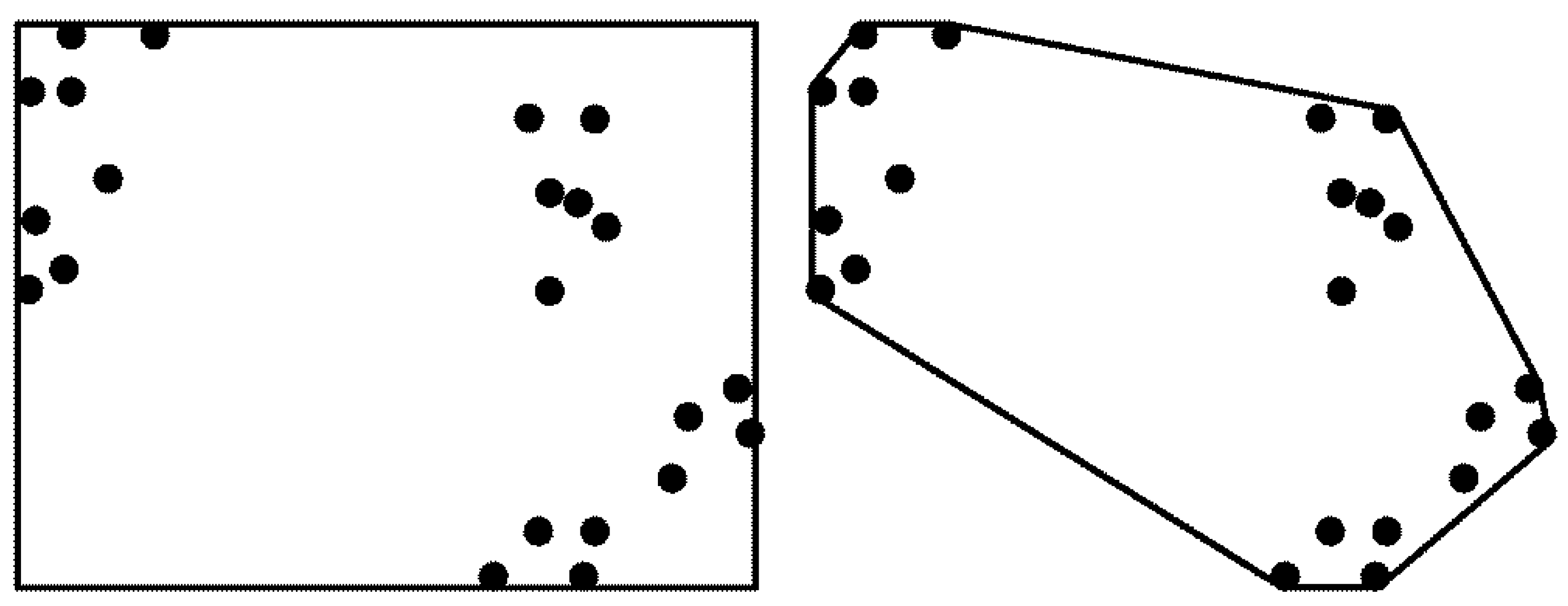
Space redundancy. The most obvious weakness happens when polygon models represent diagonal, irregular, non-convex, or multi-part regions [12]. The polygons will cover more space than the documents refer to (Figure 1), and if the query falls in the redundant space, irrelevant documents will be retrieved.

(b)

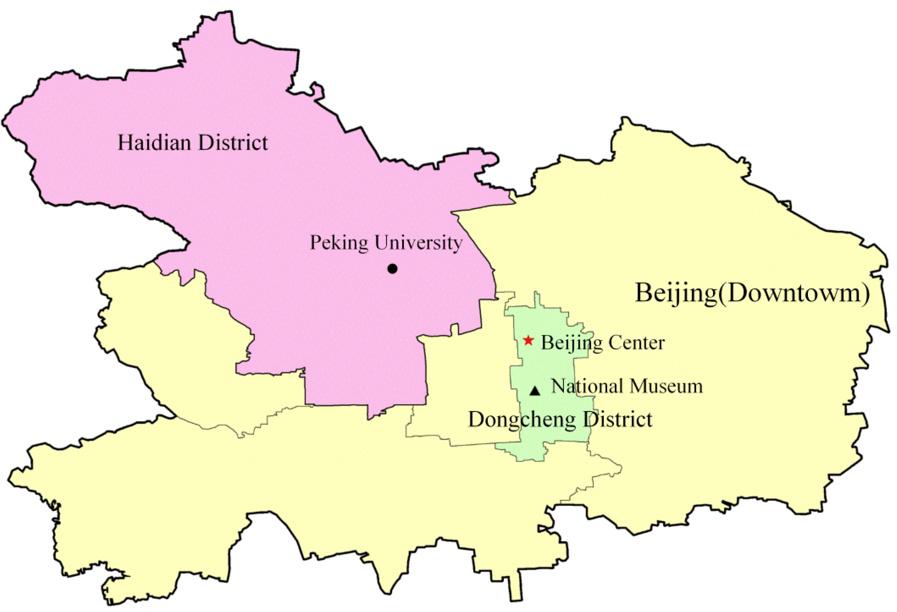
Location swamping. The documents may contain locations on different scales, e.g., Beijing, Haidian District, and Peking University (Figure 2). However, the final polygon only represents the overall area, and inner locations will be masked, which will lead to information loss. For example, if the query is Peking University, and there are two documents both referring to Beijing, but one document mentions Peking University and the other does not, then the polygon model will be unable to discriminate between these two documents and fail to target the most relevant document, because the footprint of these two documents are presented as the same polygon.

(c)

Inaccuracy. The similarity evaluation based on polygon models is to examine the topological relationship, i.e., whether they touch/intersect/contain each other or not. Because this relationship is binary (0 for separation and 1 for intersection), the result is rough. This evaluation method does not discriminate the cognition of “far” or “near”, which is important with regard to spatial cognition of human beings, and the distance between two entities should be stressed. Some improvements have been made to conquer the inaccuracy of binary evaluation by examining the proximity in three scenarios: contain, overlap, and proximity [11]. Correspondingly, the evaluation function is adjusted from binary to an area ratio, which will improve the accuracy, but the result may not always conform to common sense. For example, if the query is “Beijing” and we retrieve this query from two documents, A and B, and the footprint of document A is “Dongcheng District” and the footprint of document B is “Haidian District” (Figure 2). Then when using the evaluation function of area ratio, document B will rank higher than A because the area of Haidian District is larger than the area of Dongcheng District. However, because document A and document B both refer to sub-regions of Beijing and there is no more information to discriminate the relevance, when retrieving Beijing, both sub-regions should rank the same.

(d)

Homogeneity. The space within a single MBR is considered equally, even though some of the places may be more important due to higher frequencies. For example, if one document mentions Haidian district 50 times, and the other document mentions Haidian district only once, then the polygon footprints for these two documents may be the same. However, in traditional text retrieval, according to the TF-IDF model [13], the entities with higher frequency tend to have higher ranking scores. Similarly, we consider the first document to be definitely more related to Haidian district than the second document, because the first document mentions the place more often.

Some efforts have been made to overcome the above issues. Improved geometric footprint models, including multiple polygons [14,15] and MBR set [16,17], are presented as one kind of solutions. De Andrade [18] further integrates the overlap degree of MBRs with the spatial relevance, which is defined by the overlapping frequencies of MBRs, to calculate the spatial rankings. De Sabbata and Reichenbacher [19,20] present five fine-grained criteria (including topicality, spatiotemporal proximity, directionality, cluster, and colocation) for calculating spatial relevance score. Although these methods avoid the redundancy problem, issues about location swamping and homogeneity still exist. Semantically rich models are also presented as the solutions to such issues. Sets of place names are firstly used to represent the document extents and the relevance is calculated by their hierarchical relationships [21,22]. Furthermore, geographic ontologies or knowledge graphs, instead of footprints, are constructed to measure the semantic similarities for spatial rankings [23,24,25,26]. The latest topic models are also utilized in geographic information retrieval to find the similar place-related documents based on latent semantics [23,27]. Although these semantic-based methods can integrate spatial and thematic relevance together to rank, ontologies and knowledge are domain-specific and usually difficult to be constructed. Compared with spatial distance, semantic distance may lead to inaccuracy and missing information. In recent years, crowdsourcing, social networks, and other big data resources are incorporated into semantic and geometric footprint models for spatial proximity and ranking calculations [28,29]. Even so, all of the above methods do not take places’ frequencies into consideration, which is an important factor for describing the focus of the documents.

In the present study, we establish a novel point-set-based footprint model of documents that surmounts the disadvantages of the polygon models. At the same time, we put forward a corresponding distance- and frequency-based similarity evaluation method for spatial ranking to achieve higher accuracy in retrieving relevant geographic places.

2. Footprint Model of the Documents

Instead of the overall MBR or convex hull, we change the model of footprints from polygons to point sets.

It is reasonable to set points as the footprints because most geographic information revealed in texts is in the form of place names [30]. With the development of LBS (Location Based Service), gazetteers now contain huge amounts of POI (Point of Interest) data. These gazetteers can project each place name to a latitude and longitude pair, i.e., a spatial point.

Hence, the point set model is denoted as Equations (1) and (2), where F_I denotes the footprint of document I with N_I points, and the corresponding spatial point of a place name and its aliases is denoted as fp_i, and φ, λ, f and S represent the latitude, longitude, frequency, and acreage, respectively.

F_I = {fp₁, fp₂, fp₃, …, fp_NI}

(1)

fp_i = {φ, λ, f, S}

(2)

The discrete point model has certain advantages over the traditional polygon models. First, the footprint is redundancy-free despite the distribution of locations. Because every place name is projected to a single point, the footprint only contains the spots recommended in the text, and the similarity evaluation algorithm examines points directly. It should be stressed that this projection is a many-to-one projection. Many place names may be denoted by the same point because of aliases. Second, the point set model retains every location that appears in the document, and there is no information loss. Third, the derived similarity algorithm fits the features of a point set, and the result is more accurate. Finally, because we record the appearance frequency of a spatial point with parameter f, this model is anisotropic. A document’s footprint no longer has a global scope. Because it is easy to count the appearance frequency of the place names, we can assign different weights to different points according to their frequency to differentiate the importance of each point. The more frequently a place name appears, the more relevant the document is to the corresponding place. The frequency factor makes our evaluation precise and reliable.

One problem is that the relationship between place names is not at the same hierarchical level. For example, the space referred to by “China” contains the space referred to by “Beijing”. The actual relationship between these two place names is spatial inclusion. However, if we simply project these two place names into two separate points, the inclusion relation is missing because the point is a zero dimension feature. The relationship result that we derive from the two points may be different from the reality, i.e., place names are of different granularities so the similarity evaluation methods should adjust according to the granularity. We address this situation by adding a dimension factor S and adjusting the evaluation algorithm across different levels, as discussed in detail in Section 3.1.

3. Spatial Ranking Method

After a document’s footprint is extracted, spatial ranking should be applied to extract the relevant documents. Spatial ranking is based on the spatial similarity evaluation scores and hence is of great importance in proposing an efficient spatial similarity evaluation algorithm. Distance is a direct way to describe spatial similarity and is the most important factor in our spatial similarity evaluation algorithm. The specific distance function that we will discuss in Section 3.1 is the traditional way to measure the spatial proximity between entities. In addition, because the document is more relevant to a place that is mentioned more, the influence of frequency is merged into the distance function as a weight parameter, which makes summarizing and evaluating the geographic information of a document more accurate and precise. We will discuss the combination of distance and frequency in detail in Section 3.2.

3.1. Spatial Proximity

Generally speaking, every place name implies an area that can be represented by its centroid. As a result, the place names in the documents can be projected to spatial points, and distance is the most concise and effective way to examine the proximity between separated points. As the rule of thumb of Geography says, “Everything is related to everything else, but near things are more related than distant things” [31]. Based on this law, a relevant evaluation parameter can be built, which is negatively correlated with Euclidean distance. In our case, we search the documents to determine their correlations with a query Q. The footprint of the query consists of M points, and for any document I, it has a point-set footprint with N_I points. The spatial proximity of point i in the footprint of document I to point m in the footprint of query Q, denoted as g_i|m, can be calculated by Equation (3), which is referred to as the “gravity model”. The parameter r is a distance decay parameter that reveals the distance impacts on interaction behavior. A greater r implies faster decay effect and interactions being more influenced by distance. The empirical value of r is usually assigned as a fraction from 1 to 2 [32]. Symbol d represents the ground distance (Equation (4)) or Euclidean distance (Equation (5)) between two geographic points, where R represents the radius of the earth. The latitudes and longitudes of point i and point m are denoted as φ_i, λ_i, φ_m, and λ_m, respectively. The projection coordinates are denoted as x₁, y₁, x₂, and y₂, respectively.

$$g_{i|m}=\frac{1}{d_{i|m}^r}$$

(3)

$$d_{i|m}=R\times arccos\left[cos{𝝓}_{i}cos{𝝓}_{m}cos\left({\lambda }_i-{\lambda }_m\right)+sin{𝝓}_{i}sin{𝝓}_m\right]$$

(4)

$$d_{i|m}=\sqrt{{\left(x_1-x_2\right)}^2+{\left(y_1-y_2\right)}^2}$$

(5)

However, the abstraction makes no discrimination with respect to the “size” of the area that the place name refers to. A bus station or a city both end up at a zero dimension point, with the dimensions ignored. Suppose the bus station is within the city, the abstraction may lead to the result of two separate points, missing the information of the inclusion relation between the city and the bus station. This is the limitation of the point set model with ordinary distance function due to the nature of a point that a point only contains the location and misses the dimension information. Under such circumstances, the multi-scale problem occurs, which is caused by the dimension and area differences between the examined locations. For instance, the two places “Peking University” and “the National Museum” (Figure 2) will have equal spatial proximity with a query “Beijing”, because they are both within the city and there is no further information to make a discrimination. However, the result of relevance based on the distance measurement is that “the National Museum” is more relevant to “Beijing” because “the National Museum” is closer to the city center, which is the corresponding spatial point of place name “Beijing”. This is a typical example of a multi-scale problem, which we must conquer to make reasonable evaluations based on the point set model.

Before we discuss the multi-scale problem stated above, it should be specified that the retrieval process is directional and irreversible. We prefer to retrieve the sub-regions of the query rather than the upper-regions. This limitation is due to the purpose of information retrieving. People tend to get more detailed information of queries instead of more general information. For instance, if the query area is “Beijing”, documents referring to “Peking University” should rank higher than documents with a footprint that refers to “China”. On the contrary, for the query “Peking University”, the document with a footprint “Beijing” is not of first priority.

Before starting, we define three distances (Equations (6)–(8)) between the point m in the footprint of query Q and the point i in the footprint of document I. The ground distance between these two points is denoted as $d_1$. All other denotations are identical with Equation (4). The radius of query point m is denoted as $d_2$, calculated by its area S_m in km, which can be obtained from Google Knowledge Base or gazetteers (Figure 3). The radius of document point i is denoted as $d_3$, calculated by its area S_i in km. We use the radius of an area as a simplified measurement for coverage.

$$d_1=R\times arccos\left[cos{𝝓}_{i}cos{𝝓}_{m}cos\left({\lambda }_i-{\lambda }_m\right)+sin{𝝓}_{i}sin{𝝓}_m\right]$$

(6)

$$d_2=\sqrt{\frac{S_m}{\mathsf{\pi }}}$$

(7)

$$d_3=\sqrt{\frac{S_i}{\mathsf{\pi }}}$$

(8)

Additionally, we generalize the retrieval cases into three scenarios (Figure 4).

(a)

Scenario 1: The point m and the point i do not completely contain each other (Figure 4a), including cases of overlapping and disconnecting. In this case, we define the distance used to evaluate the similarity of these two points as $d_1$.

(b)

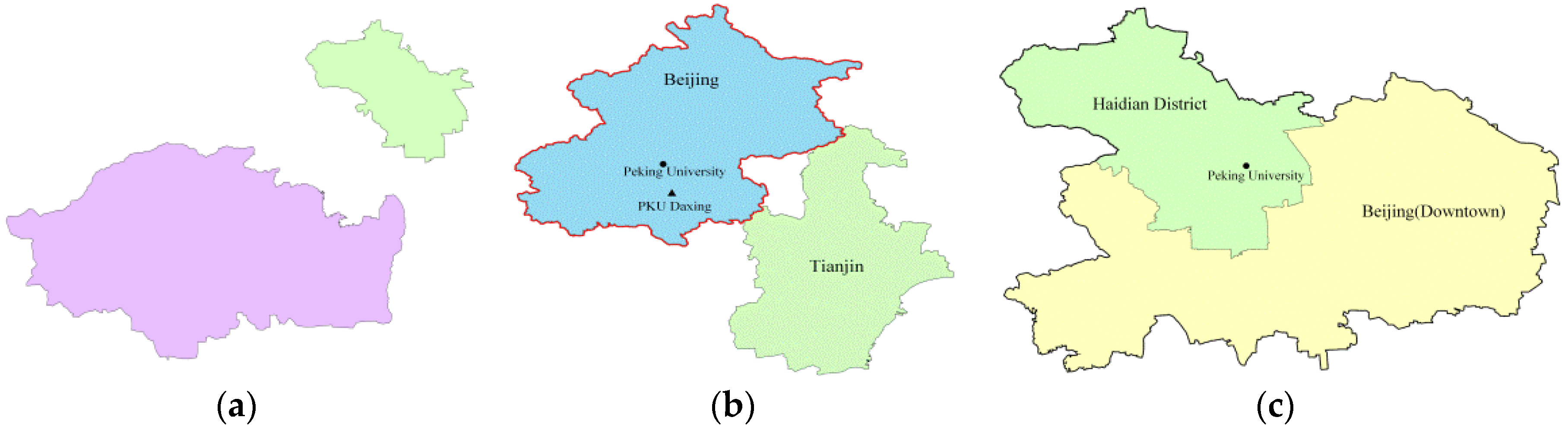
Scenario 2: The area suggested by point m contains the area of point i. For example, the query is “Beijing”, and there are documents referring to “Peking University”, “PKU DaXing”, and “Tianjin” (Figure 4b). For these three places, “Peking University” and “PKU Daxing” are included in Beijing. Tianjin and Beijing are neighbor cities and have no overlapping areas. We define both of the distances, the distance between Beijing and Peking University and the distance between Beijing and PKU Daxing, as $d_2$, because Peking University and PKU Daxing are at the same level (without containing) and both are inside Beijing. Their proximity to Beijing cannot be further differentiated. The relationship between Beijing and Tianjin fits the scenario 1, so the distance will be larger than $d_2$, which will finally lead to a lower score in comparison with Peking University/PKU Daxing. To summarize, for every location within the query area, we allocate the same distance ($d_2$) to get the same ranking score.

(c)

Scenario 3: The geographic scope of point m is contained by the scope of point i. For example, the query is “Peking University” and two documents refer to Beijing and Haidian District, respectively (Figure 4c). We decide that although the two areas both contain the query area, Haidian District is more relevant because its granularity is finer. To realize this, distances are defined as $d_3$. Because the fine-grained area’s radius is shorter than a coarse-grained one, the fine-grained area’s ranking will be higher.

In the process of proximity evaluation, the real case is always a mixture of the above three situations (Figure 5). The circle Q represents the query area, and circles P₁ to P₆ represent the areas of each point in the footprint. Circles P₁ and P₂ are contained by Q, which fit the scenario 2, i.e., the area mentioned in the document is contained by the query area. Thus, the distance is defined as R_q for both P₁ and P₂, because there is no other information to differentiate the relevance of these two places. Circles P₃ and P₄ fit the scenario 3 because circles P₃ and P₄ both contain Q, and the distances are defined as the radius of the places that contain the query area, which R₃ and R₄ respectively. Circles P₅ and P₆ fit scenario (1). Because circles P₅ and P₆ are separated from the query area, the distances are defined as the centroid distances, which are D₅ and D₆. According to the illustration, the retrieval ranking results for query area Q will be Rank(P₁) = Rank(P₂) > Rank(P₃) > Rank(P₄) > Rank(P₅) > Rank(P₆), because R_q < R₃ < R₄ < D₅ < D₆. This result conforms to common sense.

However, in the above steps, we decide which distance ($d_1,d_2,d_3$) will be chosen based on the awareness of topological relationships. How can we choose the distance if we do not know the topology beforehand?

• In scenario (2), for instance, P₁ and Q, d₃ < d₁ < d₂ and the final determined distance is d₂ (or R_q).
• In scenario (3), for instance, P₃ and Q, d₂ < d₁ < d₃ and the final determined distance is d₃ (or R₃).
• In scenario (1), for instance, P₅ and Q, d₃ < d₂ < d₁ and the final determined distance is d₁.

To summarize, the final distance d_i|m that we use in the similarity evaluation in all of the scenarios can be generalized as Equation (9). Therefore, in the retrieval process, we no longer have to examine the topological relationships. Instead, we only need to calculate d₁, d₂, and d₃ and set the final distance as the maximum among them, which will reduce the workload dramatically.

d_i|m = max(d₁, d₂, d₃)

(9)

Because there is often more than one point in the footprint of a document or queries, the effects of all of the points are summed. The general function is denoted as Equation (10), where the meanings of the symbols are identical with the former ones. This method can address the multi-scale problem and avoid the mistakes caused by the defects of the simple point-set model. Because this evaluation method describes the real searching scenario more precisely, the corresponding ranking results will be more accurate.

$$G_{I|Q}={\displaystyle \sum }_{m=1}^M{\displaystyle \sum }_{i=1}^{N_I}\frac{1}{d_{i|m}^r}$$

(10)

3.2. Frequency Weight Parameter

We represent the gravity model function above to evaluate the spatial proximity based on distance. However, proximity and similarity are not exactly equivalent. Similarity assesses not only the proximity but also the emphasis of the documents. We know that higher frequency of a word appearing in the document suggests higher probability of relevance. This characteristic is widely and successfully used in IR for stop-words filtering in various subject fields including text summarization and classification, such as the TF-IDF weight factor [13]. Unlike MBRs, which treats every point within the rectangle equally, the consideration of frequency in this article reflects the density of the points and the result can be more precise and sound. For instance, suppose that we have two documents with the same word capacities and footprints. The word capacity is 1000 for each document, and both documents refer to Beijing. Document A recommends Beijing 100 times, whereas B only recommends Beijing 10 times. The conclusion drawn from MBR analysis could be that A and B have the same score for the query of “Beijing” because their MBRs are identical. However, in the common sense of relevance, document A is probably more relevant to Beijing than document B. By introducing the frequency factor, such deficiencies may be avoided.

The frequency of the spatial location i is defined as f_i in Equation (11), where n_i is the occurrence number of place names referring to any location i and N_I is the total occurrence of place names in the corresponding document. It should be noted that the frequency is calculated based on geographic semantics rather than spelling, so the occurrence counts aliases referring to an identical geographic location can be accumulated, even though the expressions may be completely different. Higher f_i suggests higher relevance of the document to the spatial location.

$$f_i=\frac{n_i}{{{\displaystyle \sum }}_{j=1}^{N_I}{n}_j}$$

(11)

To combine the effects of both frequency and distance, we allocate the weight of distances between query points and document footprint points in direct proportion to the frequency of corresponding place name occurrences in a single document. Therefore, the gravity model in Equation (3) can be adjusted to Equation (12). The parameter r in the equation is an empirical value to coordinate the influence of frequency and spatial distance. With the increase in r, spatial distance becomes more decisive.

$$g_{i|m}=f_i\times \frac{1}{d_{i|m}^r}$$

(12)

The normalized evaluation function of the whole document will be calculated as equation (13). Considering that the spatial location m in a query may appear more than once, the parameter f_m is its frequency in the query. Equation (14) is a simplified version that ignores the frequency of points in the query. |D| is the number of documents in the corpus, and the rest of the denotations are identical with the former equations.

$$G_{I|Q}=\frac{{{\displaystyle \sum }}_{m=1}^M{f}_m{{\displaystyle \sum }}_{i=1}^{N_i}{f}_i\frac{1}{d_{i|m}^r}}{{{\displaystyle \sum }}_{I=1}^{\left|D\right|}{{\displaystyle \sum }}_{m=1}^M{f}_m{{\displaystyle \sum }}_{i=1}^{N_I}{f}_i\frac{1}{d_{i|m}^r}}$$

(13)

$$G_{I|Q}=\frac{{{\displaystyle \sum }}_{m=1}^M{{\displaystyle \sum }}_{i=1}^{N_i}{f}_i\frac{1}{d_{i|m}^r}}{{{\displaystyle \sum }}_{I=1}^{\left|D\right|}{{\displaystyle \sum }}_{m=1}^M{{\displaystyle \sum }}_{i=1}^{N_I}{f}_i\frac{1}{d_{i|m}^r}}$$

(14)

The algorithm synthesizes the effect of both frequency and distance. By ranking G_I|Q scores in descending orders, we obtain a list whose top items are the most relative results for the query.

3.3. Ranking Method

3.3.1. Pre-Filtering and Spatial Index

There is one defect of the frequency-distance-based evaluation algorithm. If a document contains locations that are very close to the query point, but the frequencies of these locations are low, the combined score for the document may not rank high enough to allow the document be retrieved. To conquer this irrationality, we set a rule that if the document contains locations that are close enough to the query point, the document must be returned as a result and then be ranked. We realize this principle by adding a filter step in runtime.

Before computing the similarity scores, for each document, we calculate the minimum distance between the query point m and points in the document’s footprint, then retrieve the documents with the top W-shortest minimum distances to generate a candidate set for the query. The similarity evaluation will only be performed on the candidate. This step will ensure that the principle mentioned above is applied and it will also lessen workloads. In practice, the value of W is decided considering the total documents in the corpus.

A spatial index based on geohash is built to accelerate the filtering. Invented by Niemeyer [33], geohash is a latitude/longitude geocode system and is suitable for spatial point indexing. Geohash subdivides space into grid-shaped buckets called geohashes, and every bucket has a unique string code. Because our footprint model is point-based and takes areas into consideration synchronically, geohash is suitable and applied in our work. We use seven digits to code the points in the documents’ footprints, reaching a precision of ±0.076 km. The index records the code string and IDs of documents whose footprint contain this code.

It is a great advantage that the geohash index converts spatial information into strings. Therefore, the neighborhood searching by comparing geohash codes is performed through spatial filtering instead of distance calculation. In addition, by employing the idea of seed filling algorithm, we can quickly obtain the top W documents containing nearest locations to the query point.

The pre-filtering procedure is illustrated as Figure 6. Once the spatial query is submitted, its footprints are encoded in geohash and pushed into a target list. Select the documents whose footprint contains the target geohash string as the candidates. If the number of candidates is less than the threshold that we set, more candidates should be selected. To obtain more candidates, we push the geohash codes of the target grid’s eight neighbors into the target list. Repeat the steps above, and the pre-filtering procedure ends when the number of candidates achieves the threshold.

3.3.2. Ranking Procedure

The overall spatial ranking procedure is illustrated in Figure 7. After a query is submitted, we perform a geohash pre-filtering to generate a candidate list; compute the ranking score for each document in the list by applying the evaluation algorithm proposed in Section 3; and sort documents according to the ranking scores in descending order and return the result. It should be noticed that, after calculating the frequencies of points in a candidate document, we can sort the points in descending order of f_i and extract the top K points to represent the document’s footprint. This step will decrease the number of points to be involved in distance calculation and reduce the calculation amount dramatically.

The time complexity of our algorithm is O(M × K × W). Among the three factors influencing the efficiency, the number of spatial locations mentioned by a query (M) is small, usually less than 5, and parameter K is an empirical constant. Hence, parameter W is the decisive factor of efficiency. The value of W is proportional to the total document number of the corpus. Thus, the time complexity can be simplified as O(n).

4. Experiments and Results

4.1. Data Source

The corpus we used in our experiment consists of the domestic news of China crawled from Sina News [34] from June to December 2014. There are 700 documents in the corpus, and each document contains 1 to 29 place names. The scales of the spatial locations referred to vary from one single POI to a province.

Two footprint models are built in preprocessing based on this corpus. One is the traditional document’s overall MBR model, computed by the coordinates of contained place names that derive from the gazetteer, used as a reference. The other footprint model is the point-set-based model that we proposed. To test the robustness of our model in dealing with various scenarios, 50 queries of different scales are specifically chosen, which consider all of the possible situations. Some of the queries are listed in

Table 1. Examples of queries.

Hierarchy Level	Instance
POI	Tsinghua University, PSB of Wenzhou …
District	Chaoyang district of Beijing, Wen’an county of Langfang …
City	Qingdao, Hankou …
Province	Ningxia Autonomous Region, Hong Kong …

.

4.2. Criteria

We choose precision, recall, average precision (AP), mean average precision (MAP), and R-precision, which are defined as Equations (15)–(19), to assess the performance of our model. Experiments based on the MBR binary model and MBR area ratio model serve as a comparison.

$$Precision=\frac{R_a}{A}$$

(15)

$$Recall=\frac{R_a}{R}$$

(16)

$$AP=\left({\displaystyle \sum }_{i=1}^R\frac{i}{ran{k}_i}\right)/R$$

(17)

$$MAP=\left({\displaystyle \sum }_{i=1}^{Q}A{P}_i\right)/Q$$

(18)

$$R-Precision=\left({\displaystyle \sum }_{i=1}^Q{P}_i@R\right)/Q$$

(19)

In Equation (15) to Equation (19), R_a represents the documents that are retrieved and relevant; A represents the documents that are retrieved; R represents the documents that are relevant; rank_i represents the rank of relevant document i in the result list; Q represents the number of queries in a batch; and P_i@R represents the precision when the number of retrieved documents is R. The criteria with higher values indicate better performance of retrievals.

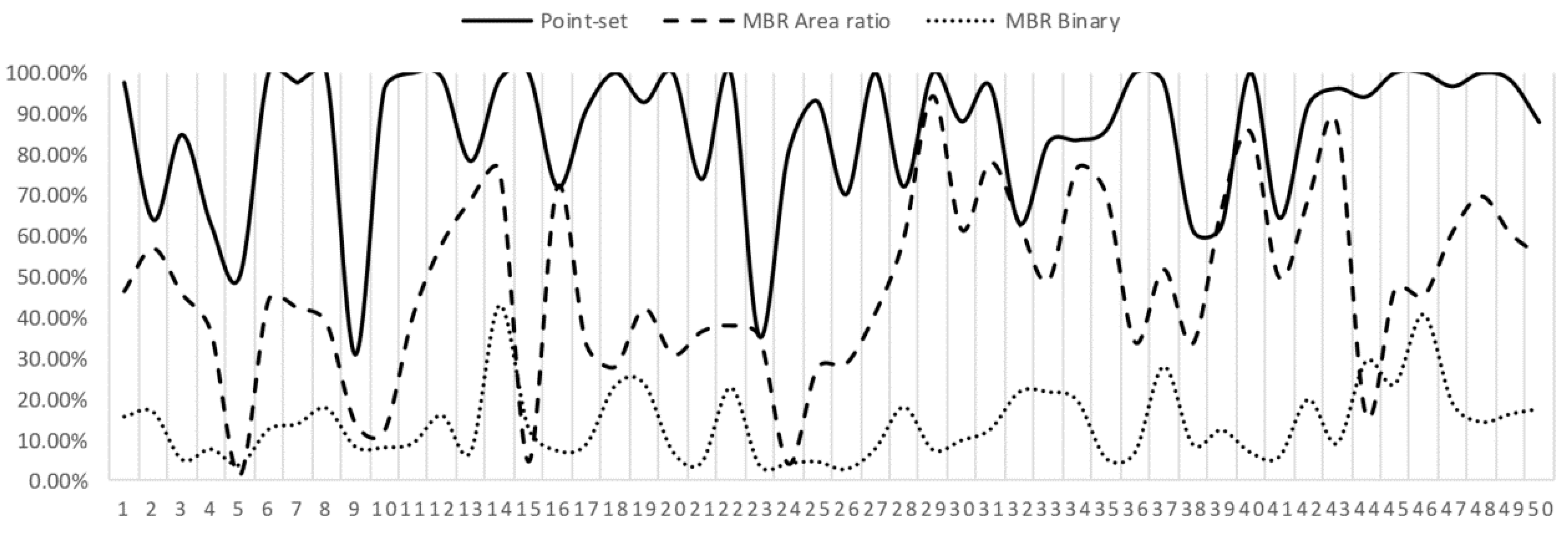
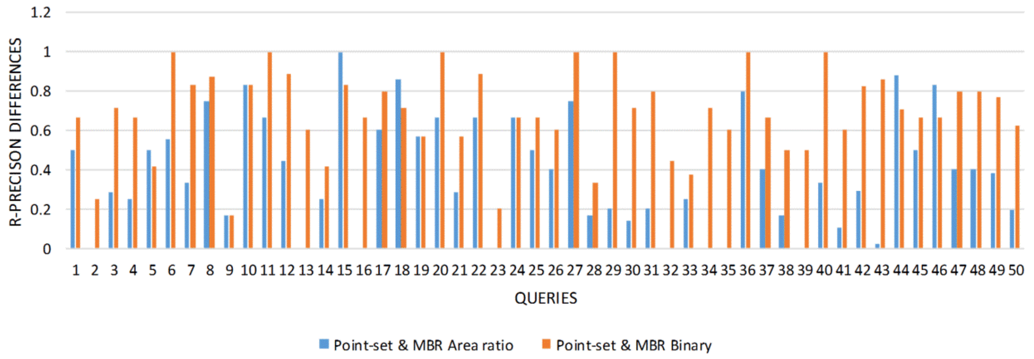
4.3. Performance Comparison

By applying the process shown in Figure 7, we obtained the retrieval results, from which the Precision-Recall (P-R) Curve (Figure 8), APs (Figure 9), MAPs (

Table 2. The MAPs of the three footprint models.

Models	MAP
Point-set	0.8479
MBR Area-ratio	0.4776
MBR Binary	0.1392

), and Query Histograms (Figure 10) are derived.

The P-R Curve of the point-set model is the highest, which indicates that our footprint model and evaluation algorithm achieve higher precisions than the MBR models under the same recall rates. In addition, the precision descending rate of the point-set model is low, which implies that the average precision of massive returns is acceptable.

For Figure 9, the performance of our algorithm is much better for most of the queries, such as queries 6–9 or 24–28, which focus on a relatively fine-grained area, such as Licheng district of Quanzhou city, Fujian province (query 6), and Nanchang University (query 27) and are more likely to be mentioned together with higher administrative units, such as cities and provinces. In that case, for these queries, the target locations will be swamped in the traditional MBR model. In addition, queries such as queries 9 (Guangdong province), 16 (Maoming city of Guangzhou province), 23 (Ningxia Autonomous Region), and 29 (Luoyang city) are coarse-grained locations and will survive from location swamping in the traditional MBR model.

The average precisions of our algorithm for 92.0% of queries are apparently higher than the other two models, and our algorithm’s MAP reaches 84.79%.

Query Histograms are generated as the differential of the R-Precision between different methods. The higher the column is, the better performance our algorithm obtains in comparison with MBR models. For 84% of queries, our method’s R-Precision is much higher.

In conclusion, all of these figures back up the assertion that the model and ranking algorithm that we proposed in this paper outperforms the MBR models, especially in dealing with documents whose footprints consist of fine-grained locations or locations of different hierarchy levels. This feature is very suitable for web-based geographic information retrieval, considering the multisource, unstructured characters of online information. In addition, POI is a very popular format of geographic information in online sources and is point set in nature.

5. Conclusions

In this paper, we propose a new point-set-based method to construct footprints for documents and a spatial ranking method based on that structure. The point-set-based model proposed is redundancy-free and conquers location swamping. Due to the dispersion property of spatial points, the frequency of a place name in a document can be taken into consideration as a weight factor, making the evaluation anisotropic and thus more precise. One of the key values of the model is that the model can address mixed-scale data without examining the topological relationship, which is rarely studied in related works, neither by the overall MBR model nor the MBR set model. In addition, a complete implementation procedure is provided, as well as optimizing plans based on geohash indexing. Experiments are carried out, and the results show that (1) our algorithm achieves higher precisions than the MBR models under the same recall rates, and its precision descending rate is much lower, assuring that the precision of massive returns will be guaranteed; (2) the accuracy of our algorithm is much higher than MBR methods when dealing with fine-grained queries, which means that our algorithm will be more suitable to obtain detailed information; and (3) the MAP of our algorithm reaches 84.79%, whereas the MAPs for the MBR models are 47.8% and 13.9%, respectively. All of these figures suggest that our algorithm outperforms the traditional methods in most cases.

References

1. Stats & Facts. Google Places. Available online: https://sites.google.com/a/pressatgoogle.com/googleplaces/metrics (accessed on 7 July 2014).
2. Neustar Localeze. Local Search Usage Study. Available online: http://www.localsearchstudy.com/ (accessed on 7 July 2014).
3. Larson, R.R. Geographic information retrieval and spatial browsing. In GIS and Libraries: Patrons, Maps and Spatial Information; Smith, L., Gluck, M., Eds.; Urbana-Champaign, University of Illinois: Champaign, IL, USA, 1995; pp. 81–124. [Google Scholar]
4. Jones, C.B.; Alani, H.; Tudhope, D. Geographical information retrieval with ontologies of place. In Proceedings of the Conference on Spatial Information Theory, Morro Bay, CA, USA, 19–23 September 2001; pp. 322–335.
5. Peters, C.; Clough, P.; Gey, F.C. Evaluation of Multilingual and Multi-modal Information Retrieval; Springer Science & Business Media: Medford, MA, USA, 2007. [Google Scholar]
6. Gey, F.; Larson, R.; Sanderson, M.; Joho, H.; Clough, P.; Petras, V. GeoCLEF: The CLEF 2005 cross-language geographic information retrieval track overview. In Accessing Multilingual Information Repositories; Perters, C., Gey, F., Gonzalo, J., Müller, H., Jones, G.J.F., Kluck, M., Magnini, B., de Rijke, M., Eds.; Springer: Berlin, Germany, 2006; pp. 908–919. [Google Scholar]
7. Guillén, R. CSUSM experiments in GeoCLEF2005: Monolingual and bilingual tasks. In Accessing Multilingual Information Repositories; Perters, C., Gey, F., Gonzalo, J., Müller, H., Jones, G.J.F., Kluck, M., Magnini, B., de Rijke, M., Eds.; Springer: Berlin, Germany, 2006; pp. 956–962. [Google Scholar]
8. Kornai, A. Evaluating Geographic Information Retrieval; Springer: Berlin, Germany, 2006. [Google Scholar]
9. Larson, R.R.; Frontiera, P. Spatial ranking methods for geographic information retrieval (GIR) in digital libraries. In Lecture Notes in Computer Science 3232; Heery, R., Lyon, L., Eds.; Springer: Berlin, Germany, 2004; pp. 45–57. [Google Scholar]
10. Peter, C.; Deselaers, T.; Ferro, N.; Gonzalo, J.; Jones, G.J.F.; Kurimo, M.; Mandl, T.; Peas, A.; Petras, V. Evaluating Systems for Multilingual and Multimodal Information Access; Springer: Berlin, Germany, 2009. [Google Scholar]
11. Martins, B.; Calado, P. Learning to rank for geographic information retrieval. In Proceedings of the 6th Workshop on Geographic Information Retrieval, Zurich, Switzerland, 28–29 January 2010; ACM: New York, NY, USA, 2010. [Google Scholar]
12. Papadias, D.; Theodoridis, Y.; Sellis, T.; Egenhofer, M.J. Topological relations in the world of minimum bounding rectangles: A study with R-trees. Acm Sigmod Rec. 2010, 24, 92–103. [Google Scholar] [CrossRef]
13. Salton, G.; Buckley, C. Term-weighting approaches in automatic text retrieval. Inf. Process. & Manag. 1988, 24, 513–523. [Google Scholar]
14. Jones, C.B.; Abdelmoty, A.I.; Finch, D.; Fu, G.; Vaid, S. The SPIRIT spatial search engine: Architecture, ontologies and spatial indexing. Lect. Notes Comput. Sci. 2004, 3234, 125–139. [Google Scholar]
15. Purves, R.S.; Clough, P.; Jones, C.B.; Arampatzis, A.; Bucher, B.; Finch, D.; Fu, G.; Joho, H.; Syed, A.K.; Vaid, S.; et al. The design and implementation of SPIRIT: A spatially aware search engine for information retrieval on the Internet. Int. J. Geogr. Inf. Sci. 2007, 21, 717–745. [Google Scholar] [CrossRef]
16. Zhou, Y.; Xie, X.; Wang, C.; Gong, Y.; Ma, W. Hybrid index structures for location-based web search. In Proceedings of the 14th ACM International Conference on Information and Knowledge Management, Bremen, Germany, 31 October–5 November 2005; pp. 155–162.
17. Chen, Y.; Suel, T.; Markowetz, A. Efficient query processing in geographic web search engines. In Proceedings of the ACM SIGMOD International Conference on Management of Data, Chicago, IL, USA, 27–29 June 2006; pp. 277–288.
18. De Andrade, F.G.; Baptista, C.S.; Davis, C.A. Improving geographic information retrieval in spatial data infrastructures. Geoinformatica 2014, 18, 793–818. [Google Scholar] [CrossRef]
19. De Sabbata, S.; Reichenbacher, T. Criteria of geographic relevance: An experimental study. Int. J. Geogr. Inf. Sci. 2013, 26, 1495–1520. [Google Scholar] [CrossRef]
20. Reichenbacher, T.; De Sabbata, S.; Purves, R.S.; Fabrikant, S.I. Assessing geographic relevance for mobile search: A computational model and its validation via crowdsourcing. J. Assoc. Inf. Sci. Technol. 2016. [Google Scholar] [CrossRef]
21. Ding, J.; Gravano, L.; Shivakumar, N. Computing geographical scopes of web resource. In Proceedings of the 26th International Conference on Very Large Data Bases, Cairo, Egypt, 10–14 September 2000.
22. Amitay, E.; Har’El, N.; Sivan, R.; Soffer, A. Web-a-where: Geotagging web content. In Proceedings of the 27th Annual International ACM SIGIR Conference on Research and Development in Information Retrieval, Sheffield, UK, 25–29 July 2004.
23. Adams, B.; Janowicz, K. Thematic signatures for cleansing and enriching place-related linked data. Int. J. Geogr. Inf. Sci. 2015, 29, 556–579. [Google Scholar] [CrossRef]
24. Ferrés, D.; Rodríguez, H. Evaluating geographical knowledge re-ranking, linguistic processing and query expansion techniques for geographical information retrieval. In String Processing and Information Retrieval, Proceedings of the 22nd International Symposium, London, UK, 1–4 September 2015; Iliopoulos, C., Puglisi, S., Yilmaz, E., Eds.; pp. 311–323.
25. Nguyen, T.T.; Jung, J.J. Exploiting geotagged resources to spatial ranking by extending HITS algorithm. Comput. Sci. Inf. Syst. 2014, 12, 185–201. [Google Scholar]
26. Adams, B. Finding similar places using the observation-to-generalization place model. J. Geogr. Syst. 2015, 17, 137–156. [Google Scholar] [CrossRef]
27. Jiang, D.; Vosecky, J.; Leung, K.W.; Yang, L.; Ng, W. SG-WSTD: A framework for scalable geographic web search topic discovery. Knowl.-Based Syst. 2015, 84, 18–33. [Google Scholar] [CrossRef]
28. Rivera, F.M.; Ruiz, M.T.; Guzmám, G.; Ibarra, M.M. A collaborative learning approach for geographic information retrieval based on social networks. Comput. Hum. Behav. 2015, 51, 829–842. [Google Scholar] [CrossRef]
29. Mouratidis, K.; Li, J.; Tang, Y.; Mamoulis, N. Joint search by social and spatial proximity. IEEE Trans. Knowl. Data Eng. 2015, 27, 781–793. [Google Scholar] [CrossRef]
30. Liu, Y.; Yuan, Y.; Xiao, D.; Zhang, Y.; Hu, J. A point-set-based approximation for areal objects: A case study of representing localities. Comput. Environ. Urban Syst. 2010, 34, 28–39. [Google Scholar] [CrossRef]
31. Tobler, W.R. A computer movie simulating urban growth in the Detroit region. Econ. Geogr. 1970, 46, 234–240. [Google Scholar] [CrossRef]
32. Liu, Y.; Sui, Z.; Kang, C.; Gao, Y. Uncovering patterns of inter-urban trip and spatial interaction from social media check-in data. PLoS ONE 2014, 9, e86026. [Google Scholar] [CrossRef] [PubMed]
33. Neimeyer, G. Geohash Tips & Tricks. Available online: http://geohash.org/site/tips.html (accessed on 1 June 2016).
34. Sina News. Available online: http://roll.news.sina.com.cn/news/gnxw/gdxw1/index.shtml (accessed on 1 January 2015).
Figure 1. The space redundancies caused by the MBR model and convex hull model. The black dots denote the corresponding locations or areas referred to by place names in a document.
Ijgi 05 00122 g001
Figure 2. The sketch map of the spatial relations between Beijing (Downtown), Haidian District, Dongcheng District, Peking University, the National Museum, and the center of Beijing.
Ijgi 05 00122 g002
Figure 3. An example of a place name whose area information can be obtained from gazetteers.
Ijgi 05 00122 g003
Figure 4. Sketch maps of the three scenarios of regional relationships. (a) Scenario 1: the point m and the point i do not completely contain each other; (b) Scenario 2: the area suggested by point m contains the area of point I; (c) Scenario 3: the geographic scope of point m is contained by the scope of point i.
Ijgi 05 00122 g004
Figure 5. The relationship between the areas of the query and the document according to the three scenarios.
Ijgi 05 00122 g005
Figure 6. The procedure of geohash pre-filtering.
Ijgi 05 00122 g006
Figure 7. The overall spatial ranking process of the point-set based footprint model.
Ijgi 05 00122 g007
Figure 8. The Precision-Recall Curve of three footprint models.
Ijgi 05 00122 g008
Figure 9. The Aps of the three footprint models.
Ijgi 05 00122 g009
Figure 10. The Query Histograms of the three footprint models.
Ijgi 05 00122 g010