
A GIS- and Fuzzy Set-Based Online Land Price Evaluation Approach Supported by Intelligence-Aided Decision-Making


Abstract
:1. Introduction
2. Online Land Price Evaluation Approach
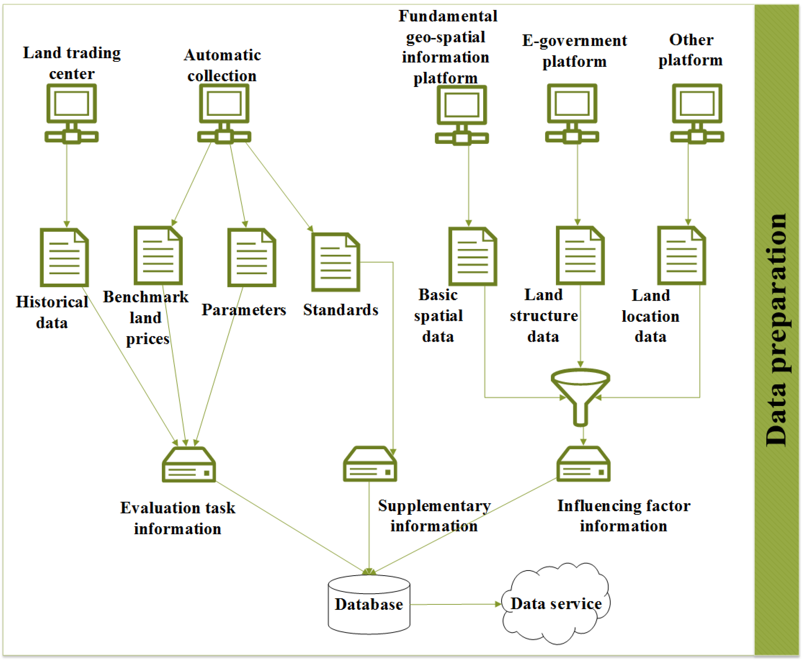
2.1. Data Sources
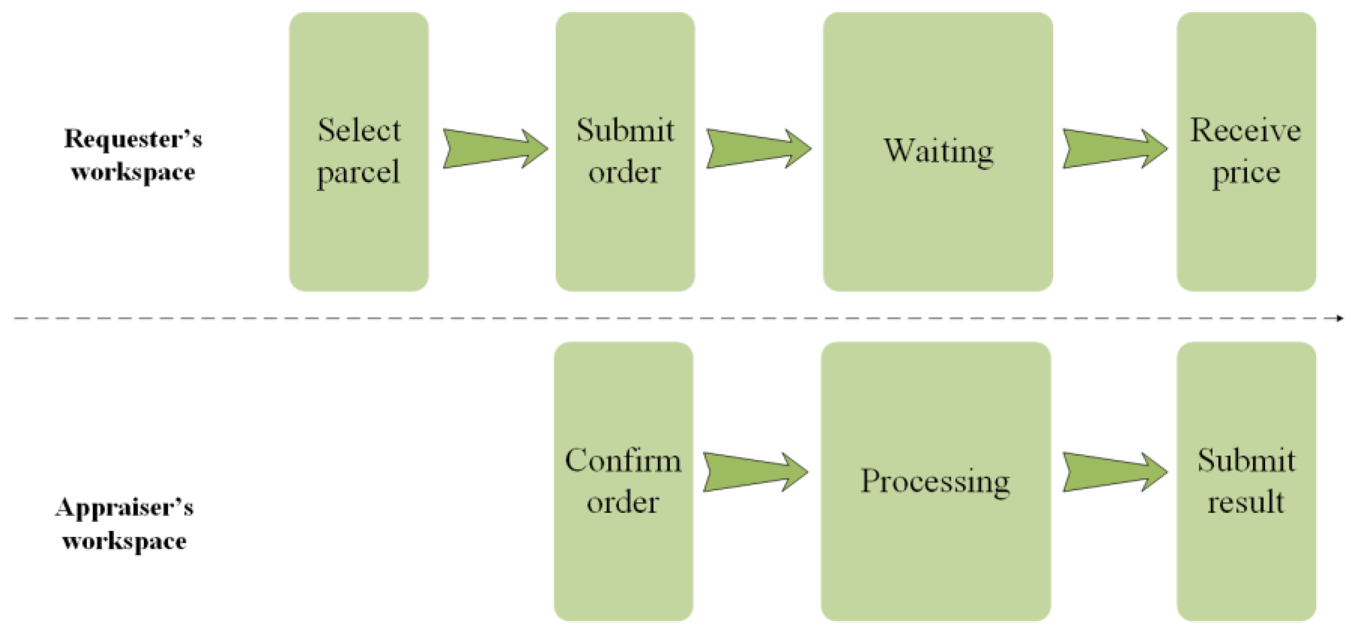
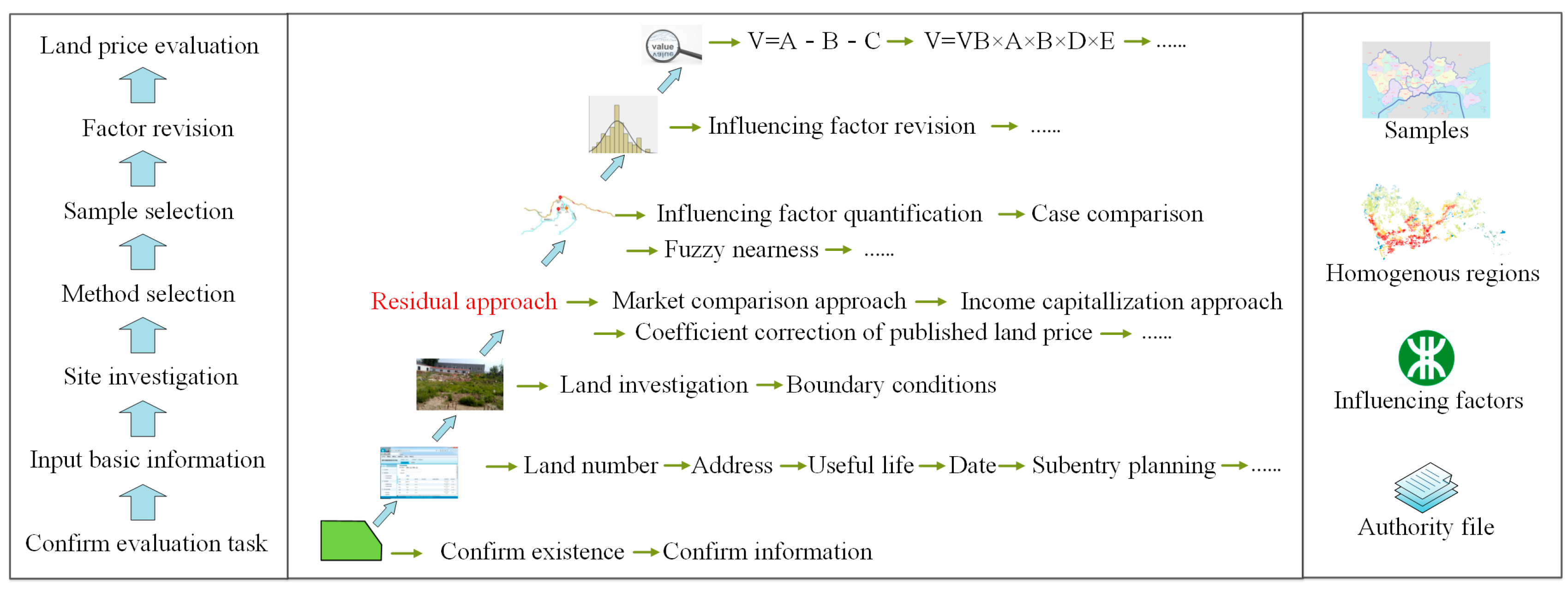
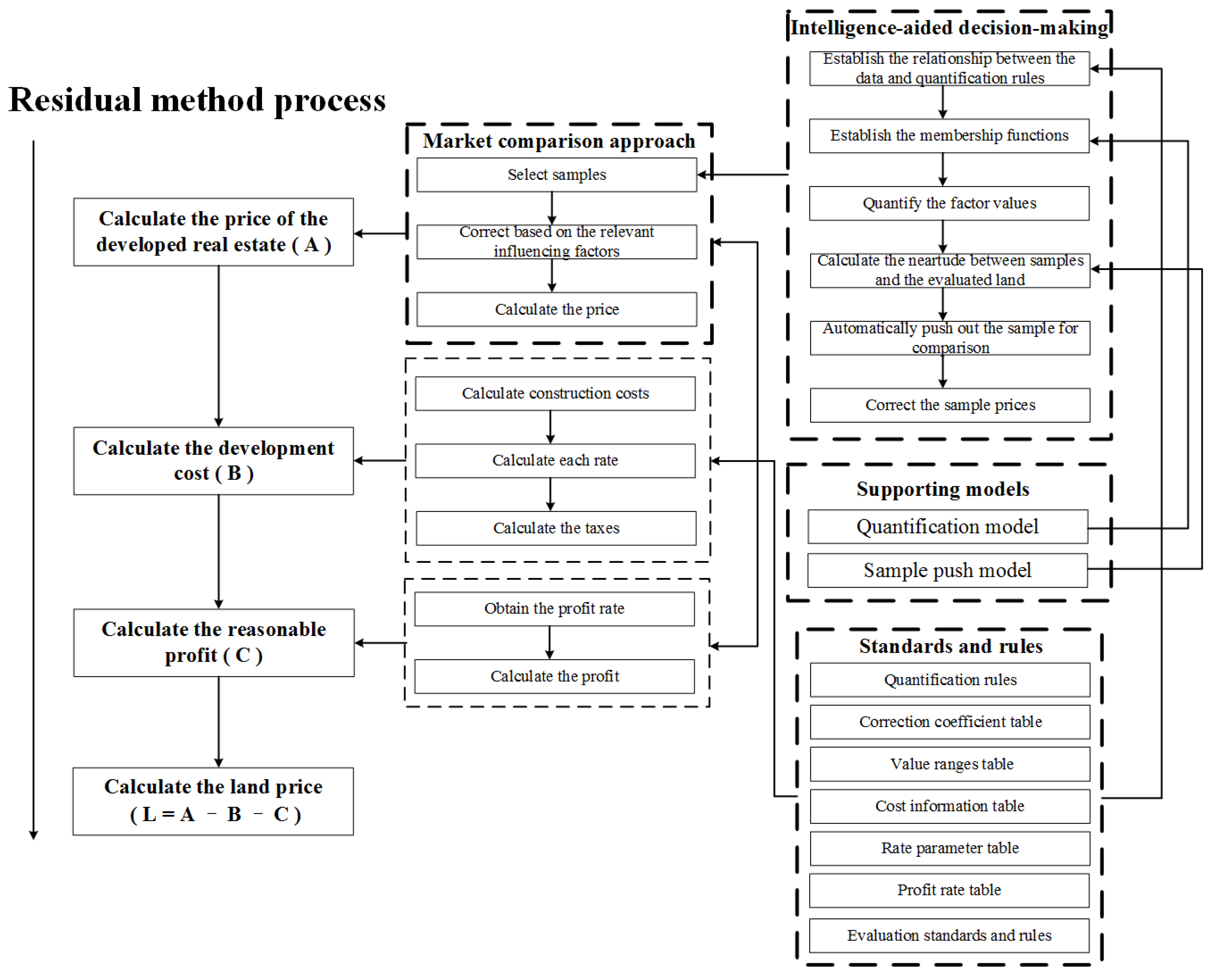
2.2. Task Flow
2.3. Intelligence-Aided Decision-Making Models
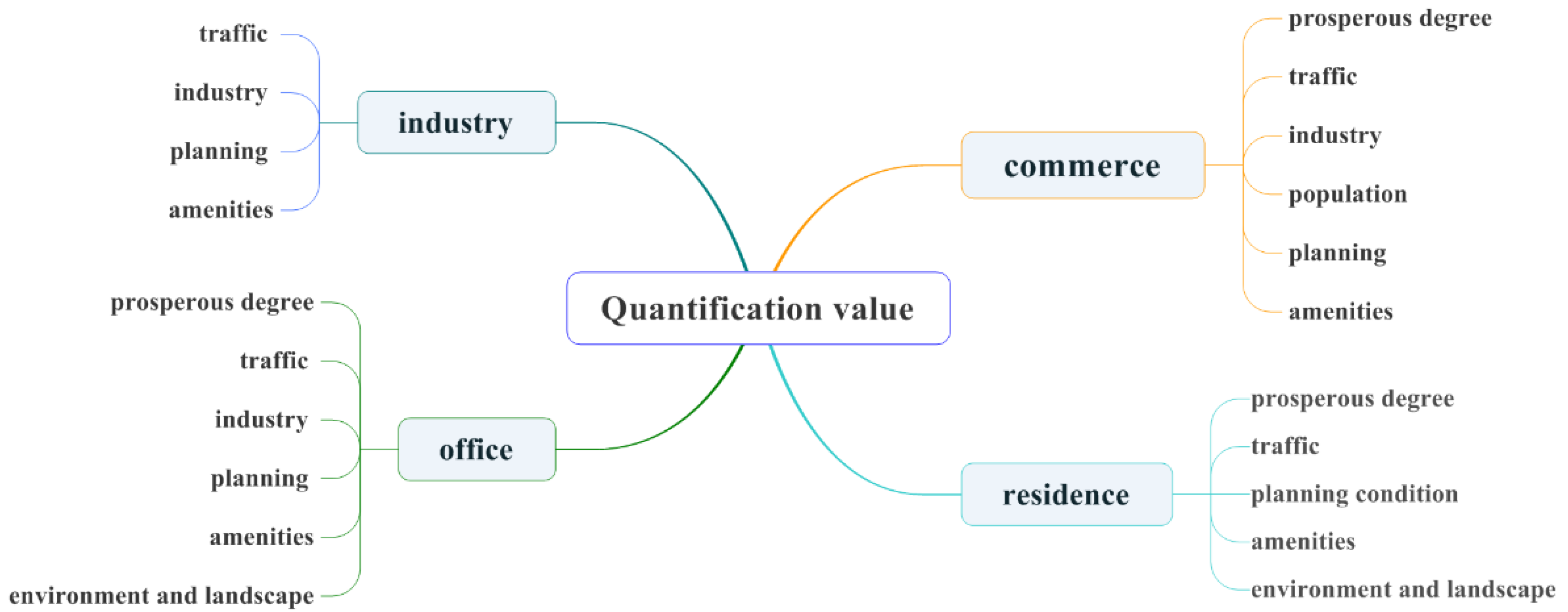
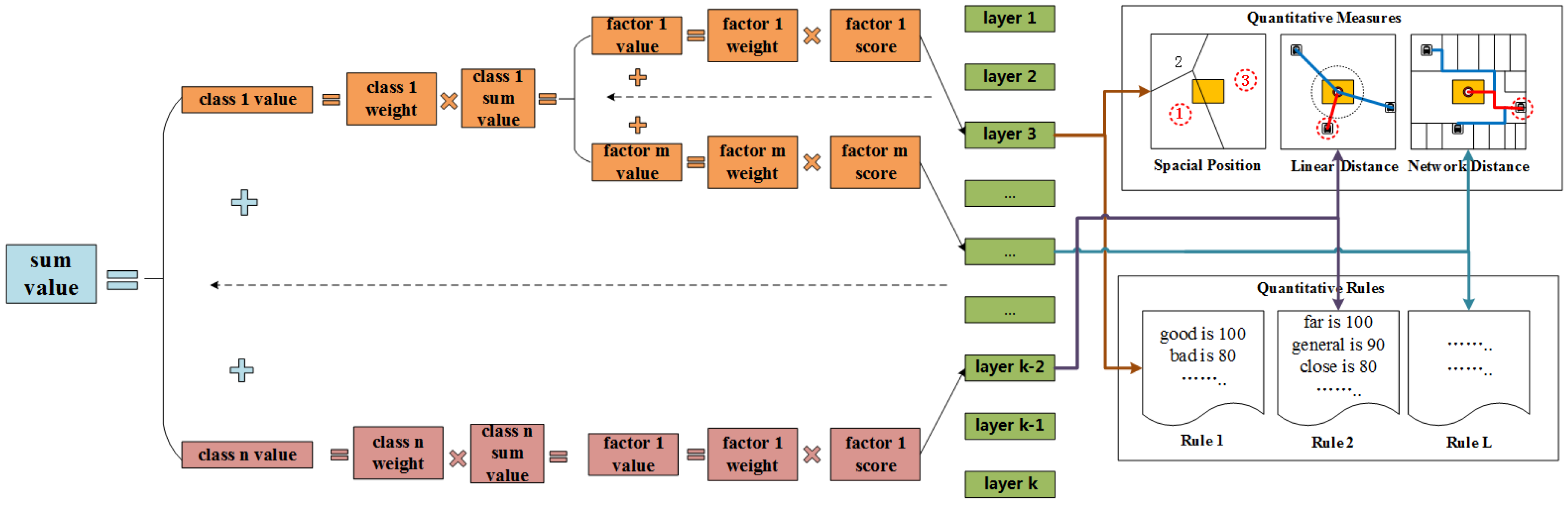
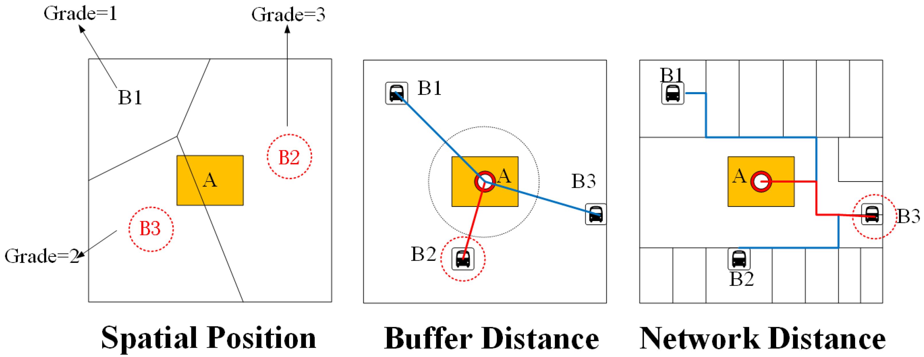
2.3.1. GIS- and Fuzzy Set-Based Location Factor Quantification Model
- If the shortest distance between factor B and land A is less than m, then the value is . If this distance lies in the range of m to m, then the value is or , where is a function that reflects the relationship between the quantitative value and the shortest distance. If this distance is greater than m, then the value is . For factors that are considered to be worse as their values increase, this model uses the trapezoidal distribution, as follows:
- On the condition that the location of land A is within the district of factor B, if the grade is , then the value is . If the grade is , then the value is If the grade is , then the value is If the location of land A is outside the district of factor B, then the value is . This model uses the following distribution function:
- 1.
- Related to spatial position:
- 2.
- Related to buffer distance:
- 3.
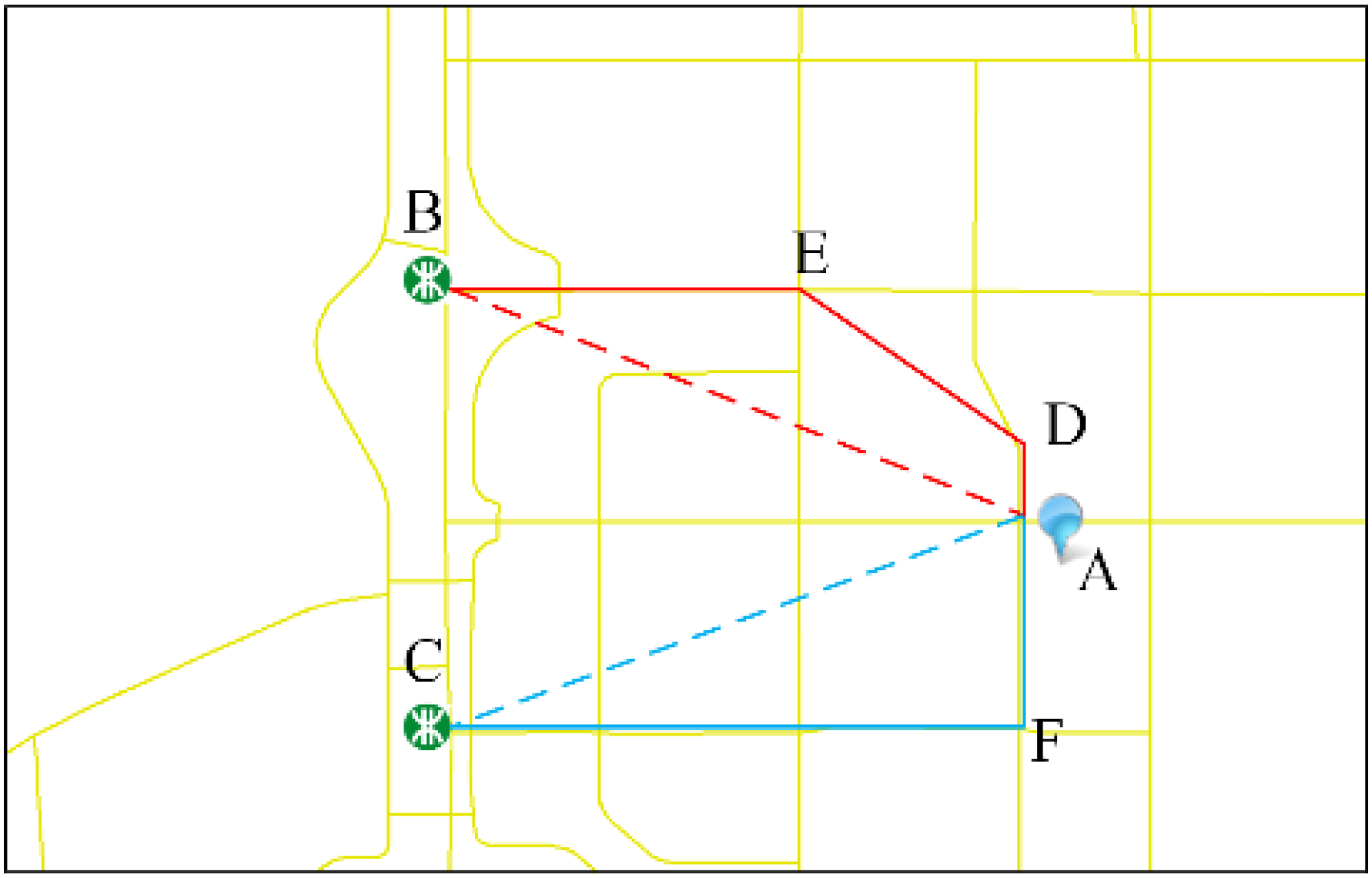
- Related to network distance:
2.3.2. Neartude-Based Transaction Sample Push Model
- (1)
- ;
- (2)
- (3)
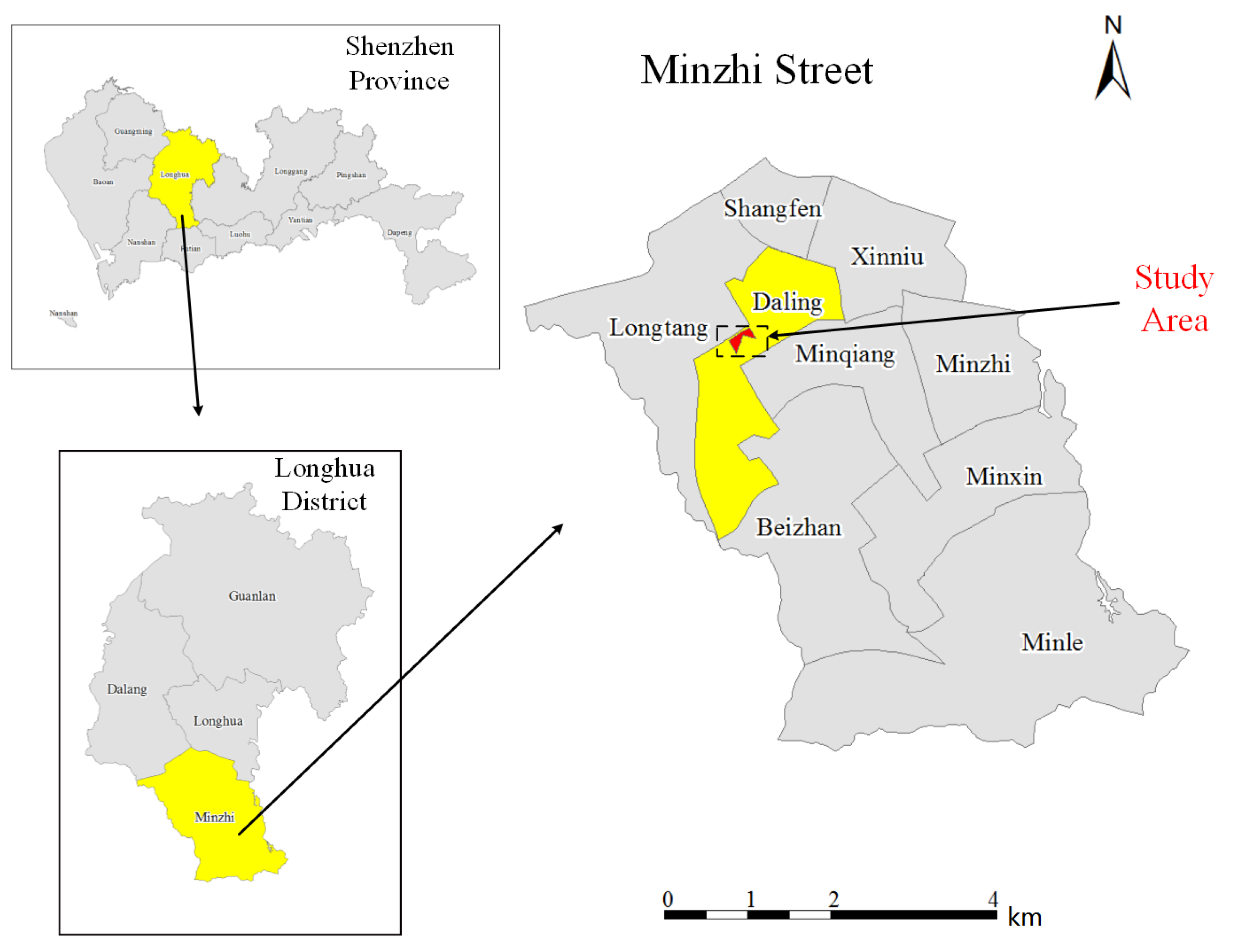
3. Study Area and Evaluation
3.1. Data Preparation
3.2. Implementation of the System Using the Residual Method
3.2.1. Calculate the Real Estate Price, Supported by Intelligence-Aided Decision-Making
- (1)
- Collected and analyzed related references from throughout the world.
- (2)
- Found case studies similar to Shenzhen.
- (3)
- Found experts who are specialized in research on the influence of location factors.
- (4)
- Designed a questionnaire similar to Table 1.
- (5)
- Posted the questionnaire online and sent the link of the website to the selected experts.
- (6)
- Requested the experts to fill in their own factors and weights.
- (7)
- Analyzed the received questionnaires and constructed a table similar to Table 1.
- (8)
- Sent the table to experts for review.
- (9)
- Iterated the above steps until all experts accepted the final table.
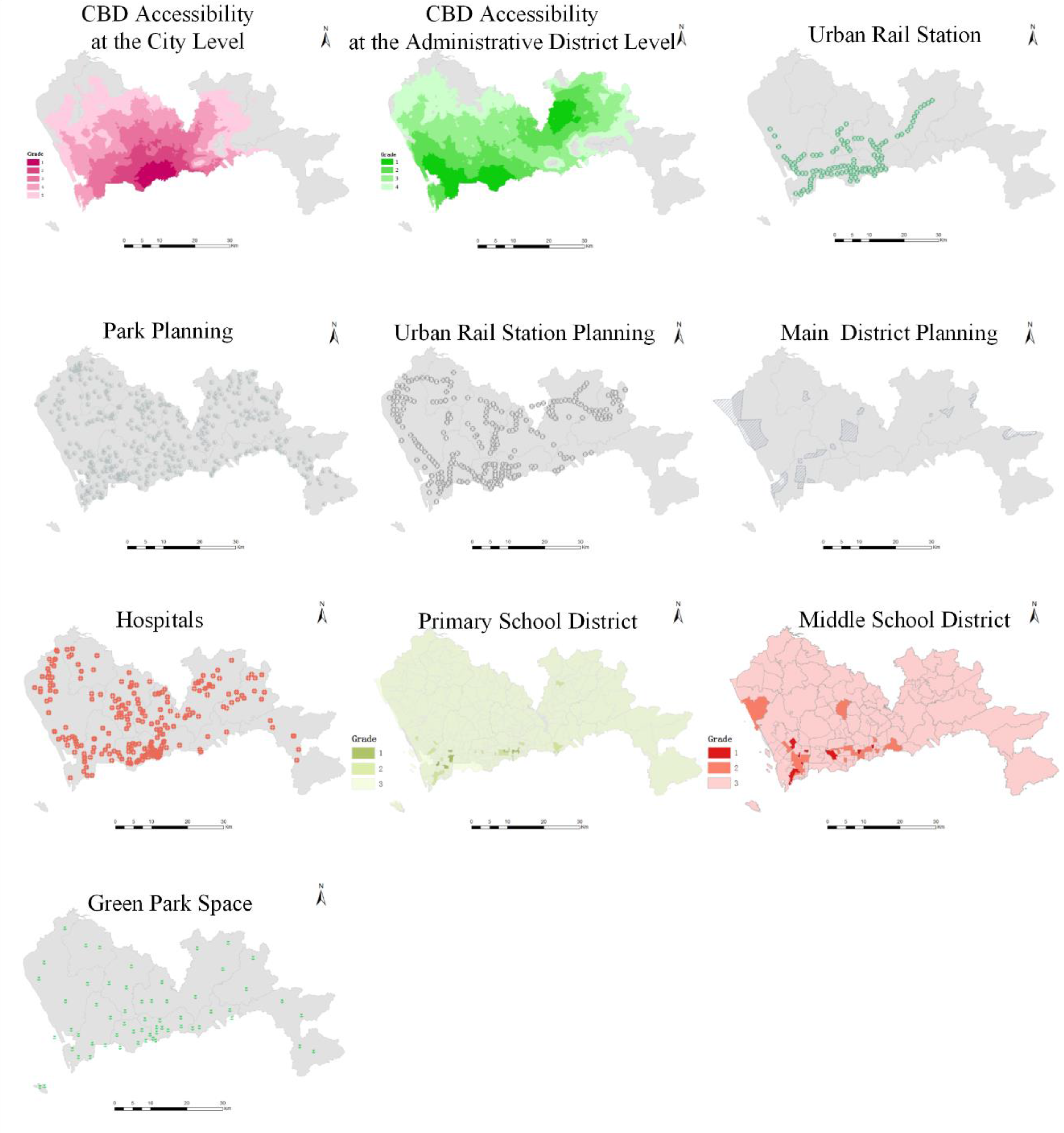
- Central business district (CBD) accessibility at the city level: This layer refers to the accessibility of the CBD based on the division of the area into several grades at the city level. Locations of Grade 1 are in the lowest-cost areas, and locations of Grade 5 are in the highest-cost areas.
- CBD accessibility at the administrative district level: This layer refers to the accessibility of the CBD based on the division of the area into several grades at the administrative district level. Locations of Grade 1 are in the lowest-cost areas, and locations of Grade 5 are in the highest-cost areas.
- Urban rail station: This layer refers to the network distance to the nearest urban rail station.
- Park planning: This layer refers to the network distance to the nearest planned location of a park.
- Urban rail station planning: This layer refers to the network distance to the nearest planned location of an urban rail station.
- Main district planning: This layer refers to the spatial relationship with respect to a planned main district.
- Hospitals: This layer refers to the network distance to the nearest hospital.
- Primary school district: In China, primary school districts are classified by the quality of education.
- Middle school district: In China, middle school districts are classified by the quality of education.
- Green park space: This layer refers to the network distance to a green space, such as a park.
3.2.2. Calculate the Land Price
4. Conclusions
Acknowledgments
Author Contributions
Conflicts of Interest
References
- Du, J.; Peiser, R.B. Land supply, pricing and local governments’ land hoarding in China. Reg. Sci. Urban Econ. 2014, 48, 180–189. [Google Scholar]
- Ding, G.; Gyourko, J.; Wu, J.; Ji, X. Land and house price measurement in China. National 2012, 99, 999–1006. [Google Scholar]
- Nasralla, Z.H. Design and implementation of Karbala real estate information system. In Proceedings of the First Scientific Conference, Johannesburg, South Africa, 2–3 December 2013.
- Vries, P.D.; Faber, R. Towards a real estate monitoring information system in Romania. Rom. J. Econ. Forecast. 2009, 12, 187–214. [Google Scholar]
- Saefuddin, A.; Widyanings, Y.; Ginting, A.; Mamat, M. Land price model considering spatial factors. Asian J. Math. Stat. 2012, 5, 132–141. [Google Scholar]
- Brasington, D.M.; Hite, D. Demand for environmental quality: A spatial hedonic analysis. Reg. Sci. Urban Econ. 2005, 35, 57–82. [Google Scholar] [CrossRef]
- Kong, F.; Yin, H.; Nakagoshi, N. Using GIS and landscape metrics in the hedonic price modeling of the amenity value of urban green space: A case study in Jinan city, China. Landsc. Urban Plan. 2007, 79, 240–252. [Google Scholar] [CrossRef]
- Kisilevich, S.; Keim, D.; Rokach, L. A GIS-based decision support system for hotel room rate estimation and temporal price prediction: The hotel brokers’ context. Decis. Support Syst. 2013, 54, 1119–1133. [Google Scholar] [CrossRef]
- Cheng, E.W.L.; Yu, L.; Li, H. A GIS-based site selection system for real estate projects. Constr. Innov. 2005, 5, 231–241. [Google Scholar]
- Yang, Y.; Sun, Y.; Li, S.; Zhang, S.; Wang, K.; Hou, H.; Xu, S. A GIS-based web approach for serving land price information. IJGI 2015, 4, 2078–2093. [Google Scholar] [CrossRef]
- Papadimitriou, F.; Mairota, P. Spatial scale-dependent policy planning for land management in southern Europe. Environ. Monit. Assess. 1996, 39, 47–57. [Google Scholar] [CrossRef] [PubMed]
- Papadimitriou, F. Artificial intelligence in modelling the complexity of Mediterranean landscape transformations. Comput. Electron. Agric. 2012, 81, 87–96. [Google Scholar] [CrossRef]
- Papadimitriou, F. Modelling landscape complexity for land use management in Rio de Janeiro, Brazil. Land Use Policy 2012, 29, 855–861. [Google Scholar] [CrossRef]
- Zeng, T.Q.; Zhou, Q. Optimal spatial decision making using GIS: A prototype of a real state geographical information system (Regis). Int. J. Geogr. Inform. Sci. 2001, 15, 307–321. [Google Scholar] [CrossRef]
- Wu, J.; Wang, M.; Li, W.; Peng, J.; Huang, L. Impact of urban green space on residential housing prices: Case study in Shenzhen. J. Urban Plan. Dev. 2015, 141, 05014023. [Google Scholar] [CrossRef]
- Sirmans, G.S.; Macpherson, D.A.; Zietz, E.N. The composition of hedonic pricing models. J. Real Estate Lit. 2005, 13, 3–43. [Google Scholar]
- Craven, B.D.; Islam, S.M. Ordinary Least-Squares Regression; Sage Publications: Thousand Oaks, CA, USA, 2011. [Google Scholar]
- Kwong, C.K.; Ip, W.H.; Chan, J.W.K. Combining scoring method and fuzzy expert systems approach to supplier assessment: A case study. Integr. Manuf. Syst. 2002, 13, 512–519. [Google Scholar] [CrossRef]
- Mayer, J.D.; Salovey, P.; Caruso, D.R.; Sitarenios, G. Measuring emotional intelligence with the MSCEIT V2.0. Emotion 2003, 3, 97–105. [Google Scholar] [CrossRef] [PubMed]
- Saaty, T.L. How to make a decision: The analytic hierarchy process. Eur. J. Oper. Res. 1990, 48, 9–26. [Google Scholar] [CrossRef]
- Dalkey, N.; Helmer, O. An experimental application of the Delphi method to the use of experts. Manag. Sci. 1963, 9, 458–467. [Google Scholar] [CrossRef]
- He, Y.; Liu, G. Research on comprehensive application of DEM and GIS spatial overlay analysis technology in land quantitative evaluation. Comput. Eng. 2006, 1, 088. [Google Scholar]
- Xiang, W. GIS-based riparian buffer analysis: Injecting geographic information into landscape planning. Landsc. Urban Plan. 1996, 34, 1–10. [Google Scholar] [CrossRef]
- Haggett, P.; Chorley, R.J. Network Analysis in Geography; Edward Arnold: London, UK, 1969. [Google Scholar]
- Zadeh, L.A. Fuzzy sets. Inf. Control 1965, 8, 338–353. [Google Scholar] [CrossRef]
- Bellman, R.E.; Zadeh, L.A. Decision-making in a fuzzy environment. Manag. Sci. 1970, 17, B141–B164. [Google Scholar] [CrossRef]
- Zavadskas, E.K.; Turskis, Z.; Ustinovichius, L.; Shevchenko, G. Attributes weights determining peculiarities in multiple attribute decision making methods. Eng. Econ. 2010, 21, 32–43. [Google Scholar]
- Fan, Z.; Ma, J.; Zhang, Q. An approach to multiple attribute decision making based on fuzzy preference information on alternatives. Fuzzy Sets Syst. 2002, 131, 101–106. [Google Scholar] [CrossRef]
- Ponsard, C. Fuzzy mathematical models in economics. Fuzzy Sets Syst. 1988, 28, 273–283. [Google Scholar] [CrossRef]
- Burrough, P.A. Fuzzy mathematical methods for soil survey and land evaluation. J. Soil Sci. 1989, 40, 477–492. [Google Scholar] [CrossRef]
- Salski, A.R.; Bartels, F. A fuzzy approach to land evaluation. IASME Transl. 2005, 5, 774–780. [Google Scholar]
- Zimmermann, H.J. Fuzzy set theory. Wiley Interdiscip. Rev. Comput. Stat. 2010, 2, 317–332. [Google Scholar] [CrossRef]
- Zhang, R.; Du, Q.; Geng, J.; Liu, B.; Huang, Y. An improved spatial error model for the mass appraisal of commercial real estate based on spatial analysis: Shenzhen as a case study. Habitat Int. 2015, 46, 196–205. [Google Scholar] [CrossRef]
- Wang, P. Fuzzy Set Theory and its applications; Shanghai Scientific and Technical Publishers: Shanghai, China, 1983. [Google Scholar]
- Deng, Y.; Gyourko, J.; Wu, J. Land and House Price Measurement in China; National Bureau of Economic Research, Inc.: Cambridge, MA, USA, 2012. [Google Scholar]
- Shi, P.; Yuan, Y.; Zheng, J.; Wang, J.; Ge, Y.; Qiu, G. The effect of land use/cover change on surface runoff in Shenzhen region, China. CATENA 2007, 69, 31–35. [Google Scholar] [CrossRef]
- Irwin, E.G.; Bockstael, N.E. The evolution of urban sprawl: Evidence of spatial heterogeneity and increasing land fragmentation. Proc. Natl. Acad. Sci. USA 2007, 104, 20672–20677. [Google Scholar] [CrossRef] [PubMed]


| Location Factor | Measure | Rule | Weight |
|---|---|---|---|
| CBD Accessibility at the City Level | Spatial Position | If the Grade of area the land located is 1, the score is 100; | 0.03 |
| If the Grade of area the land located is 2, the score is 95; | |||
| If the Grade of area the land located is 3, the score is 90; | |||
| If the Grade of area the land located is 4, the score is 85; | |||
| If the Grade of area the land located is 5, the score is 80; | |||
| Otherwise, the score is 80. | |||
| CBD Accessibility at the Administrative District Level | Spatial Position | If the Grade of area the land located is 1, the score is 100; | 0.06 |
| If the Grade of area the land located is 2, the score is 95; | |||
| If the Grade of area the land located is 3, the score is 90; | |||
| If the Grade of area the land located is 4, the score is 85; | |||
| If the Grade of area the land located is 5, the score is 80; | |||
| Otherwise, the score is 80. | |||
| Urban Rail Station | Network Distance | If the distance to the nearest station is 0 m to 500 m, the score is 100; | 0.15 |
| If the distance to the nearest station is 500 m to 1000 m, the score is 90; | |||
| If the distance to the nearest station is more than 1000 m, the score is 80. | |||
| Bus Stations | Network Distance | If the distance to the nearest station is 0 m to 300 m, the score is 100; | 0.06 |
| If the distance to the nearest station is 300 m to 500 m, the score is 90; | |||
| If the distance to the nearest station is more than 500 m, the score is 80. | |||
| Park Planning | Network Distance | If the distance to the nearest planned park is 0 m to 1000 m, the score is 100; | 0.02 |
| If the distance to the nearest planned park is over 1000 m, the score is 90. | |||
| Urban Rail Station Planning | Network Distance | If the distance to the nearest planned station is 0 m to 1000 m, the score is 100; | 0.02 |
| If the distance to the nearest planned station is more than 1000 m, the score is 90. | |||
| Main District Planning | Spatial Position | If the land is in the planned district, the score is 100; | 0.02 |
| If the land is outside of any planned district, the score is 90. | |||
| School Planning | Spatial Position | If the land is in a planned district, the score is 100; | 0.02 |
| If the land is outside of any planned district, the score is 90. | |||
| Disadvantageous Facility Planning | Buffer Distance | If the distance to the nearest facility is 0 m to 1000 m, the score is 80; | 0.02 |
| If the distance to the nearest facility is more than 1000 m, the score is 100. | |||
| Hospitals | Network Distance | If the distance to the nearest hospital is 0 m to 500 m, the score is 90; | 0.06 |
| If the distance to the nearest hospital is 500 m to 2000 m, the score is 100; | |||
| If the distance to the nearest hospital is more than 2000 m, the score is 80. | |||
| Kindergartens | Network Distance | If the distance to the nearest kindergarten is 0 m to 1000 m, the score is 100; | 0.06 |
| If the distance to the nearest kindergarten is more than 1000 m, the score is 90. | |||
| Primary School District | Spatial Position | If the Grade of district the land located is 1, the score is 100; | 0.06 |
| If the Grade of district the land located is 2, the score is 90; | |||
| If the Grade of district the land located is 3, the score is 80. | |||
| Middle School District | Spatial Position | If the Grade of district the land located is 1, the score is 100; | 0.12 |
| If the Grade of district the land located is 2, the score is 90; | |||
| If the Grade of district the land located is 3, the score is 80. | |||
| Green Park Space | Network Distance | If the distance to the nearest park is 0 m to 1000 m, the score is 100; | 0.2 |
| If the distance to the nearest park is 1000 m to 4000 m, the score is 90; | |||
| If the distance to the nearest park is more than 4000 m, the score is 80. | |||
| Seascape and Mountain Scenery | Buffer Distance | If the distance to the nearest scenic location is 0 m to 1000 m, the score is 100; | 0.1 |
| If the distance to the nearest scenic location is more than 1000 m, the score is 80. |
| 1 | 2 | 3 | 4 | 5 | 6 | 7 | 8 | 9 | 10 | |
|---|---|---|---|---|---|---|---|---|---|---|
| Case | 3 | 2 | 784 m | 835 m | 766 m | out | 1146 m | 3 | 3 | 2864 m |
| Sample 1 | 3 | 3 | 577 m | 888 m | 595 m | out | 1628 m | 3 | 3 | 2773 m |
| Sample 2 | 3 | 3 | 604 m | 915 m | 622 m | out | 2135 m | 3 | 3 | 2114 m |
| Sample 3 | 3 | 3 | 483 m | 794 m | 501 m | out | 1899 m | 3 | 3 | 2679 m |
| Sample 4 | 3 | 2 | 1387 m | 1438 m | 1369 m | out | 1245 m | 3 | 3 | 3466 m |
| Sample 5 | 3 | 3 | 286 m | 2377 m | 735 m | out | 535 m | 3 | 3 | 3560 m |
| Sample 6 | 3 | 3 | 330 m | 2421 m | 690 m | out | 579 m | 3 | 3 | 3604 m |
| Sample 7 | 3 | 3 | 1538 m | 1829 m | 1258 m | out | 632 m | 3 | 3 | 3857 m |
| Sample 8 | 3 | 3 | 248 m | 2338 m | 988 m | out | 497 m | 3 | 3 | 3522 m |
| Sample 9 | 3 | 3 | 1285 m | 841 m | 2270 m | out | 1044 m | 3 | 2 | 1515 m |
| Sample 10 | 3 | 3 | 90 m | 2600 m | 90 m | out | 1024 m | 3 | 3 | 4556 m |
| 1 | 2 | 3 | 4 | 5 | 6 | 7 | 8 | 9 | 10 | |
|---|---|---|---|---|---|---|---|---|---|---|
| Case | 90 | 95 | 90 | 100 | 100 | 80 | 100 | 80 | 80 | 90 |
| Sample 1 | 90 | 90 | 90 | 100 | 100 | 80 | 100 | 80 | 80 | 90 |
| Sample 2 | 90 | 90 | 90 | 100 | 100 | 80 | 80 | 80 | 80 | 90 |
| Sample 3 | 90 | 90 | 100 | 100 | 100 | 80 | 100 | 80 | 80 | 90 |
| Sample 4 | 90 | 95 | 80 | 90 | 90 | 80 | 100 | 80 | 80 | 90 |
| Sample 5 | 90 | 90 | 100 | 90 | 100 | 80 | 100 | 80 | 80 | 90 |
| Sample 6 | 90 | 90 | 100 | 90 | 100 | 80 | 100 | 80 | 80 | 90 |
| Sample 7 | 90 | 90 | 80 | 90 | 90 | 80 | 100 | 80 | 80 | 90 |
| Sample 8 | 90 | 90 | 100 | 90 | 100 | 80 | 90 | 80 | 80 | 90 |
| Sample 9 | 90 | 90 | 80 | 100 | 90 | 80 | 100 | 80 | 90 | 90 |
| Sample 10 | 90 | 90 | 100 | 90 | 100 | 80 | 100 | 80 | 80 | 80 |
| Sample 1 | Sample 2 | Sample 3 | Sample 4 | Sample 5 | |
| Neartude: | 0.9954476 | 0.9772382 | 0.9732937 | 0.9711684 | 0.9703264 |
| Sample 6 | Sample 7 | Sample 8 | Sample 9 | Sample 10 | |
| Neartude: | 0.9703264 | 0.9666160 | 0.9614243 | 0.9523099 | 0.940652 |
© 2016 by the authors; licensee MDPI, Basel, Switzerland. This article is an open access article distributed under the terms and conditions of the Creative Commons Attribution (CC-BY) license (http://creativecommons.org/licenses/by/4.0/).
Share and Cite
Li, S.; Zhao, Z.; Du, Q.; Qiao, Y. A GIS- and Fuzzy Set-Based Online Land Price Evaluation Approach Supported by Intelligence-Aided Decision-Making. ISPRS Int. J. Geo-Inf. 2016, 5, 126. https://0-doi-org.brum.beds.ac.uk/10.3390/ijgi5070126
Li S, Zhao Z, Du Q, Qiao Y. A GIS- and Fuzzy Set-Based Online Land Price Evaluation Approach Supported by Intelligence-Aided Decision-Making. ISPRS International Journal of Geo-Information. 2016; 5(7):126. https://0-doi-org.brum.beds.ac.uk/10.3390/ijgi5070126
Chicago/Turabian StyleLi, Sheng, Zhigang Zhao, Qingyun Du, and Yanjun Qiao. 2016. "A GIS- and Fuzzy Set-Based Online Land Price Evaluation Approach Supported by Intelligence-Aided Decision-Making" ISPRS International Journal of Geo-Information 5, no. 7: 126. https://0-doi-org.brum.beds.ac.uk/10.3390/ijgi5070126