Road Map Inference: A Segmentation and Grouping Framework

Abstract

We propose a new segmentation and grouping framework for road map inference from GPS traces. We first present a progressive Density-Based Spatial Clustering of Application with Noise (DBSCAN) algorithm with an orientation constraint to partition the whole point set of the traces into clusters that represent road segments. A new point cluster grouping algorithm, according to the topological relationship and spatial proximity of the point clusters to recover the road network, is then developed. After generating the point clusters, the robust Locally-Weighted Scatterplot Smooth (Lowess) method is used to extract their centerlines. We then propose to build the topological relationship of the centerlines by a Hidden Markov Model (HMM)-based map matching algorithm; and to assess whether the spatial proximity between point clusters by assuming the distances from the points to the centerline comply with a Gaussian distribution. Finally, the point clusters are grouped according to their topological relationship and spatial proximity to form strokes for recovering the road map. Experimental results show that our algorithm is robust to noise and varied sampling rates. The generated road maps show high geometric accuracy.

1. Introduction

A road network map is one of the most fundamental features of geospatial information, with a variety of applications, such as public management, urban planning and navigation. It is, however, challenging to promptly and consistently update existing road maps [1], especially in developing countries, where road networks change rapidly. Conventional map updating techniques mainly consist of ground-based and aerial surveys [2]. Ground-based surveys are limited to a long cycle of information acquisition, whereas aerial surveys can obtain large-scale data about the Earth’s surface in a short time. Although many types of algorithms have been proposed to extract road networks from high-resolution satellite imagery [3,4], it is still difficult to generate large-scale road networks with these algorithms, due to the complexity of road networks and occlusion caused by trees and buildings.

In order to overcome the shortcomings of traditional road map mapping, User-Generated Content (UGC) [5] is currently being used for road map generation in two ways: (1) collaborative mapping programs, such as OpenStreetMap, which are highly dependent on manual work; and (2) automatic road generation from Global Positioning System (GPS) trajectories [6], which is referred to as map inference and is now a common and efficient method for updating road networks. The GPS trajectories are collected by GPS-equipped vehicles, bicycles or pedestrians and can explicitly represent the geometry and topology of the latest road networks.

The purpose of map inference is the extraction of roads’ geometric positions, topological connections, as well as some attribute information, such as lane counts [7] and road names [6]. Most of the existing map inference methods are aimed at dealing with low-noise, densely-sampled and uniformly-distributed GPS traces [1]. However, in many cases, GPS probes may reduce sampling rates, due to energy and communication costs [8]. Normally, these types of data constitute the main part of GPS traces. Thus, the inference of high-quality road maps from sparsely-sampled and high-noise GPS traces is an important and challenging research topic.

In order to overcome the limitation of low GPS sampling rates, we propose a new segmentation and grouping framework to generate road maps. The primary contributions of our method can be summarised as follows:

• A flexible segmentation and grouping framework for map inference that is robust to noise and the variable sampling rates of GPS traces.
• An extended progressive Density-Based Spatial Clustering of Application with Noise (DBSCAN) algorithm with an orientation constraint for two-dimensional (2D) point cloud segmentation.
• A Hidden Markov Model (HMM)-based map matching algorithm for point cluster topological relationship construction.
• A progressive point cluster grouping algorithm for road map recovery according to the stroke principle [9].

The remainder of the paper is organised as follows: Section 2 presents a review of the related work. Section 3 outlines the procedure of our map inference algorithm. Section 4 describes the experiments on two GPS traces datasets. Section 5 evaluates the generated road maps; and Section 6 discusses the future work of our method.

2. Related Work

Current map inference methods can be roughly classified into four categories: clustering-based methods, trace merging-based methods, Kernel Density Estimation (KDE)-based methods and intersection linking-based approaches [10,11].

The clustering-based approaches begin with the determination of a series of cluster seeds by the location, bearing and heading of the traces. Seeds are then linked to form the road segments according to the raw traces. The existing typical methods include methods proposed by Edelkamp and Schrödl [12], Schrödl et al. [7] and Agamennoni et al. [13,14]. These methods can infer road maps with high geometric accuracy, i.e., detailed lane information and intersection models. However, these methods are designed for densely-sampled GPS traces. The accurate geometric information can only be inferred from fine-grained GPS traces. They are not robust to the noise of GPS traces.

Trace merging-based approaches involve the consolidation of trace segments based on their geometric relations and shape similarity. The centerlines of roads are then generated by the merged traces. Cao and Krumm [15] proposed an aggregation technique to pull together traces on the same road. They associate two types of forces with each trace. The first force makes each trace attracted or pulled by nearby traces, and the other one makes each trace constrained by the original position. To refine the intersection of inferred road network, Wang et al. [16] presented a novel approach for generating routable road maps from GPS traces based on the research of [15]. They introduced circular boundaries to isolate points near intersections and used a k-means clustering method to refine the intersections. Their methods perform well on densely-sampled GPS trace data, but are not robust to noise. In order to improve the performance of the trace merging-based method, some mathematic techniques are utilised. Niehoefer et al. [17] applied a filter mechanism to reduce the noise of GPS traces captured by mobile phone. Chen et al. [18] theoretically guarantee the geometric accuracy of the inferred road map based on the assumptions that the traces are densely sampled and stay within the road surface. Wang et al. [1] applied Hausdorff distance to measure the distance between GPS traces to filter noise. The trace merging approach is a type of line-based method [19], and its performance is highly dependent on the sampling rates. If two consecutive points of traces are far from each other, especially when the vehicle turns at an intersection, the segments of GPS traces cannot align with the roads. In this case, spurious road segments are produced.

The KDE-based methods treat the map inference as a digital image processing procedure. Raw GPS traces are rasterised to a 2D grey image, and a global threshold is then enforced to filter the image. Finally, skeletonisation approaches, such as the Voronoi diagram and morphological operations, are applied to extract the centerlines of the road segments [20,21,22]. This type of method is sensitive to the density distribution, and it is difficult to select an appropriate global threshold. In order to overcome the limitation of KDE, Biagioni and Eriksson [23] proposed a progressive KDE-based method. They developed a hybrid map inference pipeline, including the generation of an initial map by grey-scale skeletonisation, pruning of the map with a Viterbi map matching algorithm and refinement of the topology and geometry of the roads. Their method is robust to noise and disparity; however, since it is a line-based approach, sparsely-sampled traces cannot be handled.

Intersection linking approaches consist of two main steps. The first step is to detect the intersections of the road map. The second step is to link the intersections according to the raw traces. Fathi and Krumm [24] designed a local shape descriptor to represent the GPS traces distribution and trained a classifier on the descriptor to find the intersections from GPS traces. Karagiorgou and Pfoser [25] proposed a similar algorithm. They used a speed threshold and changes in direction as indicators to identify the intersections. These methods work well for road networks with simple intersections and densely-sampled traces. However, they are also sensitive to the sampling rates of GPS traces.

Most of the methods described above have utilised densely-sampled GPS traces, and some of the methods considered noise and disparity [23]. In some cases, however, the collected GPS traces are not dense enough for these algorithms. Although the total amount of the traces is huge, the sampling rates for a single trace are sparse. The point-based KDE method [19] can deal with sparsely-sampled GPS traces, but is sensitive to the disparities.

The above review reveals that a more generic algorithm for map inference needs to be developed. The algorithm should have the ability to deal with both densely- and sparsely-sampled traces. Recently, Qiu et al. [26] proposed a method to segment sparsely-sampled GPS traces to point clusters for the generation of the centerlines of road segments. Based on this work, we propose a new segmentation and grouping framework for map inference. To the best of our knowledge, this is the first time that such a framework for map inference from GPS traces has been presented. The method works well for both densely- and sparsely-sampled GPS traces.

3. Method

The dataset of GPS traces $Tr$ for our method was collected by GPS-equipped vehicles: $Tr=\left\{t{r}_i\right|i=1,2,\dots ,N\}$, where N is the number of the traces. GPS trace $t{r}_i$ is collected by a vehicle in a specific time span and consists of a sequence of GPS points $p_{i,r}$, with each point recording the vehicle’s position at a specific time, denoted by $t{r}_i=\left\{p_{i,r}\right|r=1,2,\dots ,n\}$ with $p_{i,r}=(lo{n}_{i,r},la{t}_{i,r},t_{i,r})$, where $lo{n}_{i,r}\in [-180, 180]$ and $la{t}_{i,r}\in [-90, 90]$ are the longitude and latitude of the point; $t_{i,r}\in R^{+}$ is the time at which the point was collected; n is the number of points; and time $t_{i,1}<t_{i,2}<\dots <t_{i,n}$. With a large amount of GPS traces collected by vehicles over space and time, we can generate the road network by the accumulated traces. In the experiment, the longitude and latitude of all points are transformed to a projected coordinate system, denoted by $(x,y)$.

Our method of map inference from GPS traces includes two components: point cloud segmentation and point cluster grouping. For segmentation, we compute the orientation of the points using two consecutive points as a vector. We then partition all of the GPS points into clusters with an extended progressive DBSCAN algorithm with an orientation constraint, where each cluster represents a short, nearly straight curve of road.

In the grouping component, we generate the centerlines of the point clusters by the robust Locally-Weighted Scatterplot Smooth (Lowess) [27] algorithm. An HMM-based map matching algorithm [28] is then used to match raw GPS traces with the centerlines of the clusters to build the topological relationship between clusters. The proximity between clusters is assessed by assuming that the distances of the points to the centerline comply with a Gaussian distribution. Finally, we group clusters according to the topological relationship and proximity to form the stroke for road map recovery.

Before segmentation, traces are preprocessed. If the distance between two consecutive points in a raw trace is greater than a threshold (i.e., 300 m), the trace is separated into two traces. If two points are too far from each other, the line segment between these two points will not properly align with the real road.

3.1. DBSCAN Algorithm with an Orientation Constraint

The DBSCAN algorithm [29] is a spatial clustering algorithm for points. It is designed to discover clusters with arbitrary shapes by using a density constraint, which is estimated based on the number of points in a specific area. The algorithm is robust to noise and does not require users’ assistance to specify the number of clusters. In the classic DBSCAN algorithm, the $\epsilon -neighbourhood$ is employed to represent the density, which is defined by Definition 1. The input of the DBSCAN algorithm includes ε and $MinPts$, where ε is the search radius for finding neighbours of a point, and $MinPts$ is the threshold for determining whether a point is a core point (Definition 2) or not. The generation of point cluster $c_m$ is an incremental procedure. First, a core point is found; and its neighbours are used to initialize $c_m$. Then, $c_m$ is expanded by adding neighbours of the core points in $c_m$ until no point can be added.

Definition 1. 

$\epsilon -neighbourhood$ of point p, denoted by $N_p$, is defined by $N_p=\{q\in P|dis(p,q)\le \epsilon \}$, where P is the set of points and $dis(p,q)$ is the Euclidean distance of points p and q.

Definition 2. 

$Corepoint$. Point p is called a core point if its $\epsilon -neighbourhood{N}_p$ contains at least $MinPts$ points (minimum number of points).

In the context of our point cloud segmentation, we intend to determine point clusters that represent nearly straight curves. The range of the coordinates x and y values ($x,y\in R$) is different from the range of points’ orientations ($[0°, 360°]$ or $[0,2\pi ]$). Therefore, we redefine the neighbourhood of a point with two components: search radius ε and difference of orientation α between two points (Definition 3). We also redefine the core point by the density of the traces (Definition 4.) The orientation starts from 0°, which coincides with the x-axis, and increases in the counter-clockwise direction.

Definition 3. 

$\epsilon ,\alpha -neighbourhood$ of point p, denoted by point set $N_p$, is defined by $N_p=\{q\in P|dis(p,q)\le \epsilon \wedge diffOri(p,q)\le \alpha \}$, where P is the set of points, $dis(p,q)$ is the Euclidean distance of points p and q and $diffOri(p,q)$ is the difference in the orientations of points p and q.

Definition 4. 

$Corepoint$. Point p is called the core point if the point set of its $\epsilon ,\alpha -neighbourhood{N}_p$ belongs to no less than $MinLns$ GPS traces (minimum number of GPS traces).

The procedure of our DBSCAN algorithm with an orientation constraint is shown as Algorithm 1.

In the first stage, we use ε, α and $MinLns$ to generate point clusters (Lines 1 to 15), where ε and α are the search radius and the difference of orientations between points for determining the neighbourhood, and $MinLns$ is the number of GPS traces for determining if a point is a core point. In the second stage, we use Principal Component Analysis (PCA) to generate a line segment to fit the point cluster and filter the point cluster by the length and orientation of the line segment (Lines 16 to 21). If the length of the line segment is smaller than threshold $MinLen$ (minimum length), we discard the point cluster. If the orientation of the line segment (range of [$0°, 180°$]) does not meet with the mean orientation of the points in the cluster (modulo 180°), i.e., if the difference of the orientations is larger than threshold $MaxDoOs$ (maximum difference of orientations), then also we discard the point cluster. Parameters $MinLen$ and $MaxDoOs$ are aimed at generating a relatively long segment and also help to eliminate clusters generated by noise. The variable $nStartId$ is the identity for the first generated point cluster.

Different parameters for finding neighbours result in different point clusters. Among parameters ε, α and $MinLns$, the most sensitive is α. Figure 1 illustrates the sensitivity of α. Figure 1a is a point set of raw GPS traces. We generate point clusters with $\alpha =1°$ and $\alpha =5°$. Figure 1b,c shows two of the point clusters with $\alpha =1°$ and $\alpha =5°$, respectively. The two point clusters are then fit by line segments computed with PCA (red lines in Figure 1). In the comparison of Figure 1b,c, we can observe that the point cluster generated with a small α can be well represented by a line segment. However, at the same time, a strong constraint (small α) leads to many points that cannot be clustered.

In order to balance this trade-off, we implement a progressive DBSCAN algorithm with an orientation constraint to generate point clusters, which is shown as Algorithm 2. First, we generate point clusters with a small α. We then enlarge α and use the points that are not classified as the input to generate new clusters. This second step is repeated until the constraint α reaches the predefined threshold.

Our progressive DBSCAN algorithm with an orientation constraint needs three parameters for cluster generation and two parameters for cluster filtering. In the cluster generation procedure, search radius ε was fixed at 15 m. This value was estimated based on the lane width and number of the real urban roads. The lane width in cities is about 3.75∼4.0 m, and we assume that the roads that the vehicles visited contained at least 4 lanes. Parameter α was set in the range of [$1°, 30°$]. The lower bound setting was based on the fact that the points close to each other in the same road have similar orientations; and the upper bound setting took into account the noise and sampling rate of GPS traces. The third parameter $MinLns$ was set at 2, meaning that the actual road segment was not placed on the areas that were visited by vehicles less than twice.

In cluster filtering, we assume that the length of the generated road segment is larger than the width of the actual road (15 m). Therefore, we fixed $MinLen$ to 15 m. Parameter $MaxDoOs$ was set to 5°, according to the experimental tests.

3.2. Point Clusters Grouping

Road segments generated by our progressive DBSCAN algorithm with an orientation constraint contain many short segments with similar orientations. To reduce redundancy, they need to be grouped to form long curves. For each point cluster, we assume that the distances from the points to the centerline of the cluster complied with Gaussian distribution $G\sim (\mu ,{\sigma }^2)$, where $\mu =0$ represents the centerline and σ is the standard deviation. Based on this assumption, we build the topological relationship and assess the proximity between point clusters to group them.

In this section, we employ the robust Lowess algorithm to generate centerline $l_i$ from point cluster $c_i$ and use the Median Absolute Deviation (MAD) formula to estimate the corresponding ${\sigma }_i$ of the Gaussian distribution. We then apply an HMM-based map matching algorithm to match raw GPS traces with generated centerlines to construct a topological relationship between point clusters. Finally, we group point clusters in a progressive manner based on their spatial proximity.

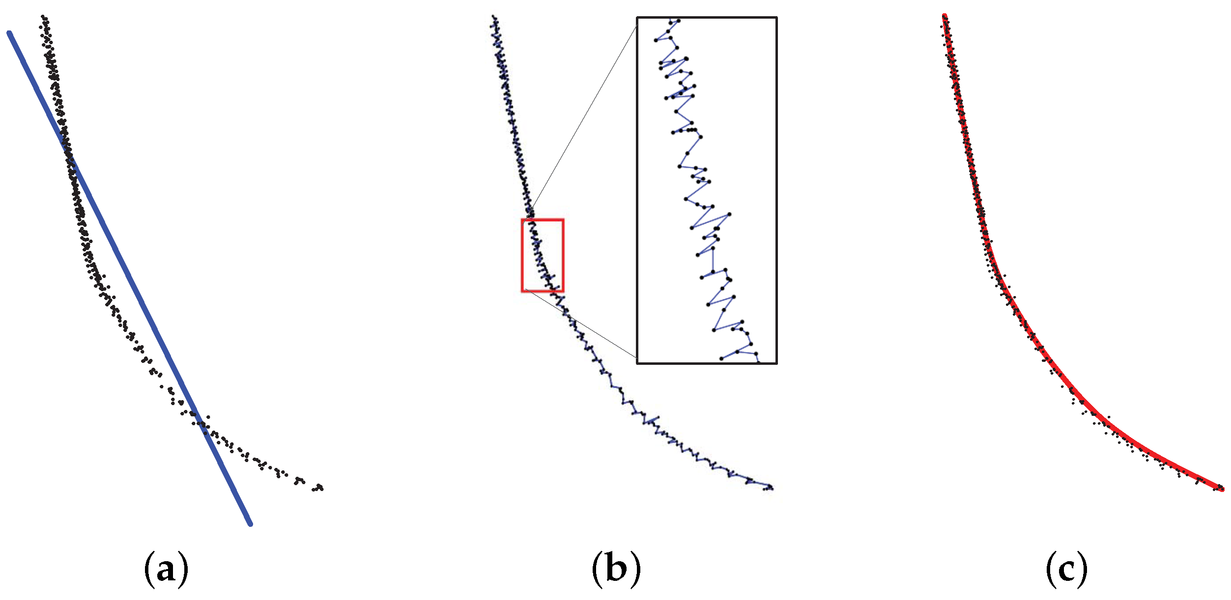
3.2.1. Centerline Generation from Point Cluster

There are many types of centerline generation algorithms for unorganised point clouds in the computer science community [30]. The point clusters generated by our algorithm represent nearly straight curves. The curve does not self-intersect, but is distorted by noise and outliers. Thus, we use the robust Lowess method to generate the centerline of the point cluster. The method uses residual analysis to overcome the problem caused by noise and outliers.

Figure 2a is a typical point cluster generated with our map inference method. In order to apply the robust Lowess algorithm, we need to pre-process the point cluster. First, we rotate the points to the new coordinate system computed by PCA. The abscissa is shown as the line in Figure 2a. We then sort the points in ascending order according to their x values in the new coordinate system and connect them to form an unsmooth curve, which is shown in Figure 2b. After these two steps, we can use robust Lowess to generate a smooth curve, as shown in Figure 2c. Finally, we rotate the curve back to the original coordinate system.

The general procedure of the robust Lowess method can be summarised as follows:

• Apply a locally-weighted linear least-squares regression for each point to smooth the curve.
• Calculate the residual for each point according to the smoothed curve.
• Compute the value of MAD to remove outliers and update local weights. The residuals of the outliers are more than 6-times that of the value of MAD.
• Smooth the curve as described in Step 1, again using the new weights.
• Repeat Steps 2 through 4 for a total of five iterations to obtain a smooth curve.

In the algorithm, the local linear regression for each point is performed on its k nearest neighbours, which is computed by their x values in the rotated coordinate system. We need to manually determine k for each cluster. Since the density (numbers of points in a fixed area) of raw GPS points varies over space, we use the average number of the points contained in a specified span $dSpan$ to estimate k: $k=dSpan/l\times n$, where l is the length of the line segment generated from the point cluster with PCA and n is the number of the points in the cluster. We fixed the $dSpan$ to 10 m according to experimental tests.

For each point cluster $c_i=\left\{p_{i,r}\right|r=1,2,\dots ,m\}$, we generate its centerline $l_i$: $l_i=\left\{v_{i,r^{\prime }}\right|r^{\prime }=1,2,\dots ,m^{\prime }\wedge m^{\prime }\le m\}$, where $v_{i,r^{\prime }}$ is the nodes that constitute the centerline. Due to outliers, the number of nodes ($m^{\prime }$) that constitute the centerline $l_i$ is less than or equal to the number of points (m) in cluster $c_i$. We can then estimate the corresponding ${\sigma }_i$ with the MAD formula, as shown in Equation (1).

$${\sigma }_i=1.4826\times \text{median}|dis(p_{i,r},l_i)-\text{median}\left(dis(p_{i,r},l_i)\right)|$$

(1)

where $dis(p_{i,r},l_i)=min\left\{dis(p_{i,r},v_{i,r^{\prime }})\right\},(r^{\prime }=1,2,\dots ,m^{\prime })$ is the distance from point $p_{i,r}$ to centerline $l_i$, $dis(p_{i,r},v_{i,r^{\prime }})$ is the Euclidean distance from point $p_{i,r}$ to node $v_{i,r^{\prime }}$, and 1.4826 is the scaling factor for normal distribution data. Although the distribution of point clusters does not strictly comply with the Gaussian distribution, we can obtain a reasonable estimation with the MAD formula.

3.2.2. Topological Relationship Construction between Clusters

According to Newson and Krumm [28], matching of GPS traces to the actual road map (i.e., map matching) is achieved through finding the most probable route that the vehicle visited based on the location of the vehicle measured by GPS. They modelled the map matching problem as an HMM, which is a Markov process with a set of hidden states and observations. Transitions from state to state are defined by transition probabilities. Each state has a probability distribution called the emission probability distribution over the possible observations. Given a sequence of observations, a sequence of hidden states can be generated by maximizing the overall probability.

In the context of map matching, the hidden states are road segments; and observations are the points measured by GPS. The transition probabilities provide the probabilities that the vehicle transitions from one segment to another; and the emission probability for a state over an observation denotes the probability that the vehicle actually visited the segment given the point (position of vehicle) measured by GPS.

In the HMM-based map matching algorithm proposed by Krumm et al. [28,31], they projected each point measured by GPS to its nearby road segments to generate a set of candidates for matching and calculated the emission probability based on the distance from the point to the projected point of each candidate. For a vehicle moving from one point to the next point (measured by GPS), a set of possible transitions from one road segment to another could then be generated. The transition probabilities for the segments are calculated according to the difference of two distances: (1) the Euclidean distance of the two GPS points; and (2) the shortest path length of the two projected points on road segments. Finally, they use the Viterbi algorithm to match the GPS trace generated by a vehicle with the path that had the maximum probability among all possible paths. The algorithm simultaneously considered the locations of GPS points and the topological relationship of the actual road map. This method is robust to noise.

The proposed method matches the raw GPS traces with the centerlines generated by point clusters to build the topological relationships between the point clusters. The hidden state is the centerline, and the observation is the point measured by GPS. The matching result also can be used to remove the redundant point clusters that are caused by noises.

The transition probabilities in our method provide the probability of a vehicle moving from one centerline $l_i$ (generated by $c_i$) to another centerline $l_j$ (generated by $c_j$). It is derived from the two point clusters $c_i$ and $c_j$, where $c_i=\left\{p_{i,r}\right|r=1,2,\dots ,m\}$, $c_j=\left\{p_{j,s}\right|s=1,2,\dots ,n\}$ and m and n are the sizes of the clusters. The sequences of the points are indicated by the raw GPS traces. Intuitively, if there are $m_{i,j}$ ($m_{i,j}\le m$) points in $c_i$ that have their next points contained in $c_j$, we define the transition probability for transitioning from state $l_i$ to $l_j$ as $\text{Pr}(l_i,l_j)=m_{i,j}/m$. Based on this definition, the sum of the non-zero transition probabilities $\text{Pr}(l_i,l_j)$ for transitioning from $l_i$ to all of the other possible $l_j$ is equal to 1; and we call the number of possible $l_j$ the out-degree $d\left(l_i\right)$ of $l_i$.

In experiments with actual GPS data, we observed two facts for some centerlines: (1) $\text{Pr}(l_i,l_i)\gg \text{Pr}(l_i,l_j)$, where $i\ne j$, which means that the transition probability for transitioning from centerline $l_i$ to itself is much bigger than transitioning from $l_i$ to others; and (2) $\text{Pr}(l_i,l_j)\gg \text{Pr}(l_r,l_s)$, where $d\left(l_i\right)\ll d\left(l_r\right)$ and $i\ne j$, $r\ne s$, which denotes that the transition probabilities for transitioning from lower out-degree centerlines are much larger than the transition probabilities for transitioning from higher out-degree centerlines. In order to avoid the preference for matching GPS traces with low out-degree centerlines, we refined the transition probabilities $\text{Pr}(l_i,l_j)$ to be independent of the out-degree of centerlines by introducing a weight factor ω. The weight factor is derived from the out-degree of centerlines. The results based on this setting are more reasonable. The refining steps are as follows:

• For a point cluster $c_i\in C$, obtain the number $m^{\prime }$ of the points included in $c_i$ that their successive points are not included in $c_i$.
• For a point cluster $c_j\in C$, obtain the number $m_{i,j}$ of the points included in $c_i$ that have their successive points in $c_j$ ($i\ne j$).
• Compute the transition probability for transitioning from centerline $l_i$ to $l_j$, $\text{Pr}(l_i,l_j)=m_{i,j}/m^{\prime }$.
• Repeat Steps 2 and 3, computing transition probabilities for transiting from the $l_i$ to all possible $l_j$.
• Define $\text{Pr}(l_i,l_i)=\text{max}\left(\text{Pr}(l_i,l_j)\right)$, ($i\ne j$).
• Repeat Steps 1 to 5, computing the non-zero transition probabilities of all centerlines $l_i\in L$.
• Find minimum out-degree $d_{min}$ among all of the out-degrees of all centerlines $l_i\in L$.
• Update transition probabilities as $\text{Pr}(l_i,l_j)={\omega }_i\times \text{Pr}(l_i,l_j)$, where $l_i\in L$, $l_j\in L$ ${\omega }_i$ is a weight factor, and ${\omega }_i=d\left(l_i\right)/d_{min}$.

The emission probability for a particular point $p_t$ measured by GPS at time t associated with a nearby centerline $l_i$, denoted by $\text{Pr}\left(l_i\right|p_t)$, gives the likelihood that $p_t$ was observed from $l_i$. It indicates the probability that the vehicle visited the centerline $l_i$ at time t given the measurement $p_t$. We calculate the emission probability based on the assumption that the distance distribution of points to the centerline complies with Gaussian distribution $G\sim (\mu ,{\sigma }^2)$. For each point of raw GPS traces, the probabilities are estimated with Equation (2):

$$\text{Pr}\left(l_i\right|p_t)=\frac{1}{\sqrt{2\pi }\sigma }{e}^{-0.5{\left(\frac{dis(p_t,l_i)}{\sigma }\right)}^2}$$

(2)

where $dis(p_t,l_i)=\text{min}\left\{dis(p_t,v_{i,r^{\prime }})\right|v_{i,r^{\prime }}\in l_i\}$ is the distance from point $p_t$ to centerline $l_i$.

Variance σ is estimated in the centerline generation procedure. After computing ${\sigma }_i$ for each point cluster $c_i$, we use $\underset{i}{max}{\sigma }_i$ as σ to estimate the emission probabilities. In practice, we find up to 10 matched centerline candidates for each point. If the $dis(p_t,l_i)$ is greater than $6\times \sigma$, the emission probability is close to 0, and we do not consider $l_i$ as a candidate for matching with $p_t$. The emission probability $\text{Pr}\left(l_i\right|p_t)$ of point $p_t$ is normalised by scaling to [0, 1].

After initializing the transition probabilities and emission probabilities, we use the Viterbi map matching algorithm [28,32] to match raw GPS traces with generated centerlines to find the most probabilistic path that vehicles visited. The path with the highest probability indicates the connectivity between clusters. Clusters that do not match with any raw trace are treated as noise.

3.2.3. Point Cluster Grouping

A set of routes $O=\left\{o_i\right|i=1,2,\dots ,N\}$ is obtained by matching raw GPS traces with centerlines, where N is the number of routes, which corresponds to the number of traces. Each route $o_i$ is produced by matching a trace $t{r}_i=\left\{p_{i,r}\right|r=1,2,\dots ,n\}$ with centerlines. Thus, $o_i$ consists of a set of centerlines, $o_i=\{l_{i_1},l_{i_2},\dots ,l_{i_n}\}$, where $l_{i_r}$ is matched with point $p_{i,r}$ of trace $t{r}_i$. Since we know a vehicle moves from point $p_{i,r}$ to the next point, $p_{i,r+1}$, we can infer that centerlines $l_{i_r}$ and $l_{i_{r+1}}$ are topologically connected. In the next step, we employ the geometric positions of these two centerlines to determine if they can be grouped.

The concept of a stroke is that a curve can be drawn in one smooth movement [9]. It is derived from the principle of good continuation, which indicates that elements that follow similar directions tend to be grouped together. Using the stroke concept, we group point clusters to generate smooth curves to the farthest possible extent. For two point clusters $c_i$ and $c_j$ that produce two topologically-connected curves $l_i$ and $l_j$, respectively, we temporarily group $c_i$ and $c_j$ to obtain a new point cluster $c_g$ and generate a new centerline $l_g$ by $c_g$. If $l_g$ is spatially near to $l_i$ and $l_j$, we make the grouping permanent; otherwise, we retain $c_i$ and $c_j$. Based on this idea, we propose a new point cluster grouping algorithm, as demonstrated in Algorithm 3.

Algorithm 3: Point clusters grouping algorithm.
	Input: TwoPointClusters $c_i$, and $c_j$, β
	Output: NewPointClusters
1	calculate the difference of mean orientations $DoOs$ by points in $c_i$ and $c_j$;
2	if $DoOs>\beta$ then
3	$\lfloor$ return the two clusters $c_i$ and $c_j$;
4	generate the centerlines $l_i$ and $l_j$ for point cluster $c_i$ and $c_j$ by robust Lowess;
5	estimate the errors ${\sigma }_i$ and ${\sigma }_j$ by MAD for $c_i$ and $c_j$;
6	generate a new centerline $l_g$ by $c_g=c_i\cup c_j$;
7	$\forall v_{i,r^{\prime }}\in l_i$ find the $dis(v_{i,r^{\prime }},l_g)=min\left\{dis(v_{i,r^{\prime }},v_{g,t})\right|v_{g,t}\in l_g\}$ as the distance set $Dis(l_i,l_g)$;
8	$\forall v_{j,s^{\prime }}\in l_j$ find the $dis(v_{j,s^{\prime }},l_g)=min\left\{dis(v_{j,s^{\prime }},v_{g,t})\right|v_{g,t}\in l_g\}$ as the distance set $Dis(l_j,l_g)$;
9	sort distances in $Dis(l_i,l_g)$ and $Dis(l_j,l_g)$ as $Di{s}_s(l_i,l_g)$ and $Di{s}_s(l_j,l_g)$ in descending order;
10	compute the mean distance of the distances from the beginning to the α-quantile in the set $Di{s}_s(l_i,l_g)$ and $Di{s}_s(l_j,l_g)$ as $di{s}_{\alpha }(l_i,l_g)$ and $di{s}_{\alpha }(l_j,l_g)$;
11	if $di{s}_{\alpha }(l_i,l_g)$+$di{s}_{\alpha }(l_j,l_g)>6\times ({\sigma }_i+{\sigma }_j)$ then
12	$\lfloor$ return the two clusters $c_i$ and $c_j$;
13	else
14	$\lfloor$ return the new grouped cluster $c_g$;

First, we use the difference of the mean orientations of two point clusters $c_i$ and $c_j$ to determine if centerlines $l_i$ and $l_j$ produced by $c_i$ and $c_j$ connect smoothly to each other (Lines 1 to 3). According to Jiang et al. [33], the threshold of the deflection angle for generating a stroke from road segments with a range of [30°, 75°] produces stable outcomes. The deflection angle is the angle between two connected road segments.

In our method, we intend to generate a longer nearly straight curve, $l_g$, from point cluster $c_g$ produced by grouping point clusters $c_i$ and $c_j$. Similar to the idea of stroke generation, if the difference of the mean orientations of $c_i$ and $c_j$ is larger than a predefined threshold β, we assume $c_i$ and $c_j$ cannot be grouped. We set β to 60° based on the experimental testing. However, in order to group point clusters with smaller differences of orientations well ahead of the point clusters with larger differences of orientations, we employ a progressive method: we apply Algorithm 3 to the set of point cluster C that begins with a small β (i.e., 10°) and iteratively run Algorithm 3 by increasing β in a step size (i.e., 10°) until it reaches 60°.

If the difference of mean orientations of $c_i$ and $c_j$ is smaller than β, we use the geometric position of points in $c_i$ and $c_j$ to determine if the two point clusters can be grouped or not. Figure 3 provides an illustration of the grouping of two point clusters. The black dashed lines in Figure 3 give the buffer regions for $l_i$ and $l_j$ with radii of $6{\sigma }_i$ and $6{\sigma }_j$, respectively. By assuming that $c_i$ and $c_j$ can be grouped, we obtain the point cluster $c_g$ and generate centerline $l_g$ as the red solid line in Figure 3. If $l_g$ is in the union of the buffer regions of $l_i$ and $l_j$, we can make the grouping of $c_i$ and $c_j$ permanent. According to Equation (1), ${\sigma }_i$ and ${\sigma }_j$ are estimated based on $c_i$, $l_i$ and $c_j$, $l_j$. We implement the grouping of $c_i$ and $c_j$ by using the distances from the points of $l_i$ and $l_j$ to the points of $l_g$ as a metric. The procedure is shown as Lines 4 to 14 in Algorithm 3.

For each node $v_{i,r^{\prime }}\in l_i$, we find the nearest node $v_{g,t}\in l_g$ according to their Euclidean distance $dis(v_{i,r^{\prime }},v_{g,t})$ as the distance $dis(v_{i,r^{\prime }},l_g)$ from node $v_{i,r^{\prime }}$ to the centerline $l_g$. A distance set $Dis(l_i,l_g)=\left\{dis(v_{i,r^{\prime }},l_g)\right|r^{\prime }=1,2,\dots ,m^{\prime }\}$ can then be obtained by computing distances from all nodes of $l_i$ to centerline $l_g$, where $m^{\prime }$ is the number of nodes in $l_i$. We sort the distances in $Dis(l_i,l_g)$ as $Di{s}_s(l_i,l_g)$ in descending order and obtain the mean distance from the beginning to the α-quantile in $Di{s}_s(l_i,l_g)$ as the α-quantile mean distance $di{s}_{\alpha }(l_i,l_g)$ from centerline $l_i$ to $l_g$. The α-quantile mean distance $di{s}_{\alpha }(l_j,l_g)$ from $l_j$ to $l_g$ can also be obtained by the same procedure. Finally, if the sum of the two α-quantile mean distances is smaller than or equal to $6\times ({\sigma }_i+{\sigma }_j)$, we group the two point clusters $c_i$ and $c_j$ to obtain $c_g$. The α-quantile mean distance represents the deviation from the two original centerlines to the new centerline that produced by the two grouped clusters. $di{s}_{\alpha }(l_i,l_g)+di{s}_{\alpha }(l_j,l_g)\le 6\times ({\sigma }_i+{\sigma }_j)$ means the new centerline is in the union of the two buffer regions of $l_i$ and $l_j$. According to the experimental testing, we set the α to a small value (i.e., 0.02).

Another issue is that the sampling rates of the raw GPS traces are not consistent. Two topologically-connected clusters may not be spatially near to each other. We define the distance between two clusters as in Equation (3). If the distance between two clusters $dis(c_i,c_j)$ is greater than a threshold (i.e., 100 m), they cannot be grouped. In the experiment of sparsely-sampled GPS traces, we found that the most probabilistic path could not discover the relationship between two adjacent clusters. Thus, as a final step of cluster grouping, we find the clusters for grouping according to the distance between them. If the distance between two clusters is less than or equal to a threshold (i.e., 100 m), we apply the grouping algorithm with an angle threshold β equal to 60° to these two clusters.

$$dis(c_i,c_j)=\underset{p_{i,r}\in c_i}{min}(\underset{p_{j,s}\in c_j}{min}dis(p_{i,r},p_{j,s}))$$

(3)

4. Experiments

We used two datasets to test our algorithm. The dataset collected in Chicago, USA (Dataset 1), consists of densely-sampled traces; and the other dataset collected in Wuhan, China (Dataset 2), consists of sparsely-sampled traces. The characteristics of the two datasets are described below:

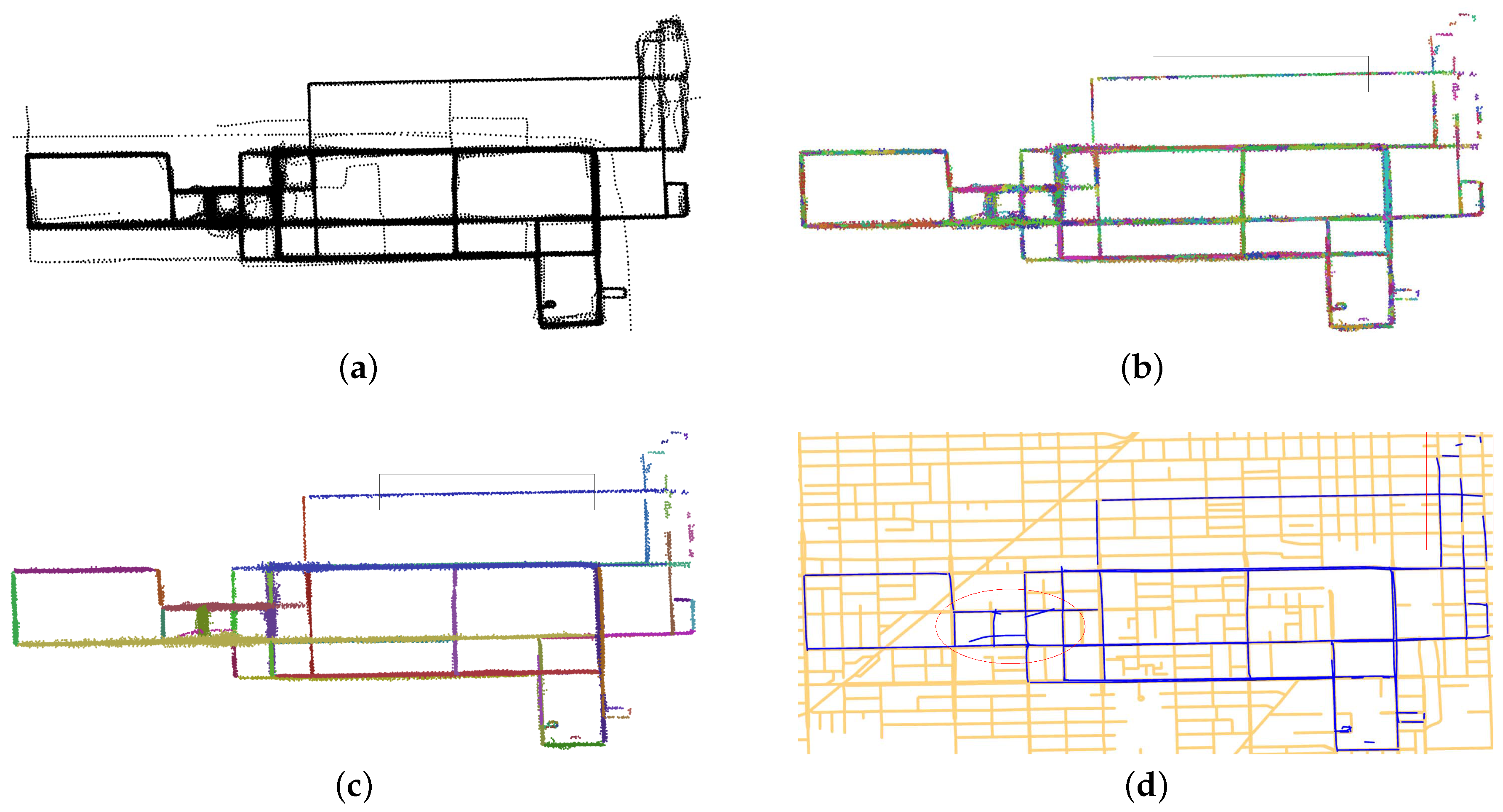
• The Chicago dataset was GPS traces from a bus serving the University of Illinois at Chicago campus [23]. The dataset covered an area of 3.8 km × 2.4 km, with the sampling rates varying from 1 s to 29 s (with a mean of 3.61 s and standard deviation of 3.67 s). The distances between two consecutive points ranged from 19.97 m to 96.6 m (with a mean of 24.4 m and standard deviation of 3.31 m). There were about 118,000 points.
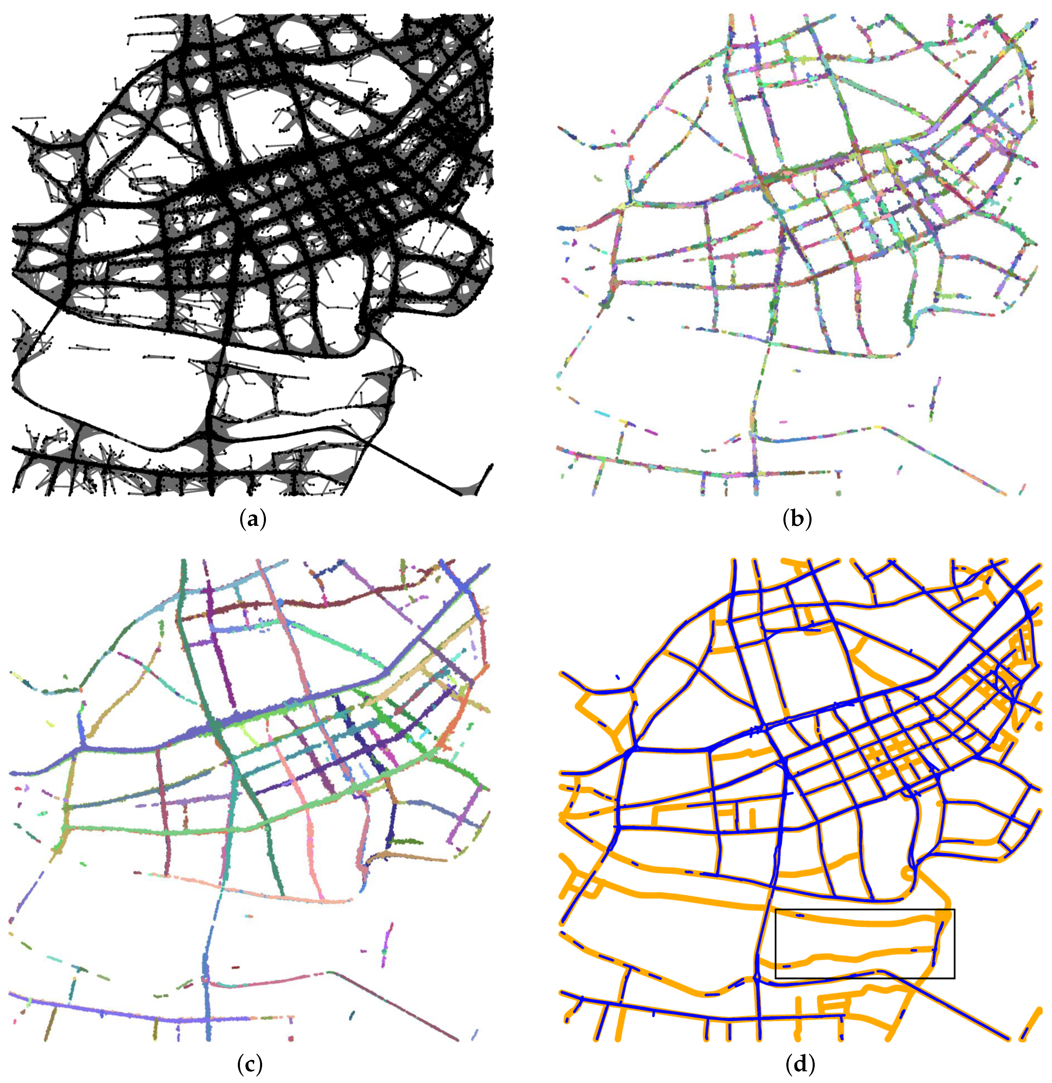
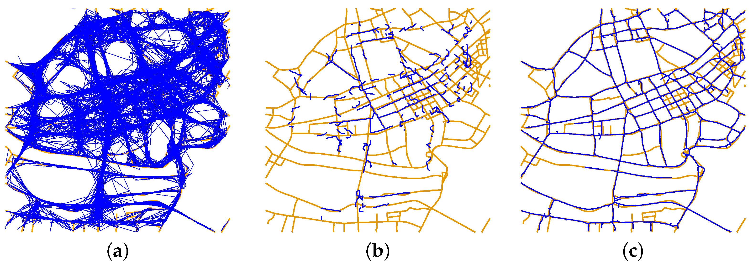
• The Wuhan dataset was GPS traces collected by taxis. The dataset covered an area of 4.8 km × 5.5 km, with the sampling rates varying from 1 s to 81 s (with a mean of 37.42 s and standard deviation of 17.66 s). The distances between two consecutive points ranged from 0 m to 496.255 m (with a mean of 218.84 m and standard deviation of 140.38 m). There were about 350,000 points.

Figure 4a shows the raw GPS traces of the Chicago dataset displayed as points. We applied our progressive DBSCAN algorithm with an orientation constraint to the dataset and obtained the 2D GPS points segmentation results, as shown Figure 4b. A total of 1099 point clusters were obtained, and those that were spatially adjacent to each other are shown in different colours. In Figure 4b, we can visually detect that the clusters in the rectangle could be grouped to produce a nearly straight curve, due to their similar orientations and spatial adjacency. The reason for generating clusters with similar orientations are the following: (1) we applied the segmentation algorithm beginning with a strong constraint (α for finding neighbours of a point is 1°); and (2) orientations computed by two consecutive points were inaccurate due to the noise of GPS points and the sampling rate.

We then matched raw GPS traces with the centerlines that were generated by the point clusters to construct the topological relationship between clusters. Clusters that were topologically connected were grouped according to their geometric position. As the final step of point clusters’ progressive grouping procedure, we also used the HMM-based map matching method to filter the clusters. If the centerline $l_i$ was matched with only two (or less) raw GPS traces, we regarded $l_i$ to be generated by noise and removed the corresponding point cluster $c_i$.

Figure 4c shows the point cluster grouping results. Fifty-five clusters were obtained. A comparison of Figure 4b,c shows that the point clusters in the rectangle have been grouped by our algorithm. In fact, spatially-adjacent clusters with similar orientations were grouped properly.

As a final step, we used the robust Lowess algorithm to generate centerlines from the grouped point clusters. The inferred road map (blue lines) was overlapped with the ground truth map (light yellow lines) in Figure 4d. According to Figure 4d, the inferred road segments in the rectangle did not represent the ground truth map well: the roads were not frequently visited by the GPS-equipped vehicles; therefore, there was a lack of sufficient points to recover the roads with our algorithm. In the ellipse shown in Figure 4d, some spurious road segments were generated. As can be observed in Figure 4a, GPS points in this area were noisy, and the accumulation of the noise produced the spurious road segments.

We applied the same procedure to the Wuhan dataset. Figure 5a shows the preprocessed GPS traces (grey lines) overlapped with the corresponding points (black points). According to this figure, the sparsely-sampled GPS traces could not align well with the real position of the vehicles, especially for the traces near the road network’s intersections. We then used our segmentation algorithm to generate point clusters, as shown as Figure 5b. Due to the inaccuracy of the GPS points’ orientations, 4970 clusters were generated. After grouping, the 216 clusters shown in Figure 5c were obtained. Finally, we generated the centerlines of the road network with the robust Lowess algorithm. The centerlines are shown as blue lines in Figure 5d, and the yellow lines represent the ground truth map. Figure 5d indicates that some road segments (e.g., road segments in the rectangular area) could not be recovered due to an insufficient number of GPS points.

We compare our map inference method with four typical methods, including a hybrid map inference pipeline [23], a clustering-based method [12], a KDE-based method [20] and a trace merging-based method [15] using the Wuhan dataset. The results are shown in Figure 6. Figure 6a shows the roads generated by Edelkamp and Schrödl’s method. Their method cannot generate road centerlines for these traces. The reason is that the points’ orientations of sparsely-sampled GPS traces are inaccurate, and hence, the cluster seeds cannot be grouped together. We used 3000 traces for the method (the total number of the traces in Wuhan dataset is 12,832). According to Figure 6a, the 3000 traces cover the road network on the ground truth map. Figure 6b shows the road network generated by Biagioni and Eriksson’s method. We applied the full number of traces to this method. However, the algorithm failed at the step of collapsing nodes into intersections. We then applied the method to 3000 traces, as in Figure 6b. Due to the sparse sampling rate, many roads could not be recovered by the algorithm. Figure 6c shows the road network generated by Davies’ method with the full number of traces in the Wuhan dataset. The method is robust to the sampling rate, and we compare our method to this method in the next section. We also evaluated Cao and Krumm’s method using the Wuhan dataset. However, due to the sparse sampling rate, the algorithm did not converge, and adjacent traces were not merged.

Thus far, we have only compared the inferred road centerlines to the ground truth maps to qualitatively evaluate our map inference algorithm. In the next section, we present a quantitative evaluation for the geometric accuracy of our map inference algorithm.

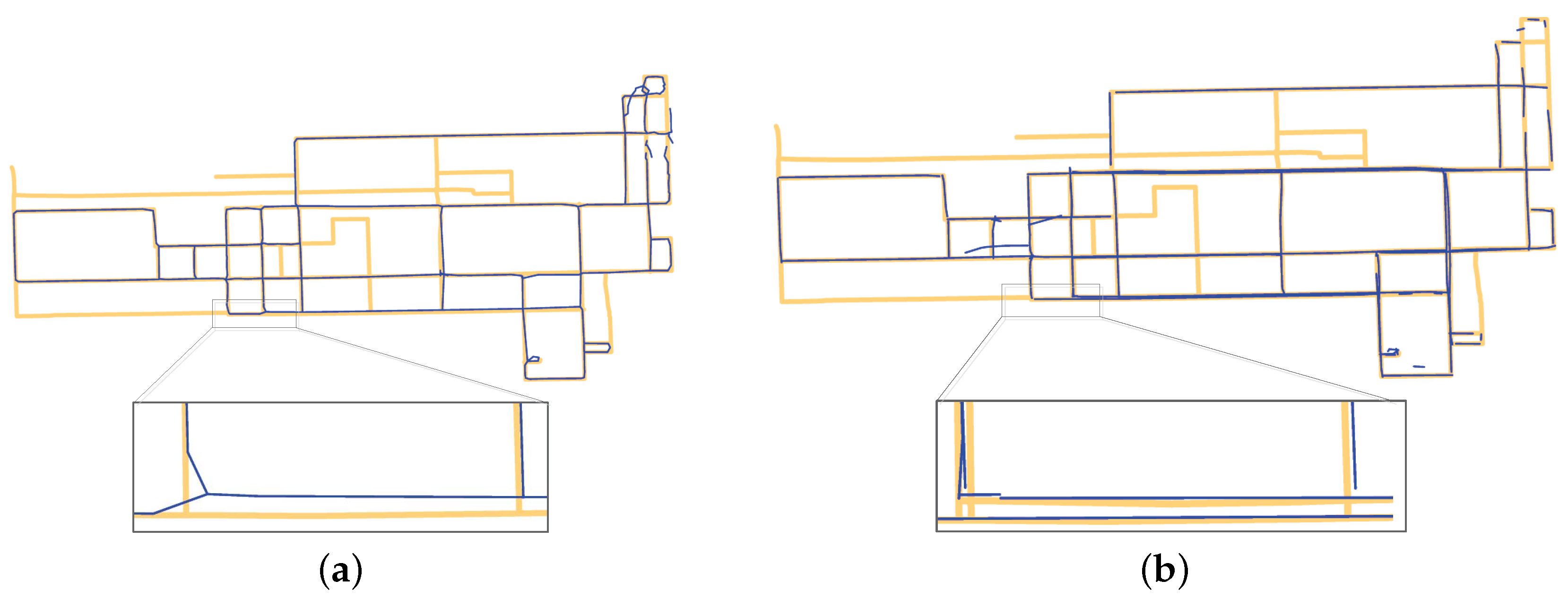
5. Evaluation

Several quantitative evaluation methods for the accuracy of the geometry and topology of inferred road maps have recently been proposed. Liu et al. [19] performed their quantitative evaluation by measuring the recall and precision of the roads on the inferred map (M) with respect to the roads on the ground truth map ($Truth$). The recall denoted the fraction of roads on the ground truth map that were retrieved, and the precision was the fraction of roads on the inferred map that were relevant. They used distance and orientation as constraints to match the roads of the two maps with each other by nearest distance and to determine the true positive length $tp=M\cap Truth$ by the matched proportion. The recall, precision and F-measure were then calculated as follows: $recall=tp/\left|\right|Truth\left|\right|$, $precision=tp/\left|\right|M\left|\right|$, and $F-measure=(2\times precision\times recall)/(precision+recall)$, where $\left|\right|.\left|\right|$ measures the total length of the road segments in the corresponding set. Their method evaluated the geometric accuracy of the inferred map.

Biagioni and Eriksson [23] introduced a new method to measure the geometric and topological similarities of the inferred and ground truth maps at the same time. They resampled the two types of maps and placed holes on the ground truth map and marbles on the inferred map. They then matched marbles with holes by the distances between them and counted the unmatched marbles and empty holes. The accuracy of the inferred map with respect to the ground truth map was quantified by the spurious marbles and empty holes.

Karagiorgou and Pfoser [25] used the shortest path to measure the similarity of the inferred and ground truth maps. They simultaneously placed origins and destinations on the two maps and computed the shortest path between them to obtain two sets of shortest paths. They applied discrete Fréchet distance and average vertical distance to compare the similarity of the two sets of shortest paths to quantitatively measure the inferred map. Their method focuses on the connectivity of the road segments.

Ahmed et al. [11] proposed a path-based distance measure for road map comparison. They used the distances between two paths (i.e., maps) that were calculated based on the Hausdorff distance to measure the distances between two road networks. Their method took into account the structural and spatial properties of the road map.

We use the method proposed by Liu et al. [19] to evaluate the geometric accuracy of the inferred road maps. The details of the geometry evaluation method can be described as follows:

• Place points on the roads of the ground truth and inferred maps with equal intervals (i.e., 1 m).
• Compute the orientations of all points by their connections (modulo 180°).
• Match the sampled points on the inferred map with the ground truth map by nearest distance matching under the constraint of the orientation. The difference of orientations of two points that are matched with each other is no more than 60°.
• Use different distance thresholds to determine the best match proportion.

The ground truth map (yellow lines) and inferred map (blue lines) of the Chicago dataset were overlapped, as shown in Figure 7. Figure 7a presents the road map generated by Biagioni and Eriksson’s algorithm [23]. We manually selected the roads of the ground truth map that were actually visited by vehicles according to the raw GPS traces. Each road was represented by one centerline, since their algorithm did not separate the centerlines with opposite directions for a bidirectional road. Figure 7b is the road map generated by our method. As shown in detail, we generated two centerlines for the opposite directions of a bidirectional road. The corresponding roads of the ground truth map also had two centerlines.

The total length of the roads on the ground truth map in Figure 7a,b are 32.89 km and 41.1 km, respectively. The total length of the inferred road map in Figure 7a (Biagioni and Eriksson’s method) and Figure 7b (our method) was 24.50 km and 30.9 km, respectively. In Figure 7b, we infer two centerlines for the bi-directional roads, which are also represented by two centerlines on the ground truth map. However, all of the roads in Figure 7a are represented by single centerlines. This is the reason that the total length of the roads on the ground truth map and inferred road map in Figure 7b is longer than the roads in Figure 7a. We evaluate the two inferred road maps by different matching thresholds of distance, where the results are shown in

Table 1. Matching results of Biagioni and Eriksson’s method on the Chicago dataset.

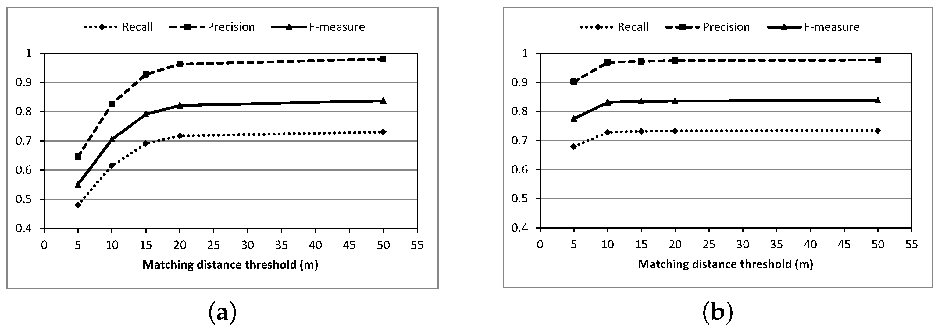
Matching Threshold of Distance (m)	Length of Well-matched Roads (km)	Recall	Precision	F-measure
5	15.11	0.459	0.617	0.526
10	20.22	0.615	0.826	0.705
15	22.71	0.690	0.927	0.791
20	23.57	0.717	0.962	0.821
50	24.01	0.730	0.980	0.837

and

Table 2. Matching results of our method on the Chicago dataset.

Matching Threshold of Distance (m)	Length of Well-matched Roads (km)	Recall	Precision	F-measure
5	27.93	0.679	0.902	0.775
10	29.96	0.728	0.968	0.831
15	30.09	0.732	0.972	0.835
20	30.13	0.733	0.974	0.836
50	30.19	0.734	0.975	0.838

. In Table 1 and Table 2, the length of well-matched roads is the total length of roads on the ground truth map (or the inferred map) that were matched with roads on the inferred map (or the ground truth map), given the matching threshold of distance.

Figure 8 presents the plots of the recall, precision and F-measure of the two methods. Figure 8a shows that the values of the recall, precision and F-measure criteria of Biagioni and Eriksson’s method [23] increase as the matching threshold increase from 5 m to 20 m and became constant after the threshold reached 20 m. Figure 8b demonstrates that the values of these three criteria did not change much with our method after reaching the matching threshold of 10 m. The values of the criteria of our method were larger than the values of Biagioni and Eriksson’s method when the matching threshold was smaller than 20 m. These results indicate that the road map inferred by our method has better accuracy in terms of the geometry. In addition, Biagioni and Eriksson demonstrated using the same dataset [23] that, in terms of geometry, their method outperformed the existing map inference methods, i.e., clustering-based methods, trace merging-based methods and KDE-based methods.

The ground truth and inferred maps for Dataset 2 (Wuhan dataset) are displayed in Figure 5d. We separated the centerlines with opposite directions for bidirectional roads; however, the ground truth map only had one centerline for each road segment. Thus, all sampled points of the ground truth map could be matched with two points of the inferred roads. The total length of roads on the ground truth map in Figure 5d is 117.67 km, and the total length of the roads inferred by our method was 148.38 km. The matching results are shown in

Table 3. Matching results of our method for the Wuhan dataset.

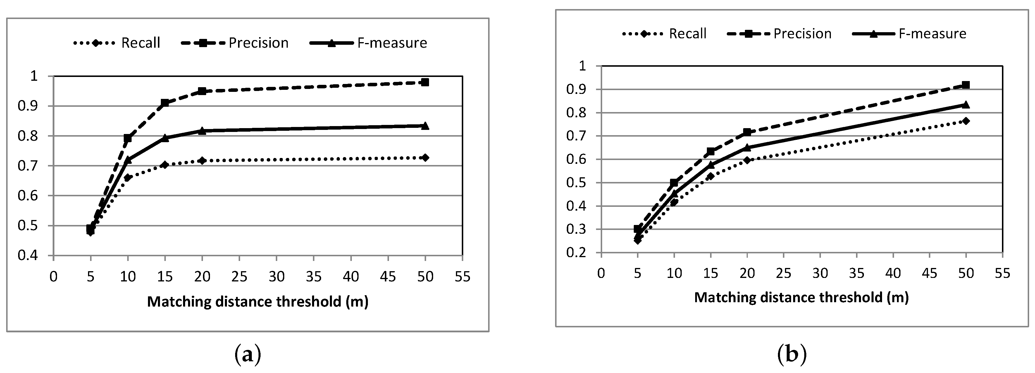
Matching Threshold of of Distance (m)	Length of Well-Matched Roads (km)	Length of Correctly Inferred Roads (km)	Recall	Precision	F-measure
5	56.14	72.78	0.477	0.490	0.484
10	77.61	117.48	0.660	0.792	0.720
15	82.74	135.00	0.703	0.910	0.793
20	84.37	140.75	0.717	0.949	0.817
50	85.52	145.26	0.727	0.979	0.834

. The length of well-matched roads represents the total length of roads on the ground truth map that matched with roads on the inferred map, given the matching threshold of distance. The length of the correctly inferred roads is the total length of roads on the inferred map that matched with roads on the ground truth map, given the matching threshold of distance. Since the total length of roads on the inferred road map was larger than the total length of roads on the ground truth map, we modified the standard formula of recall and precision as follows: $recall=\left|\right|wellmatchedroads\left|\right|/\left|\right|Truth\left|\right|$, and $precision=\left|\right|correctlyinferredroads\left|\right|/\left|\right|M\left|\right|$.

Table 4. Matching results of Davies’ method for the Wuhan dataset.

Matching Threshold of of Distance (m)	Length of Well-Matched Roads (km)	Recall	Precision	F-measure
5	29.51	0.251	0.301	0.274
10	48.87	0.415	0.499	0.453
15	62.06	0.527	0.633	0.576
20	70.05	0.595	0.715	0.65
50	89.92	0.764	0.918	0.834

shows the matching results of the road network generated by Davies’ method (Figure 6c). The total length of the inferred roads in Figure 6c is 97.97 km.

Figure 9 displays the graphical plots of recall, precision and F-measure for the sparsely-sampled Wuhan dataset (Dataset 2). Figure 9a is the plot of our method; and Figure 9b is the plot of Davies’ method. According to Figure 9a, the precision is greater than 0.9, when the matching threshold of distance is larger than 15 m. Therefore, we conclude that our method can infer a road map from sparsely-sampled GPS traces with high geometric accuracy. When the threshold is equal to 5 m, the precision is found to be less than 0.5, because we generated two centerlines for the bidirectional roads and the ground truth map only used one centerline to represent bidirectional roads. On comparing Figure 9a,b, we conclude that the road network generated by our method has a better geometric accuracy than the road network inferred by Davies’ method.

6. Conclusions

We have proposed a new segmentation and grouping framework for road map inference from GPS traces. The key aspect is the partitioning of the whole points of the GPS traces into clusters that represent nearly straight curves to recover the road map. In summary, our method has the capability to deal with both densely- and sparsely-sampled GPS traces. According to the experimental and evaluation results, we can conclude that our method performs well in terms of the geometric accuracy. The framework we proposed is open and flexible. We can develop a more sophisticated 2D point cloud segmentation algorithm to replace the current one, thereby further improving the overall performance of the proposed method. We can also use other types of skeletonisation algorithms that are more robust to noise to generate the centerlines of the point clusters.

In this research, we used two consecutive points to estimate the orientations of points. However, noise and sparse sampling considerably affect the accuracy of orientation estimation. In future work, we plan to integrate the connection between points and the point cloud distribution to estimate orientations to improve the performance of our algorithm. The method is designed to generate nearly straight curves to recover the road network. However, not all roads are straight. In future work, we will simulate curves with a sequence of line segments to infer winding roads from GPS traces. In addition, we need to process the intersections of the centerlines to generate the graph model of the road network.

References

- Wang, Y.; Liu, X.; Wei, H.; Forman, G.; Chen, C.; Zhu, Y. CrowdAtlas: Self-Updating maps for cloud and personal use. In Proceedings of the 11th Annual International Conference on Mobile Systems, Applications, and Services, Taipei, Taiwan, 25–28 June 2013; pp. 27–40.
- Guo, T.; Iwamura, K.; Koga, M. Towards high accuracy road maps generation from massive GPS traces data. In Proceedings of the 2007 IEEE International Geoscience and Remote Sensing Symposium, Barcelona, Spain, 23–28 July 2007.
- Fernandes, R.; Premebida, C.; Peixoto, P.; Wolf, D.; Nunes, U. Road detection using high resolution LiDAR. In Proceedings of the Vehicle Power and Propulsion Conference (VPPC), Coimbra, Portugal, 27–30 October 2014; pp. 1–6.
- Hillel, A.B.; Lerner, R.; Levi, D.; Raz, G. Recent progress in road and lane detection: A survey. Mach. Vis. Appl. 2014, 25, 727–745. [Google Scholar] [CrossRef]
- Krumm, J.; Davies, N.; Narayanaswami, C. User-generated content. IEEE Pervasive Comput. 2008, 7, 10–11. [Google Scholar] [CrossRef]
- Li, J.; Qin, Q.; Han, J.; Tang, L.-A.; Lei, K.H. Mining trajectory data and geotagged data in social media for road map inference. Trans. GIS 2015, 19, 1–18. [Google Scholar] [CrossRef]
- Schrödl, S.; Wagstaff, K.; Rogers, S.; Langley, P.; Wilson, C. Mining GPS traces for map refinement. Data Min. Knowl. Discov. 2004, 9, 59–87. [Google Scholar] [CrossRef]
- Lou, Y.; Zhang, C.; Zheng, Y.; Xie, X.; Wang, W.; Huang, Y. Map-Matching for low-sampling-rate GPS trajectories. In Proceedings of the 17th ACM SIGSPATIAL International Conference on Advances in Geographic Information Systems, Seattle, DC, USA, 4–6 November 2009; pp. 352–361.
- Thomson, R.C.; Brooks, R. Exploiting perceptual grouping for map analysis, understanding and generalization: The case of road and river networks. In Graphics Recognition Algorithms and Applications; Springer: Berlin, Germany, 2002; pp. 148–157. [Google Scholar]
- Biagioni, J.; Eriksson, J. Inferring road maps from global positioning system traces: Survey and comparative evaluation. Transp. Res. Record: J. Transp. Res. Board 2012. [Google Scholar] [CrossRef]
- Ahmed, M.; Karagiorgou, S.; Pfoser, D.; Wenk, C. A comparison and evaluation of map construction algorithms using vehicle tracking data. GeoInformatica 2015, 19, 601–632. [Google Scholar] [CrossRef]
- Edelkamp, S.; Schrödl, S. Route planning and map inference with global positioning traces. In Computer Science in Perspective; Springer: Berlin, Germany, 2003; pp. 128–151. [Google Scholar]
- Agamennoni, G.; Nieto, J.I.; Nebot, E.M. Technical Report: Inference of Principal Road Paths Using GPS Data; The University of Sydney, Australian Centre for Field Robotics: Sydney, Australia, 2010. [Google Scholar]
- Agamennoni, G.; Nieto, J.I.; Nebot, E.M. Robust inference of principal road paths for intelligent transportation systems. IEEE Trans. Intell. Transp. Syst. 2011, 12, 298–308. [Google Scholar] [CrossRef]
- Cao, L.; Krumm, J. From GPS traces to a routable road map. In Proceedings of the 17th ACM SIGSPATIAL International Conference on Advances in Geographic Information Systems, Seattle, DC, USA, 4–6 November 2009; pp. 3–12.
- Wang, J.; Rui, X.; Song, X.; Tan, X.; Wang, C.; Raghavan, V. A novel approach for generating routable road maps from vehicle GPS traces. Int. J. Geogr. Inf. Sci. 2015, 29, 69–91. [Google Scholar] [CrossRef]
- Niehoefer, B.; Burda, R.; Wietfeld, C.; Bauer, F.; Lueert, O. GPS community map generation for enhanced routing methods based on trace-collection by mobile phones. In Proceedings of the 2009 First International Conference on Advances in Satellite and Space Communications (SPACOMM 2009), Colmar, France, 20–25 July 2009; pp. 156–161.
- Chen, D.; Guibas, L.J.; Hershberger, J.; Sun, J. Road network reconstruction for organizing paths. In Proceedings of the Twenty-First Annual ACM-SIAM Symposium on Discrete Algorithms. Society for Industrial and Applied Mathematics, Philadelphia, PA, USA, 17–19 January 2010; pp. 1309–1320.
- Liu, X.; Biagioni, J.; Eriksson, J.; Wang, Y.; Forman, G.; Zhu, Y. Mining large-scale, sparse GPS traces for map inference: Comparison of approaches. In Proceedings of the 18th ACM SIGKDD International Conference on Knowledge Discovery and Data Mining, Beijing, China, 12–16 August 2012; pp. 669–677.
- Davies, J.J.; Beresford, A.R.; Hopper, A. Scalable, distributed, real-time map generation. IEEE Pervasive Comput. 2006, 5, 47–54. [Google Scholar] [CrossRef]
- Chen, C.; Cheng, Y. Roads digital map generation with multi-track GPS data. In Proceedings of the 2008 International Workshop on Education Technology and Training & 2008 International Workshop on Geoscience and Remote Sensing (ETT and GRS), Shanghai, China, 21–22 December 2008; pp. 508–511.
- Shi, W.; Shen, S.; Liu, Y. Automatic generation of road network map from massive GPS, vehicle trajectories. In Proceedings of the 12th International IEEE Conference on Intelligent Transportation Systems, Louis, MO, USA, 4–7 October 2009; pp. 1–6.
- Biagioni, J.; Eriksson, J. Map inference in the face of noise and disparity. In Proceedings of the 20th International Conference on Advances in Geographic Information Systems, Redondo Beach, CA, USA, 6–9 November 2012; pp. 79–88.
- Fathi, A.; Krumm, J. Detecting road intersections from GPS traces. In Geographic Information Science; Springer: Berlin, Germany, 2010; pp. 56–69. [Google Scholar]
- Karagiorgou, S.; Pfoser, D. On vehicle tracking data-based road network generation. In Proceedings of the 20th International Conference on Advances in Geographic Information Systems, Redondo Beach, CA, USA, 6–9 November 2012; pp. 89–98.
- Qiu, J.; Wang, R.; Wang, X. Inferring road maps from sparsely-sampled GPS traces. In Advances in Artificial Intelligence; Springer: Berlin, Germany, 2014; pp. 339–344. [Google Scholar]
- Cleveland, W.S. Robust locally weighted regression and smoothing scatterplots. J. Am. Stat. Assoc. 1979, 74, 829–836. [Google Scholar] [CrossRef]
- Newson, P.; Krumm, J. Hidden Markov map matching through noise and sparseness. In Proceedings of the 17th ACM SIGSPATIAL International Conference on Advances in Geographic Information Systems, Seattle, DC, USA, 4–6 November 2009; pp. 336–343.
- Ester, M.; Kriegel, H.-P.; Sander, J.; Xu, X. A density-based algorithm for discovering clusters in large spatial databases with noise. KDD 1996, 96, 226–231. [Google Scholar]
- Wang, J.; Yu, Z.; Zhang, W.; Weid, M.; Tana, C.; Daia, N.; Zhange, X. Robust reconstruction of 2D curves from scattered noisy point data. Comput.-Aided Des. 2014, 50, 27–40. [Google Scholar] [CrossRef]
- Krumm, J.; Horvitz, E.; Letchner, J. Map Matching with Travel Time Constraints; SAE World Congress: Detroit, MI, USA, 2007. [Google Scholar]
- Thiagarajan, A.; Ravindranath, L.; LaCurts, K.; Madden, S.; Balakrishnan, H. VTrack: Accurate, energy-aware road traffic delay estimation using mobile phones. In Proceedings of the 7th ACM Conference on Embedded Networked Sensor Systems, Berkeley, CA, USA, 4–6 November 2009.
- Jiang, B.; Zhao, S.; Yin, J. Self-Organized natural roads for predicting traffic flow: A sensitivity study. J. Stat. Mech.: Theory Exp. 2008, 2008, P07008. [Google Scholar] [CrossRef]