
A Supervised Approach to Delineate Built-Up Areas for Monitoring and Analysis of Settlements


Abstract
:1. Introduction
2. Problem Definition
3. Method
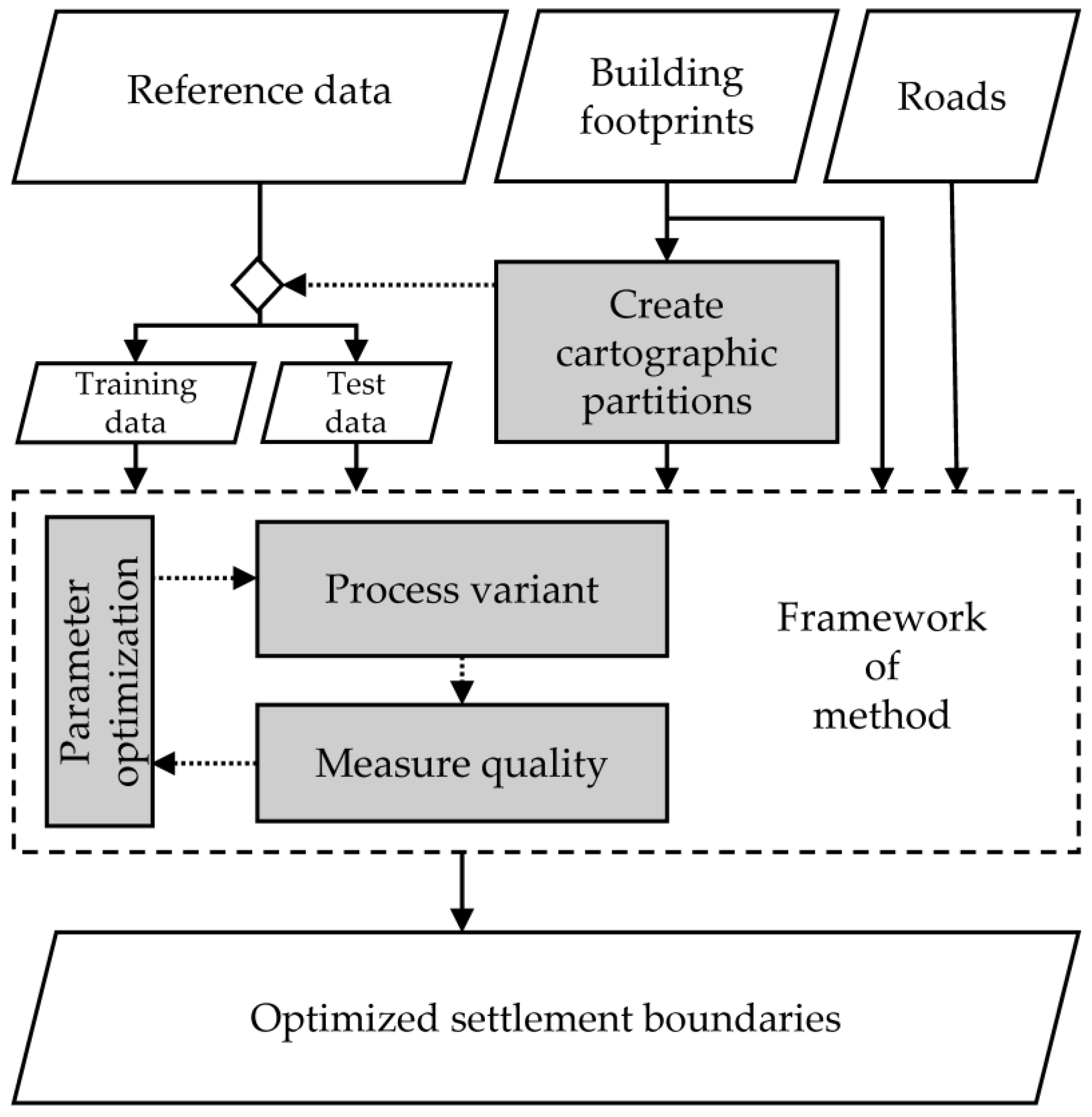
3.1. Workflow
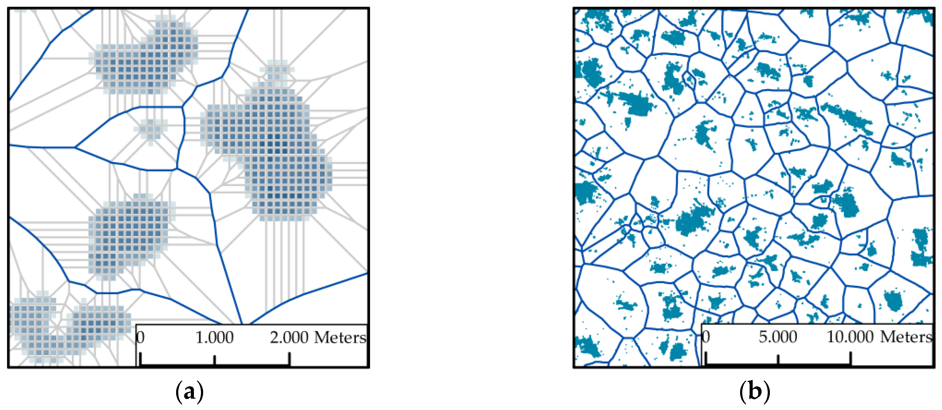
3.1.1. Create Cartographic Partitions
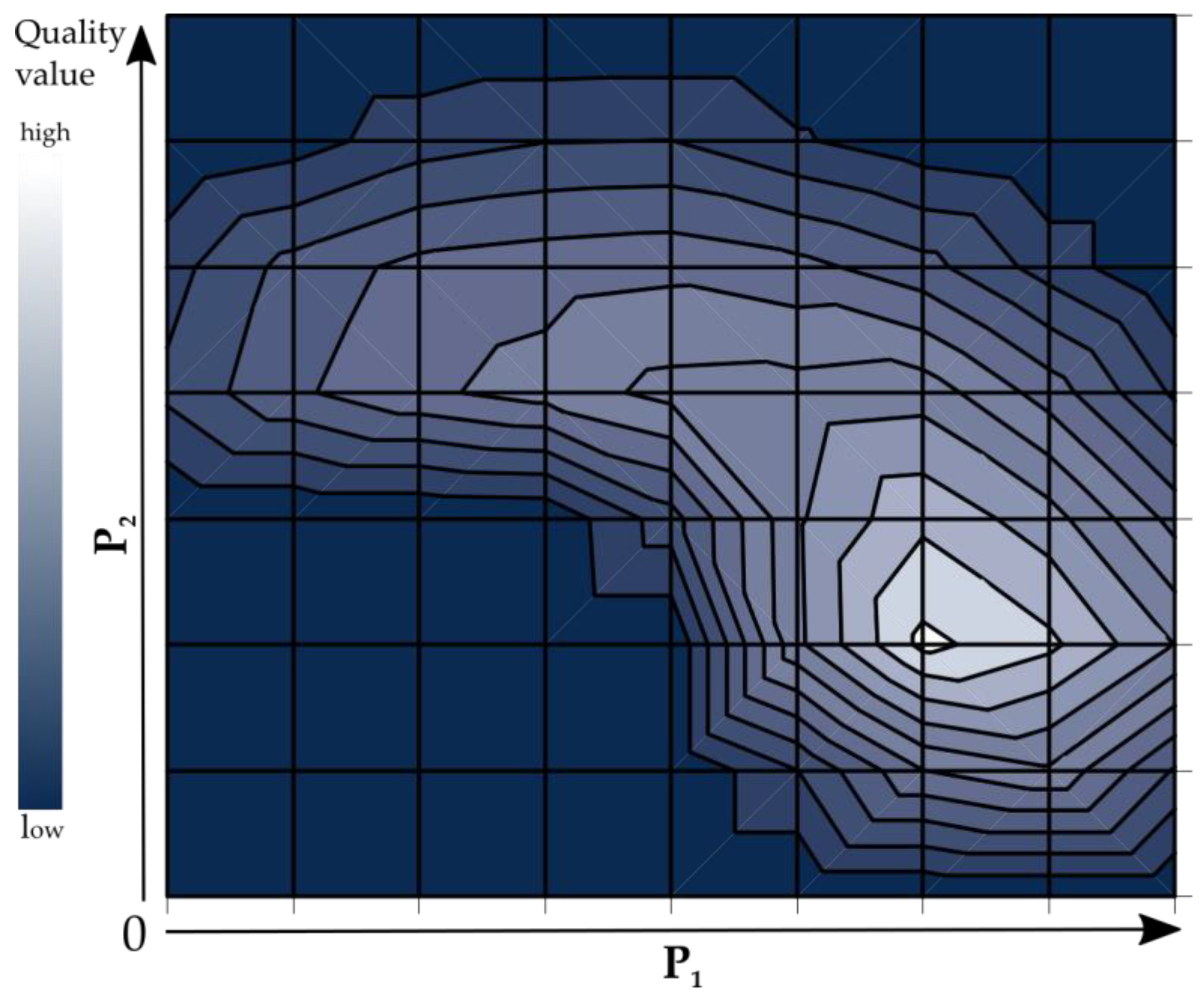
3.1.2. Parameter Optimization
3.1.3. Definition of a Geometric Quality Measure
3.2. Processing Variants
3.2.1. Delineate Built-Up Area Using Building Polygons (DBA-B)
3.2.2. Delineate Built-Up Area Using Building Polygons and Road Network (DBA-BR)
3.2.3. Delineate Built-Up Area Using Building Polygons and Road Network with Additional Pre- and Post-Processing (DBA-BRPP)
3.2.4. Delineate Built-Up Area Using Building Polygons and Road Network with Additional Pre- and Post-Processing and Urban Index (DBA-BRPPU)
4. Results
4.1. Data and Data Preparation
4.2. Comparison of Processing Variants
4.3. Precision and Recall
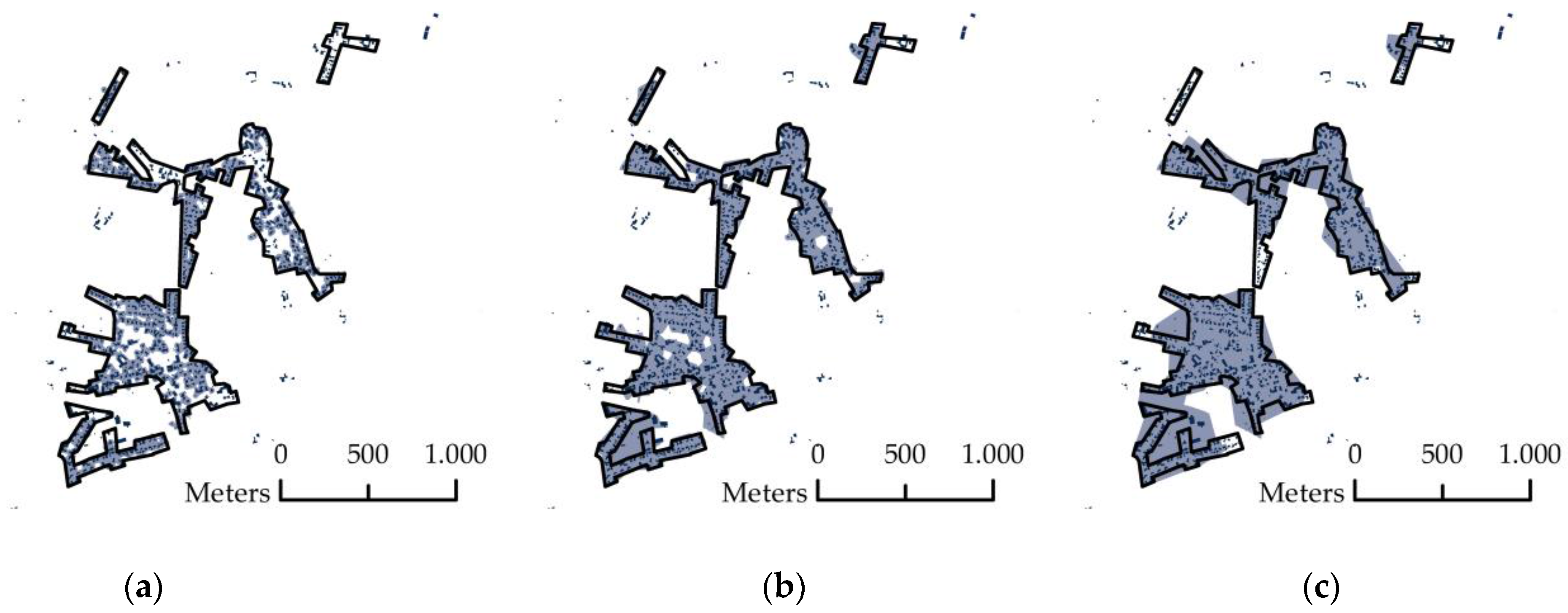
4.4. Visual Analysis of Variants
4.5. Types of Error
5. Discussion
5.1. Processing Variants
5.1.1. Variant DBA-B
5.1.2. Variant DBA-BR
5.1.3. Variant DBA-BRPP
5.1.4. Variant DBA-BRPPU
5.1.5. Comparison of Processing Variants
5.2. Discussion of the Approach as a Whole
5.3. Potential Applications
6. Conclusions
Acknowledgments
Author Contributions
Conflicts of Interest
References
- Jaeger, J.A.; Bertiller, R.; Schwick, C.; Cavens, D.; Kienast, F. Urban permeation of landscapes and sprawl per capita: New measures of urban sprawl. Ecol. Indic. 2010, 10, 427–441. [Google Scholar] [CrossRef]
- Siedentop, S.; Fina, S. Monitoring urban sprawl in Germany: Towards a GIS-based measurement and assessment approach. J. Land Use Sci. 2010, 5, 73–104. [Google Scholar] [CrossRef]
- Decoville, A.; Schneider, M. Can the 2050 zero land take objective of the EU be reliably monitored? A comparative study. J. Land Use Sci. 2016, 11, 331–349. [Google Scholar] [CrossRef]
- Zhou, Q. Comparative study of approaches to delineating built-up areas using road network data. Trans. GIS 2015, 19, 848–876. [Google Scholar] [CrossRef]
- Longley, P.A.; Mesev, V. On the measurement and generalisation of urban form. Environ. Plan. A 2000, 32, 473–488. [Google Scholar] [CrossRef]
- Mesev, V. Urban morphology reconstruction: links between satellite imagery and address information. In GIS and Evidence-Based Policy Making; Taylor & Francis: London, UK, 2010; pp. 9–42. [Google Scholar]
- Heikkila, E.J.; Shen, T.; Yang, K. Fuzzy urban sets: Theory and application to Desakota regions in China. Environ. Plan. B Plan. Des. 2003, 30, 239–254. [Google Scholar] [CrossRef]
- Zhou, Y.; Smith, S.J.; Elvidge, C.D.; Zhao, K.; Thomson, A.; Imhoff, M. A cluster-based method to map urban area from DMSP/OLS nightlights. Remote Sens. Environ. 2014, 147, 173–185. [Google Scholar] [CrossRef]
- Walter, V. Automatic Interpretation of Vector Databases with a Raster-Based Algorithm. Int. Arch. Photogramm. Remote Sens. Spat. Inf. Sci. 2008, 37(Part B2), 175–181. [Google Scholar]
- Hangouët, J.-F. Approche et Méthodes Pour L’automatisation de la Généralisation Cartographique; Application en Bord de Ville. Ph.D. Thesis, Université de Marne-La-Vallée, hamps-sur-Marne, France, 1998. [Google Scholar]
- Regnauld, N. Généralisation du Bâti: Structure Spatiale de Type Graphe et Représentation Cartographique. Ph.D. Thesis, Provence University, Marseille, France, 1998. [Google Scholar]
- Regnauld, N. Contextual building typification in automated map generalization. Algorithmica 2001, 30, 312–333. [Google Scholar] [CrossRef]
- Wertheimer, M. Untersuchungen zur Lehre von der Gestalt. II. Psychol. Res. 1923, 4, 301–350. [Google Scholar] [CrossRef]
- Boffet, A.; Serra, S.R. Identification of spatial structures within urban blocks for town characterization. In Proceedings of the 20th International Cartographic Conference, Beijing, China, 6–10 August 2001; pp. 1974–1983.
- Christophe, S.; Ruas, A. Detecting building alignments for generalisation purposes. In Advances in Geographic Information Science; Springer: Berlin, Germany, 2002; pp. 419–432. [Google Scholar]
- Yan, H.; Weibel, R.; Yang, B. A Multi-parameter approach to automated building grouping and generalization. Geoinformatica 2008, 12, 73–89. [Google Scholar] [CrossRef]
- Li, Z.; Yan, H.; Ai, T.; Chen, J. Automated building generalization based on urban morphology and gestalt theory. Int. J. Geogr. Inf. Sci. 2004, 18, 513–534. [Google Scholar] [CrossRef]
- Chaudhry, O.; Mackaness, W.A. automatic identification of urban settlement boundaries for multiple representation databases. Comput. Environ. Urban Syst. 2008, 32, 95–109. [Google Scholar] [CrossRef]
- Bundesregierung Perspectives for Germany: Our Strategy for Sustainable Development. Available online: https://www.nachhaltigkeitsrat.de/fileadmin/user_upload/English/pdf/Perspectives_for_Germany.pdf (accessed on 23 April 2016).
- European Commission. The Roadmap to a Resource Efficient Europe (COM (2011) 571). Available online: http://eur-lex.europa.eu/legal-content/EN/TXT/PDF/?uri=CELEX:52011DC0571&from=EN (accessed on 23 April 2016).
- Science for Environment Policy: No Net Land Take by 2050? Future Brief 14. Produced for the European Commission DG Environment by the Science Communication Unit, UWE, Bristol. Available online: http://ec.europa.eu/science-environment-policy (accessed on 3 August 2016).
- Battis, U.; Krautzberger, M.; Löhr, R.-P. Baugesetzbuch/BauGB; C.H. Beck: Munich, Germany, 2009. [Google Scholar]
- Brügelmann, H.; Dürr, H.; Bank, W.J.; Korbmacher, A. Baugesetzbuch/Kommentar; Kohlhammer: Stuttgart, Germany, 2011. [Google Scholar]
- Schiller, G.; Blum, A.; Hecht, R.; Meinel, G.; Oertel, H.; Ferber, U.; Petermann, E. Innenentwicklungspotenziale in Deutschland: Ergebnisse einer bundesweiten Umfrage und Möglichkeiten einer automatisierten Abschätzung; Bundesinstitut für Bau-, Stadt-und Raumforschung (BBSR) im Bundesamt für Bauwesen und Raumordnung (BBR): Bonn, Germany, 2013. [Google Scholar]
- Elgendy, H.; Michels, S. Raum+ Rheinland-Pfalz 2010: Die Bewertung von Flächenpotenzialen für eine zukunftsfähige Siedlungsentwicklung; Ministerium für Wirtschaft, Energie, Klimaschutz und Landesplanung: Mainz, Germany, 2011. [Google Scholar]
- AdV AdV Dokumentation zur Modellierung der Geoinformationen des amtlichen Vermessungswesens (GeoInfoDok)—Erläuterungen zu ALKIS®. Version 6.0.1; Arbeitsgemeinschaft der Vermessungsverwaltungen der Länder der Bundesrepublik Deutschland: Germany, 2008.
- Schiller, G.; Oertel, H.; Blum, A. Innenentwicklungspotenziale in Deutschland-Ergebnisse einer bundesweiten Befragung. In Flächennutzungsmonitoring V - Methodik, Analyseergebnisse, Flächenmanagement; Rhombos: Berlin, Germany, 2013; pp. 51–59. [Google Scholar]
- ArcGIS Resources Delineate Built-Up Areas. Available online: http://resources.arcgis.com/en/help/main/10.1/index.html#//007000000047000000 (accessed on 23 April 2016).
- Alpaydin, E. Introduction to Machine Learning; The MIT Press: Cambridge, MA, USA, 2010. [Google Scholar]
- ArcGIS Resources How Line Density Works. Available online: http://resources.arcgis.com/en/help/main/10.1/index.html#/How_Line_Density_works/009z00000012000000/ (accessed on 23 April 2016).
- Mackaness, W.A.; Ruas, A. Evaluation in Map Generalisation Process. In Generalisation of Geographic Information: Cartographic Modelling and Applications; Sarjakoski, L.T., Ruas, A., Mackaness, W., Eds.; Elsevier: Oxford, UK, 2007; pp. 89–112. [Google Scholar]
- Tveite, H.; Langaas, S. An accuracy assessment method for geographical line data sets based on buffering. Int. J. Geogr. Inf. Sci. 1999, 13, 27–47. [Google Scholar] [CrossRef]
- Vetter, A.; Wigley, M.; Käuferle, D.; Gartner, G. The automatic generalisation of building polygons with arcGIS standard tools based on the 1:50,000 Swiss National Map Series. In Proceedings of the 18th ICA Workshop on Generalisation and Multiple Representation, Rio de Janeiro, Brazil, 21 August 2015.
- Chaudhry, O.; Mackaness, W. Visualisation of settlements over large changes in scale. In Proceedings of the 9th ICA Workshop on Generalisation and Multiple Representation, La Coruña, Spain, 7–8 July 2005.
- Hecht, R.; Meinel, G.; Buchroithner, M.F. Automatic identification of building types based on topographic databases—A comparison of different data sources. Int. J. Cartogr. 2015. [Google Scholar] [CrossRef]
- Mas, J.-F.; Soares Filho, B.; Pontius, R.G.; Farfán Gutiérrez, M.; Rodrigues, H. A suite of tools for ROC analysis of spatial models. ISPRS Int. J. Geo Inf. 2013, 2, 869–887. [Google Scholar] [CrossRef]
- Bukies, K.; Meyer, H.; Rabe, E. Die Ermittlung der praktischen Grundlagen für die Festlegungen im Regionalen Raumordnungsprogramm 2005. In Steuerung der Eigenentwicklung in Ländlichen Siedlungen—Baustein Einer Nachhaltigen Flächenhaushaltspolitik; Beiträge zur regionalen Entwicklung; 123, Region Hannover: Hanover, Germany, 2009; pp. 29–43. [Google Scholar]
- Chesnokova, O.; Buffat, R.; Sieber, R.; Hurni, L. Depicting settlement development–extraction and visualization workflow. In Proceedings of the 27th International Cartographic Conference—16th General Assembly, Rio de Janeiro, Brazil, 23–28 August 2015.
- Provost, F.J.; Fawcett, T.; Kohavi, R. The case against accuracy estimation for comparing induction algorithms. In Proceedings of the ICML 5th International Conference on Machine Learning, San Francisco, CA, USA, 24–27 July 1998.
- Kotsiantis, S.B.; Zaharakis, I.; Pintelas, P. Supervised machine learning: A review of classification techniques. Informatica 2007, 31, 249–268. [Google Scholar]
- Hagedoorn, M.; Veltkamp, R.C. State of the art in shape matching. In Principles of Visual Information Retrieval; Advances in Pattern Recognition; Springer: Berlin, Germany, 2001; pp. 87–119. [Google Scholar]
- Mustière, S. Cartographic generalization of roads in a local and adaptive approach: A knowledge acquistion problem. Int. J. Geogr. Inf. Sci. 2005, 19, 937–955. [Google Scholar] [CrossRef]
- Steiniger, S.; Lange, T.; Burghardt, D.; Weibel, R. An Approach for the Classification of Urban Building Structures Based on Discriminant Analysis Techniques. Trans. GIS 2008, 12, 31–59. [Google Scholar] [CrossRef]
- Meinel, G.; Hecht, R.; Herold, H. Analyzing building stock using topographic maps and GIS. Build. Res. Inf. 2009, 37, 468–482. [Google Scholar] [CrossRef]
- Bovet, J. Handelbare Flächenausweisungsrechte als Steuerungsinstrument zur Reduzierung der Flächeninanspruchnahme. Nat. Recht 2006, 28, 473–479. [Google Scholar] [CrossRef]
- Henger, R.; Bizer, K. Tradable planning permits for land-use control in Germany. Land Use Policy 2010, 27, 843–852. [Google Scholar] [CrossRef]
- Schmidt, T. Innenentwicklungsbereich und Zertifikatpflicht; Flächenhandel—Informationspapier Nr. 3; Büro für Standortplanung Hamburg: Hamburg, Germany, 2014. [Google Scholar]
- Herold, H. An Evolutionary Approach to Adaptive Image Analysis for Retrieving and Long-Term Monitoring Historical Land Use from Spatiotemporally Heterogeneous Map Sources. Ph.D. Thesis, Dresden University of Technology, Dresden, Germany, 2015. [Google Scholar]
- Muhs, S.; Herold, H.; Meinel, G.; Burghardt, D.; Kretschmer, O. Automatic delineation of built-up area at urban block level from topographic maps. Comput. Environ. Urban Syst. 2016, 58, 71–84. [Google Scholar] [CrossRef]


| Parameter | Explanation |
|---|---|
| Input polygons | As input polygons we use building footprints. Their density and arrangement are used to define appropriate built-up polygons as output. |
| Output polygons | The output contains polygons of built-up area representing clusters of input buildings. |
| Grouping Distance (GRP) | Buildings that are closer together than the grouping distance are grouped together. The grouping distance is measured from the edges of building polygons to the center points of the buildings. |
| Minimum Detail Size (DET) | This value defines the relative degree of detail in the output polygons. This roughly corresponds to the minimum allowable diameter of a cavity in the output polygon. The actual size and shape of cavities within the polygon is determined also by the arrangement of the input buildings, the grouping distance, and the presence of auxiliary features, if they are applied. |
| Auxiliary data | This layer is used to define the edges of the output polygons. These snap to an auxiliary feature if it is generally aligned with the trend of the polygon edge and lies within the grouping distance. |
| Minimum building count (MCB) | This is the minimum number of buildings that have to be present to create an output polygon. |
| Topicality | Distribution Agency | Objects | Reference Scale | |
|---|---|---|---|---|
| ATKIS®—Ortslage | 2011 | NMAs 1 | 197 | 1:25,000 |
| ATKIS®—Roads | 2011 | NMAs 1 | 32.788 | 1:10,000 |
| Reference polygons | 2005 | Kommunalverband Region Hannover | 166 | 1:1000 to 1:2000 |
| Official Building Polygons (HU-DE) | 2011 | ZSHH 2 | 92.080 | 1:1000 |
| Para. DET/GRP | Ø (QBOM) | M (QBOM) | R | Max (QBOM) | Min (QBOM) | σ (QBOM) | |
|---|---|---|---|---|---|---|---|
| ATKIS®-Ortslage | - | 0.615 | 0.617 | 0.560 | 0.885 | 0.325 | 0.114 |
| DBA-B | 5/45 | 0.620 | 0.626 | 0.416 | 0.817 | 0.401 | 0.069 |
| DBA-BR | 5/45 | 0.679 | 0.690 | 0.367 | 0.811 | 0.444 | 0.069 |
| DBA-BRPP | 5/25 | 0.710 | 0.714 | 0.417 | 0.856 | 0.439 | 0.068 |
| DBA-BRPPU | 5/25 | 0.705 | 0.717 | 0.465 | 0.850 | 0.385 | 0.077 |
| DPA-B | DPA-BR | DBA-BRPP | DBA-BRPPU | |
|---|---|---|---|---|
| ATKIS®-Ortslage | 0.650 1 | 0.000 1 | 0.000 1 | 0.000 1 |
| DBA-B | 0.000 2 | 0.000 2 | 0.000 2 | |
| DBA-BR | 0.000 2 | 0.002 2 | ||
| DBA-BRPP | 0.567 2 |
| NTP | NFN | NFP | Precision | Recall | |
|---|---|---|---|---|---|
| ATKIS®-Ortslage | 164 | 2 | 17 | 0.91 | 0.99 |
| DBA-B | 165 | 1 | 48 | 0.77 | 0.99 |
| DBA-BR | 165 | 1 | 47 | 0.78 | 0.99 |
| DBA-BRPP | 161 | 5 | 7 | 0.96 | 0.97 |
| DBA-BRPPU | 160 | 6 | 5 | 0.97 | 0.96 |
| Area Ref. | Area Deli. | Area (TP) | Area (FN) | Area (FP) | Precision | Recall | |
|---|---|---|---|---|---|---|---|
| ATKIS®-Ortslage | 4683 | 5973 | 4403 | 141 | 1.429 | 0.75 | 0.97 |
| DBA-B | 4683 | 4016 | 2735 | 975 | 307 | 0.90 | 0.74 |
| DBA-BR | 4683 | 4468 | 3417 | 634 | 417 | 0.89 | 0.84 |
| DBA-BRPP | 4683 | 4690 | 3823 | 430 | 437 | 0.90 | 0.90 |
| DBA-BRPPU | 4683 | 4569 | 3682 | 501 | 386 | 0.91 | 0.88 |
| Frequency | Weighting | |||
|---|---|---|---|---|
| Systemic errors: | ||||
| False-negative classification | ||||
| Gaps in the boundary | high | medium | ||
| Empty spaces within the boundary | low | medium | ||
| Delineation not simplified on the edge | medium | low | ||
| Line-like settlement structures not delineated | medium | high | ||
| False-positive classification | ||||
| Areas included that formal do not belong to inner zone | medium | medium | ||
| Missing empty spaces within the settlement boundary | low | high | ||
| Data-induced errors: | ||||
| Adaptability of the periods of the data used | low | high | ||
| Parts of the settlement not includes in the reference | low | high | ||
| Buildings and areas included in the reference that formal do not belong to inner zone | low | high | ||
© 2016 by the authors; licensee MDPI, Basel, Switzerland. This article is an open access article distributed under the terms and conditions of the Creative Commons Attribution (CC-BY) license (http://creativecommons.org/licenses/by/4.0/).
Share and Cite
Harig, O.; Burghardt, D.; Hecht, R. A Supervised Approach to Delineate Built-Up Areas for Monitoring and Analysis of Settlements. ISPRS Int. J. Geo-Inf. 2016, 5, 137. https://0-doi-org.brum.beds.ac.uk/10.3390/ijgi5080137
Harig O, Burghardt D, Hecht R. A Supervised Approach to Delineate Built-Up Areas for Monitoring and Analysis of Settlements. ISPRS International Journal of Geo-Information. 2016; 5(8):137. https://0-doi-org.brum.beds.ac.uk/10.3390/ijgi5080137
Chicago/Turabian StyleHarig, Oliver, Dirk Burghardt, and Robert Hecht. 2016. "A Supervised Approach to Delineate Built-Up Areas for Monitoring and Analysis of Settlements" ISPRS International Journal of Geo-Information 5, no. 8: 137. https://0-doi-org.brum.beds.ac.uk/10.3390/ijgi5080137