1. Introduction
Georeferenced data is indispensable in different fields of the society while taking account of the need for data protection and the demand for high-resolution data (cf. [
1,
2]). With respect to large georeferenced datasets on buildings, the question arises: Which forms of data processing and analysis are best suited to establish new insights into the residential as well as the non-residential building sector? Whilst considerable data is gathered on the residential building stock, many European countries possess insufficient databases on the total stock of non-residential buildings. In addition to the numbers of buildings and footprint areas, researchers of different domains require robust data on the age and use of buildings, the ownership structures, the building quality and condition as well as related dynamic characteristics [
3,
4,
5,
6,
7,
8,
9]. Furthermore, building stocks have become the focus of political debate in light of challenges of resource efficiency, the impact of climate change, the rising danger of natural hazards and attempts to reduce CO
2 emissions. In order to ensure that decisions on the building stock are empirically-based, specific data on the total stock as well as information on the spatial distribution of selected building attributes is required.
In this respect, the objective of this article is to present a new methodological approach for data integration that considers commonly available geospatial data products and create a novel database. The processed data allows characterizing the structure and dynamic of national building stocks to a high level of detail. In particular, it allows the quantification of the total stock of residential and non-residential buildings. Thus, it supports future studies on the building stock as well as monitoring systems and political decision-making processes over the long term.
The article is structured as follows.
Section 2 provides a brief review of related work to quantify the total building stock and its spatial distribution.
Section 3 gives an overview of official building data products with the focus on Germany. In
Section 4, the case study area and used data sets are presented. The workflow, broken down to its constituent steps, is given in
Section 5, followed by exemplary results in
Section 6. Finally,
Section 7 and
Section 8 provide a discussion and summary of the presented workflow while some areas for future research are identified.
2. Related Work
Exhaustive statistical surveys are often supplemented by rough model estimates in order to quantify the national stock of buildings as well as changes to this. The large range of available geo- and remote-sensing data is used rather infrequently, and then only for analysis at the urban or regional levels. In the following, we discuss previous attempts at data gathering as well as various approaches to the semantic enrichment of geodata for more detailed monitoring of the building stock.
2.1. Previous Approaches to Quantify Building Stocks
In the past, various approaches have been attempted to try to quantify the national building stock (number of buildings and total built-up area) [
3,
9,
10,
11,
12,
13]. This can be attributed to the fact that most countries still do not conduct an exhaustive survey of buildings ([
14,
15,
16]). By summing the annual net increase in stock, it is possible to reconstruct the national building stock relatively well. However, without knowledge of the absolute size of the stock, such cumulative processes are unable deliver reliable figures for the total stock (e.g., [
17]). On the basis of a range of indicators for the building sector (e.g., average office space or production space per employee as well as usable floor space per hospital bed or per pupil/student), basic parameters of the total stock of buildings can be quantified using an indicator-based approach. However, such indicators are complex to research and are spatially so heterogeneous that only rather imprecise estimates can be made. The use of highly simplified extrapolation methods (e.g., to determine asset values, relations to the housing stock) can only produce some initial rough estimates [
18]. Using difficult-to-compile reference data, an attempt has also been made to determine previously unknown building stocks at the regional/local level [
1,
11,
12,
13]. In this context, multivariate statistical procedures have also been used in some cases to uncover significant interdependencies between stocks and other forms of data (construction of model equations, cf. [
19]).
In general, we can state that the named approaches in various countries only serve to produce indirect estimates of the total stock of buildings. It is normally impossible to validate the figures thus obtained as no reference data is available for comparison. On the other hand, geodata offers a new and promising approach to estimate total stocks as well as to classify buildings into sub-classes. Vector databanks of the National Mapping and Cadastral Agencies (NMCAs) supply information on addresses, footprints as well as details of usage for every building. The geometries are determined by on-site inspection or evaluation of aerial or satellite imagery. Some countries also maintain a tax register that enables a further description of buildings in regard to used floor area [
20,
21].
Today’s earth observation systems open up new potentials for gathering information and data on the building stock. Photogrammetric and remote-sensing methods allow the reconstruction of 2D and 3D object geometries by processing satellite imagery from such services as Ikonos, Quickbird, GEOEye-1 or WorldView-2 (e.g., [
22,
23,
24,
25]). An overview of image-based building extraction from aerial and satellite images can be found in [
26,
27,
28,
29]. However, such image data alone is usually insufficient for the consistent reconstruction of buildings as the detection rate of such remote-sensing approaches is often less than 90% (e.g., [
22,
30]). A fully automated, efficient and precise detection of buildings has only been possible since the development of airborne lasers canning (ALS). By combining images and LiDAR data, the detection rate can be increased to over 90% [
31,
32,
33]. However, at the moment, building related LiDAR data is only available for major cities and in most countries there are no such data sets at all. Of course, building usage cannot be directly distinguished using such remote-sensing techniques. In addition to the geometry, structural features such as the building size, height, shape as well as the type of roof can be determined. This information can then be used to specify the likely form of use (see next section).
2.2. Semantic Enrichment of Building Footprints
Data on building footprints give information on the number of buildings but is unable to directly assist in the classification of building type (e.g., usage classes, age classes, etc.). Therefore, in the past few years, methods have been developed to automatically classify buildings by analyzing building features derived from remote-sensing images and topographic data. According to their basic orientation, such methods can be divided into knowledge-based (“top-down”) and data-driven (“bottom-up”) approaches (cf. [
34]). Data-driven approaches make use of processes of machine learning to automatically train a classifier on a training data sample. Such training methods include unsupervised clustering approaches such as the expectation-maximization algorithm [
35,
36,
37] or supervised classification processes of pattern recognition and machine learning (e.g., [
34,
38,
39,
40]). While data-driven approaches are gaining in popularity, previous efforts have been experimental in nature and merely applied at the urban level. One challenge still to be overcome is the limited transferability due to regional factors (cf. [
34,
38]).
In knowledge-based approaches, buildings are classified to specific types by means of a rule-based system developed by an expert in a modeling process often through trial and error. The knowledge is often represented in the form of a hierarchical decision-tree or network that can be comprehended both by specialists and by computers. One set of rules is, for example, those applied by [
41] to classify buildings into six classes (middle house in a row, end house in a row, free-standing house, two-under-a-roof, apartment und special) by considering the Dutch real-estate cadaster, address coordinates and building plots. Also in the study by [
42], building footprints (OS MasterMap
®) are correlated with addresses to specify one of five classes (detached, semi-detached, terrace, flat, unclassified). A similar approach that also uses the OS MasterMap
® is described in [
43]. Here, six different types of residential building (detached, semi-detached, terraced, maisonette, flats indiv, flats contig) are identified for greater London. In the context of map generalization, Rainsford et al. [
44] developed a process based on template matching in which nine building forms are distinguished, using Latin lettering as orientation. Further ontological approaches for the semantic enrichment of digital topographic databases have been proposed by [
45,
46]. In the latter, ontological modeling is combined with a Bayesian inference model, i.e., knowledge-based and data-driven approaches. Alongside cadastral data, rule-based building classification approaches have also been applied to Digital Topographic Maps at a scale of 1:25 k [
47], remote-sensing data [
48] or Volunteered Geographic Information, such as from the OpenStreetMap platform [
49].
3. Building Definition and Representation in Geotopographic Databases
There are various approaches to the mapping of buildings in geospatial data. In the following we define the concept of a building before going on to discuss the representation of buildings in geotopographic databases from National Mapping and Cadastral Agencies (NMCAs). Finally, German Official Authoritative Geodata Products are introduced in detail, as they serve as a testbed for the development of the workflow.
3.1. Building Definition
Buildings are variously defined according to the chosen discipline and research perspective. For instance, the EU Directive on the energy performance of buildings provides the following definition as “a roofed construction having walls, for which energy is used to condition the indoor climate” [
50]. According to the Statistical Office of the European Commission (Eurostat), a building is a “roofed construction which: can be used separately; has been built for permanent purposes; can be entered by persons; is suitable or intended for protecting persons, animals or objects. Buildings do not necessarily need walls. It is sufficient for them to have a roof, but there must be a demarcation which constitutes the individual character of the building to be used separately...” [
51]. Individual buildings are either free standing or are separated from adjacent buildings by firewalls. At the very least, individual buildings should have a separate access system (entrance). This point is important as it allows us to correlate the building count in statistics and cadaster by assuming a correspondence between a building entrance and building coordinate. The Eurostat building definition cited above is similar to that used by the German Federal Bureau of Statistics (DESTATIS), the main difference being that Eurostat includes underground buildings and DESTATIS does not.
Buildings can be further classified as residential or non-residential. A building is regarded as residential if at least half of the useful floor area is used for dwelling purposes. Conversely, if more than half of the floor area is dedicated to non-residential purposes, the building is classified as non-residential [
51]. Residential buildings are further classified according to the number of dwellings and the living form (e.g., one-dwelling buildings, two- and more dwelling buildings and residences for communities). In addition, non-residential buildings are further subdivided into a range of types according to their form of usage such as hotels and similar buildings, office buildings, wholesale and retail trade buildings, traffic and communication buildings, industrial buildings and warehouses, public entertainment, education, hospital or institutional care buildings and other non-residential buildings [
51]. Of course, there exist alternative building typologies that make use of criteria such as the size and morphological form, building age or material [
7,
9,
52].
3.2. Building Representation in Digital Topographic Data
Buildings are represented in digital spatial data in various ways, for example as point data (address data), two-dimensional polygon data (real estate cadaster) or as a three-dimensional representation (3D city model). The most important data sources are digital topographic databases provided by the National Mapping and Cadastral Agencies (NMCAs). Building geometries are acquired in various ways. NMCAs usually capture the geometrical footprint of buildings by means of large-scale planimetric surveys involving field measurements and/or photogrammetric techniques. Nowadays, remote-sensing technologies, especially airborne laser scanning (LiDAR) and digital aerial imagery, enable a highly efficient reconstruction of the geometry. An additional source of historical data on buildings are digital or scanned topographic maps and plans.
Regarding 2D building footprints, two basic forms of representation can be distinguished in terms of semantics and geometry: The
single building representation and the
building region representation (
Figure 1). In remote sensing, for example, building footprints are extracted by image processing techniques (e.g., from LiDAR or aerial imagery). The geo-objects obtained in this way represent a single building or a group of adjacent buildings (
Figure 1b). This latter type of modeling is termed building region representation. Also in topographic maps, buildings are usually depicted in such representations as solid black areas with no detailed subdivision. In the digital cadastral databases of NMCAs, buildings are modeled in a single building representation. Each geo-object represents either a detached single building or a semidetached or terraced single building of a building complex.
In setting up a model to quantify building stocks, it is crucial to distinguish between these two forms of representation. In the presented case study, we refer to the address based building definition as this is the one used in statistical publications.
4. Case Study and Input Data
4.1. Study Area
The national territory of the Federal Republic of Germany covers more than 357,000 km
2 and is located between latitudes 47°N and 55°N and longitudes 5°E and 16°E. Germany’s system of governance operates at three levels: the Federal government (
Bund), the 16 federal states (
Länder) (see
Figure A1) and more than ten thousand municipalities (
Gemeinden). With a population of approx. 81 million, Germany is the most populous member state of the EU and has one of the world’s biggest economies measured by purchasing power parity. Both the population density and building density is generally higher in the western than in the eastern states, with the exception of Berlin [
1].
If we look at trends in the building sector over the last 25 years, construction measures within existing buildings have contributed a constantly increasing proportion of the volume of building work in most European regions. With an average annual value of 228.5 billion euro [
53], Germany’s construction sector is the biggest in Europe and serves to stabilize demand for the entire EU. In international comparison, Germany is recognized for its preeminent role in the field of stock maintaining measures [
54]. Against this background, the German building stock is used in the article as a reference example to illustrate the application of the developed workflow.
4.2. Input Data
NMCAs in Europe provide nationwide exhaustive spatial data on buildings with explicit modeling of single buildings. Requirements for modeling buildings in the EU are laid out by INSPIRE guidelines, whose building definition and classification is partly based on and adapted from the Eurostat classification of types of constructions [
55].
The most recent and most comprehensive German-wide data products are the “Official Building Polygons of Germany” (product name HU-DE) and address data as “Official House Coordinates of Germany” (product name HK-DE). These products follow standards on data formats and content set by the Working Committee of the Surveying Authorities of the Länder of the Federal Republic of Germany (AdV) and are distributed nationwide by the Zentrale Stelle für Hauskoordinaten und Hausumringe (ZSHH). For public authorities and science institutions, a slightly different version of this data is offered by the Federal Agency for Cartography and Geodesy (BKG). Alongside HU-DE and HK-DE, the agency offers a dataset of address coordinates called “Georeferenced Address Coordinates” (product name GA), which is an extended version of the HK-DE.
In the presented case study, we make use of the products HU-DE, GA and ATKIS, which are introduced below. To compensate for the fact that HU-DE does not contain any attributive information on building usage and due to the limited accessibility of nationwide cadastral data (e.g., Authoritative Real Estate Cadaster Information System (ALKIS)), land use data from the German Authoritative Topographic Cartographic Information System (ATKIS) is used as a substitute.
4.2.1. Official Building Polygons of Germany (HU-DE)
HU-DE is a
polygon dataset containing over 50 million geo-referenced footprints of buildings derived from the Authoritative Real Estate Cadaster Information System (ALKIS) of the federal surveying and mapping authorities of the German States. ALKIS is the official register of all land parcels and buildings in Germany, produced and continuously updated by regional cadaster authorities. According to the data format description, the HU are objects in the form of georeferenced polygons that describe geometrical building outlines. According to the product specification, these do not include any design geometries, roofs, or underground buildings and do not provide any attributive information on building usage, ownership or building age [
56]. The objects have only one attribute field, which is the official municipality key (AGS).
4.2.2. Georeferenced Address Data (GA)
The GA is a
point dataset defining the spatial position of all buildings across Germany with addresses. This data is an extended version of the data product HK-DE [
57] of official building coordinates by including third-party addresses from the German postal company
Deutsche Post direkt GmbH and by unifying administrative references (e.g., municipality key, street names, etc.). The main data source is the real estate cadaster ALKIS of the German States, which assigns an official house number to parcels and main buildings. Outbuildings may be assigned an (internal) pseudo-number. By means of field surveys, the official house number is georeferenced to the entrance of a building. In the case of planned and ongoing building projects, address coordinates may only be assigned to land parcels. A particular quality attribute describes the positional accuracy of the address (
Table 1). A visualization of both building related data sources is given in
Figure 2, an overview of data specifications is presented in
Table 2.
4.2.3. Land Use Data (ATKIS)
Building polygon or address point datasets do not provide information on buildings, which is instead taken from the ATKIS Basis-DLM. ATKIS is the most comprehensive object-structured model of land use and topography in Germany. In a narrower sense, ATKIS is a Digital Landscape Model (DLM) while also serving as a foundation for Digital Topographic Maps as well as Digital Terrain Models (DTM) and Digital Orthophotos (DOP). The abstract model of ATKIS describes the landscape exhaustively (i.e., without gaps) and without overlaps, using points, lines and polygons. Topographic lines such as streets, footpaths and rivers form a network whose meshes are filled by polygons of actual use. Land use information is modeled in object groups [
58]:
41000 Settlements
42000 Transport
43000 Vegetation
44000 Water
The principle of dominance is applied to define the usage type of a mesh, i.e., the area-wise dominant usage is assigned to the whole mesh. It is important to note that the building usage information assigned to these meshes is accompanied by a certain level of generalization. There are 14 object types used in this analysis, the following are mentioned as the most relevant types in the context of building usage as indicated by the encoding (examples are taken from the settlement object group):
Residential Use (AX_41001)—more than half of the mesh area used for housing
Mixed Use (AX_41006)—no dominant usage type within mesh
Industrial and Commercial Use (AX_41002)—more than half of the mesh area used for commerce or industry
Special Use (AX_41007)—more than half of the mesh area dedicated to special use (e.g., hospital, school)
5. Workflow
The workflow for an automatic quantification of structure and dynamic is depicted in
Figure 3. This encompasses several steps: (1) data pre-processing; (2) calculation of building attributes; (3) semantic enrichment; (4) intersection with spatial units; and finally (5) quantification of the building structure and dynamics based on the defined spatial units. The processing Steps (1) to (4) are performed for each time point whereas (5) uses the results for each processing point. As mentioned in
Section 4, no semantic information on building type (i.e., detached, semi-detached or row) is available for the building footprints. Using auxiliary data such as address data and the digital landscape model from ATKIS, a set of building attributes describing the characteristics of buildings is derived for a rule-based classification. All processing steps are implemented within a Toolbox in ArcGIS 10.3 (Advanced License) using Python (
www.python.org) scripts. This is explained in greater detail below.
5.1. Data Pre-Processing
The basis for a robust quantification of the building stock is a dataset with homogenous modeling of buildings and no overlaps or any other inconsistencies. Especially when data sets of various sources are combined, one has to expect some differences. It depends on the extent of these inconsistencies and their relevance, and how such issues are dealt with. Considering building stock analysis, the geo data should make it possible to quantify buildings in number and area. Therefore, it should be defined, with respect to data specification and eventual legal prescriptions, how buildings are represented and if there are possible size limits to sort out non-buildings. Visual and automatic inspection of the original data revealed errors in topology and semantics (overlaps, non-building polygons, atypical polygons). The general automatic approach to prepare the building polygons begins with a removal of overlaps, a process that can result in newly added polygons and non-building geometries. In consequence, it is followed by a threshold based removal of non-buildings. Summarizing, the found issues are eliminated with the following pre-processing steps:
- (a)
Resolving topological inconsistencies
- (b)
Removal of small polygons
- (c)
Removal of atypical polygons
5.1.1. Solving Topological Inconsistencies
A topologically consistent vector dataset should be free of any polygon overlaps as this can lead to an overestimation of the building stock in terms of number and areas. In order to analyze polygon contiguity, the ArcGIS tool PolgonNeighbors_analysis (PNA) is used to create a table of adjacent polygons pairs (source-polygon and neighbor-polygon) with statistics on their area of overlap. In relation to the areas
of the polygons involved, the overlapping area
can be used to characterize an overlap type as follows:
The identified topological inconsistencies are removed automatically in a two-step approach (see
Figure 4). Firstly, a union of all polygons is calculated, by which all intersection points between overlaying polygons are created as new nodes of the overlapping areas. In the resulting dataset, the overlapping areas are segmented into single polygons and overlay each other as duplicates. The IDs of these polygons are identified by a polygon neighbor analysis and half of these is selected for deletion. In the second step, the other half is selected and aggregated to the adjacent polygon with the longest shared border. Geometries are changed during overlap removal and it is possible that new polygons are created. Mostly this occurs when complex overlaps are removed. The following steps help to minimize any negative effects of these geometric changes.
5.1.2. Removal of Small Polygons
Some of the polygons in the dataset are too small to be buildings and may actually represent projecting roofs, tool sheds or balconies. Therefore, all polygons with an area smaller than 10 m
2 are identified as some non-building structure. The threshold of 10 m
2 has been derived from standardized building and surveying codes, e.g., [
59]. Polygons below that size are either classified as “non-building” if solitary or are aggregated to the adjacent polygon with the longest shared border.
5.1.3. Removal of Atypical Polygons
In this last step of pre-processing, atypical polygons are identified and removed from the data. Atypical polygons are characterized by a very slim and winding shape. The polygons are often adjacent to other polygons and a separate usage seems very unlikely when their area is below a certain size.
The identification is based on area
and perimeter
of the polygon and a defined measure of compacteness
using the Iso-Perimeter Quotient (IPQ) as the shape index [
60]:
This value is stored as attribute SHP_IDX and continually recalculated after geometric changes to the data set. Empirically determined thresholds for
and
serve as a basis for the identification of atypical polygons. Based on a rectangular geometry a
-value of 0.3 would imply a width/length-ratio of 1–8 (see examples in
Figure 5). This was taken as an unusual shape for a single building geometry. However, considering building regions or large buildings, these values can occur, so in addition an area threshold was necessary. By evaluating histograms of polygon areas for a given shape index, it was possible to determine a minimum polygon area that would allow for a distinction of groups in the population of atypical polygon shapes (see vertical line in
Figure 6).
Thus, polygons with a value of less than 0.3 and area below 190 m2 are considered as atypical buildings and are aggregated to their adjacent polygon with the longest shared border. In case of solitary polygons, these will remain in the data set but are flagged.
5.2. Building Attributes
In this process, the buildings are described by a set of building attributes as a basis for classification. Some attributes are derived by intersection with the address point data and land use data from ATKIS (e.g., number of addresses in polygon, land use type). Some building attributes are derived from the building polygon dataset itself (e.g., area, number of adjacent polygons, etc.).
5.2.1. Determination of the Land Use Type
First, the land use type is derived by spatially joining the building polygon data with the land use information from the ATKIS digital landscape model. For each building polygon, the land use code is obtained using the SpatialJoin_analysis tool with “HAVE_THEIR_CENTER_IN” as the relationship option. Since the ATKIS meshes are generated by the axis of linear topographic objects (e.g., street axis), it is very unlikely that there are ambiguous overlap situations between land use meshes and building polygons. However, the chosen join relationship should result in an unambiguous join. After this step, the building polygons carry the attribute OBJART with the codes of the ATKIS land use class.
5.2.2. Calculating the Number of Addresses
In the next step, the number of address points per building polygon is calculated. A tolerance is introduced in order to match the building polygon data with the address point data. Specifically, a buffer distance is set to 2 m using the SpatialJoin_analysis tool from ArcGIS with the “CONTAIN” and “WITHIN_A_DISTANCE” option. In order to reduce ambiguities, the buffer distance is set to a lower value than the distance space between building and parcel border as stipulated in the German Model Building Code [
61]. The buffer is only applied to the coordinates outside a building polygon, so in the process these outside coordinates are selected and matched in advance. Each of these join operations calculates a “Join_Count” attribute so that the sum of these counts is the number of addresses per building. The value is stored in the attribute ADDNUMB, which is useful for separating main buildings from outbuildings.
5.2.3. Calculating Topological Properties
For the identification of morphological types, i.e., detached, semi-detached or terraced, the number of adjacent polygons is calculated for each building region. In a first run, all neighbors of a polygon are considered (N_NBR), in a second run only neighbors among addressed buildings areare calculated (N_NBR_ADD). Again, this is done using the function PolygonNeighbor_Analysis and evaluating its result tables. The address count within a polygon and the number of its addressed neighbors determines the classification of morphological types and the counting of separate buildings (see
Section 3.1).
5.2.4. Calculating Geometric Properties
During pre-processing there are changes on feature geometries, so geometric properties like shape area and perimeter have to be updated afterwards. This is done automatically within the file geodatabase. After finishing all geometric processing the shape index (SHP_IDX) is updated.
Table 3 shows the relevant attribute set that is used in the decision tree of the classification.
5.3. Semantic Enrichment
After calculating attributes, the building footprint data is semantically enriched with building type information. In order to assign a class code to each polygon a pre-defined hierarchical rule set is applied,
Figure 7 shows the used building typology. Initially, all non-buildings are discarded before the buildings are further classified according to the underlying land use type (LUT). The information of the number of address points helps to distinguish the main building and the outbuilding on the next level. Finally, for residential and mixed used buildings, the morphologic type (detached, semi-detached and terraced) is distinguished by using the sum of ADDNUMB (number of matched addresses) and number of addressed neighbor polygons (N_NBR_ADD). In the classification process the attribute field CLASS is added to the building polygons and an alphanumeric string value (class code) is built. The format of the class code is “A0000”, where the leading character denotes the usage type of the class and the following positions provide information about building rank and morphologic type (the second and last position). Within an update cursor iteration on the features, the previously calculated fields are evaluated and CLASS values are determined. The construction of a class string is presented in this pseudocode:
| Algorithm 1 ClassCode |
| 1:if OBJART in ListOfATKISResidential: |
| 2: usage = “R” |
| 3:elif OBJART in ListOfATKISMixed: |
| 4: . #repeated check for ATKIS usage class |
| 5: . #(usages “R”esidential, “M”ixed, “I”ndustial, “S”pecial |
| 6: . #Function, “T”ransport, “O”ther) |
| 7:else: usage = “O” |
| 8: |
| 9: |
| 10:if ADDNUMB = 0: |
| 11: rank = “2” # outbuilding |
| 12:else: |
| 13: rank = “1” # main building |
| 14: |
| 15:if usage in [“M”, “W”] and rank = “1”: |
| 16: if ADDNUMB + N_NBR_ADD > 2: |
| 17: mtype = “3” # morphologic type for residential usage |
| 18: else: |
| 19: mtype = ADDNUMB + N_NBR_ADD |
| 20: |
| 21:else: |
| 22: if N_NBR = 0: |
| 23: mtype = 0 |
| 24: else: |
| 25: mtype = 1 |
| 26: |
| 27:classcode = usage + “0” + rank + mtype + “0” |
| 28: |
| 29:#Example: M0130 for mixed usage main building of terraced type |
| 30:# S0210 for undetached outbuilding of special function |
A last step of classifying the morphologic type is a correction for end-of-row polygons. Since they only have one addressed neighbor, they are recognized as semi-detached. Therefore, a layer of only terraced polygons is used to select eventually adjacent addressed polygons in the original layer by location. Finally, these polygons are reclassified as terraced and the classification process is finished.
For the subsequent quantification of the residential building stock, only the addressed buildings of residential and mixed use are considered.
5.4. Intersection with Spatial Units
After classification, the footprints are spatially intersected with spatial reference units as a basis for tabular quantification and visualization of results. This is done by a spatial join of the identifier keys of the respective spatial units to the footprints (join relationship “HAVE_THEIR CENTER_IN”) Initially, the footprints carry the municipality key AGS (a 8-digit number code), allowing the derivation of statistics at the administrative level. By subdividing the keys, it is possible to select at higher administrative levels such as counties and federal states. In recent years the number of counties and municipalities has fallen due to administrative reform. In the case study, we make use of data reflecting the most recent municipal structure from (in 2015 there were 11,116 municipalities in Germany).
Reflecting the possible variation over time of administrative units [
62] raster or grid areas are gaining popularity in statistical reporting. In several countries recent censuses have been aggregated based on raster grids (Austria, Sweden, The Netherlands). The most frequently used raster type is based on squares, although other geometric primitives (hexagons, triangles, etc.) are possible. In this study, the regular squared EEA reference grid of cell size 10 km has been used to assign cell codes of the grid to each building polygon (see
Figure 8).
Finally, spatial typologies of regions are used to specify spatial units. These typologies have been developed by the Federal Institute for Research on Building, Urban Affairs and Spatial Development (BBSR (
http://www.bbsr.bund.de)) and are a way to regionalize the country based on socio-geographic parameters. By analyzing population figures, it is possible to characterize urban-rural regions in terms of numbers of commuters, economic sectors and centrality of workplaces. With the aforementioned AGS keys, it is possible to link municipalities to a region type (e.g., rural region, region with tendency of urbanization, region with urban character) that is joined to the attribute table of the footprints. When used to aggregate municipalities by their region, the resulting delineation is slightly bigger than county level. Since the regionalization is based on variable parameters, the resulting delineations may change over time.
5.5. Building Stock Structure and Dynamic
In this step, the current building stock structure and the changes are calculated for each time point, differentiated according to each building type and the defined spatial units. For each polygon, the number of buildings is calculated. Generally, all polygons above the 10 m2 size threshold are considered as buildings so their building count is 1. In case of addressed buildings the building count is set to the address count (ADDNUMB). The number of buildings is obtained by adding up the building counts per polygon. Stock changes have to be calculated within a fixed statistical reference area, so either uniform administrative or time-stable reference areas. Raster maps are used to visualize the spatial distribution of the changes.
6. Results
The presented workflow was applied to the building polygons and address data of the years 2011–2014. Given the scope of the data and the variety of possible ways to examine and analyze them, the presented results can only depict an extract. The results are presented in close relation to the procedural steps of the workflow. Raw data statistics and preprocessing statistics are highlighted. Structural and dynamic characteristics of the German building stock are demonstrated on different spatial scales. Changes are presented for the timeframe 2012–2014 and the results are furthermore compared to some official buildings statistics [
63].
6.1. Raw Data Statistics
The first inspection of raw data leads to some basic statistics regarding the total number of objects and corresponding building footprint areas as well as the number of georeferenced objects over time (cf.
Table 4). In the year 2014, there are about 51 million building polygons and about 22 million georeferenced objects. The total sum of footprint area accounts for 5765.1 km
2 and the mean footprint size is approximately 112 m
2. When looking to the annual development an increase of object numbers is obvious in all inspected data products. The average increase of building polygons is 898.358 features per year, compared to an average annual growth of 112.004 address coordinates.
Figure 9 gives a first impression of the amount of georeferenced addresses (GA) per federal state. A large amount of objects can be found in North Rhine Wesphalia, Bavaria, and Baden Württemberg. The federal city states are obviously characterized by the lowest numbers. Concerning the quality attributes of the georeferenced addresses, 95% of the official coordinates (quality T is omitted from analysis) are of quality A (coordinate inside building footprint). There is a certain variability in the occurrence of qualities B (coordinate inside parcel) and R (coordinate inside parcel without a corresponding building).
6.2. Preprocessing Statistics
Data pre-processing identifies and resolves topological inconsistencies, small polygons and atypical polygons.
Figure 10 shows the topological inconsistencies in the raw data of the year 2014 per federal state. According to the typology of overlaps, an evaluation showed that sliver and complex are the most common overlap types. For example, Baden-Württemberg (BW) and Bremen (HB) show a high portion of sliver overlaps. These overlaps are often associated with complex buildings of industrial, commercial or administrative function. Such overlaps are seldom found among residential buildings.
Table 5 shows the amount of identified small and atypical polygons which are removed in the preprocessing step. It can be stated that there are considerable inhomogeneities in the way the building footprints are modeled in the federal states of Germany. For example, in the state of Hesse (HE) 17% of the 4.9 mio. raw data polygons have an area of less than 10 m
2. Compared to the other states, HE shows a very detailed modeling of building parts.
The number of polygons of atypical shape is significantly lower than the number of small polygons. In summary, the share of atypical polygons is not higher than 1% in all federal states. The whole pre-processing leads to a reduction of the total number of polygons 6.5% (from 51,072,807 to 47,741,365).
6.3. Structure
According to the presented hierarchical classification scheme (cf.
Figure 7), it is possible to characterize the structure of the German building stock. Land use classes, main and out buildings as well as morphological characteristics can be derived. The class counts are presented in
Table 6. The buildings classified as residential or mixed use sum up to more than 90% of the stock. It should be mentioned that the land use class is just an indicator for the building usage. Profound building functions are not available at the moment for entire Germany. Against this background, thematic uncertainties are obvious. For example, 30.2% of the total building stock are outbuildings localized on a residential land use class. This class is dominated by garages, sheds and small annexes.
Figure 11 shows the amount of buildings and the proportion of main and out buildings per federal state. Main buildings and outbuildings are classified whether they are addressed or not. North Rhine-Westphalia shows the largest building stock (approximately 9.5 m. buildings: 4 m. main and 5.5 m. outbuildings). In most states, less than half of the footprints can be categorized as main buildings, higher portions only occur in the city states Berlin (BE), Hamburg (HH) and Bremen (HB).
Several characteristics of the German building stock are additionally visualized on the level of NUTS-2-Regions in
Figure 12.
Figure 12a shows the building density (all buildings considered) and the amount of main and out buildings. A disparity between East and West Germany is obvious concerning the density of buildings. When looking to the regions with a higher building density, the amount of main buildings is higher. In contrast, the rural regions are characterized by many outbuildings.
Figure 12b shows also the density of buildings and the proportion of residential and non-residential buildings (cf.
Figure 8). It reflects the aforementioned difference between urban and rural regions, which have a higher portion of residential buildings. Regions with the highest building density are for example: DEA1 (Düsseldorf), DEA2 (Cologne) as well as DE71 (Darmstadt including Frankfurt Main).
Figure 12c shows the density of residential buildings and the proportion of morphological buildings types.
As expected regions with high density have a lower portion of detached buildings and a higher portion of terraced buildings. Overall, 62% of the buildings in the residential class are counted as detached, 18% as semi-detached and 20% as terraced.
6.4. Dynamics
6.4.1. Dynamics of Usage Classes
The change of main buildings is also visualized on the level of NUTS-2-Regions in
Figure 12d. The highest change of main buildings is localized in typical urban regions such as Rhein-Ruhr, Rhein-Main, Munich, Berlin and Hamburg. A constant or slightly negative development is often found in the border regions or in typical peripheral regions such as the High Black Forest. The analysis of geodata offers also the possibility to identify outliers. These outliers need further investigations on the local level to decide about demolished or newly constructed buildings.
Table 7 shows the absolute change of building counts of residential (including mixed usage) and industrial main buildings from 2012 to 2014. The growth rate of industrial and commercial buildings is much higher than in the residential stock. Further investigations are necessary to get a deeper understanding of unusual values (e.g., growth rate of residential main buildings in MV or growth rate of industrial and commercial buildings in HB and HH). In addition to the federal building statistics the results of the workflow form a good basis for further discussions of unusual or surprising values.
6.4.2. Dynamics of Morphologic Types
A more detailed view on the morphologic types in the aforementioned residential building stock is presented in
Table 8. Here, the stock difference from 2012 to 2014 is broken down to the percentage contribution to the increase for each morphologic type. Generally, the classes of detached buildings contribute the biggest part to the stock change. The relatively high portion of detached buildings in the stock increase in Brandenburg (BB) can be attributed to the region around Berlin. The urban fringe of the capital is a region with growing population and a high construction activity.
6.5. Comparison with Official Statistics
For the residential building stock of the year 2014, the comparison with the official statistics [
63] (based on the census 2011) is given in
Table 9. In most states, the stock count derived from geodata is higher than the official count, with the highest discrepancy between both occurring in the state of Brandenburg (BB). In total, the count of the residential building stock derived from the geodata is ca. 5% higher than the stock of official statistics.
7. Discussion
The presented workflow allows, for the first time, an automatic quantification of the German national building stock in terms of structure and dynamics by using topographic spatial vector data from NMCAs. The following aspects will be discussed concerning a couple of methodological challenges and the used data: practicability/transferability, limited validation ability, limitations to quantify building structure and dynamic, input data quality aspects.
7.1. Practicability/Transferability
The proposed workflow has been developed, tested and demonstrated for the whole country of Germany. When designing the workflow, special care has been taken that only common geospatial data on buildings, land use and addresses are used. This data is considered in the Infrastructure for Spatial Information in the European Community (INSPIRE) themes and data specifications in Europe and secures the applicability to other European countries. However, the approach can also be applied to other countries outside of Europe where comparable data of appropriate quality is available. This may require some adaptations to the respective data model (e.g., land use codes) or revision of some model parameters.
7.2. Limited Validation Ability
A big challenge is the limited ability to validate the proposed workflow as a whole due to the lack of real ground-truth observations. The approach sets up on authoritative spatial data which are often considered to be the reference itself. We decided to assess the approach by comparing the numbers of the residential building stock with official statistical data. The comparison shows small differences and plausible patterns when looking at the building structure. With regard to the non-residential buildings, there is no official statistical data available for a comparison. At this point, one can only trust to the official geodata and the specified accuracies provided by the NMCAs. However, future research may focus on a profound accuracy assessment which should be supported by a comparison with digital orthophotos. To achieve this, the standard data quality parameters (e.g., completeness, logical consistency, thematic accuracy, positional accuracy) of the ISO 19157: 2013 [
64] should be considered. Due to the large extent of the area under investigation (in our case nation-wide) and the concurrent large number of buildings, only a systematic approach based on representative samples is feasible.
7.3. Limits to Quantification of Building Structure
The approach for the quantification the building structure considers different building characteristics such as the underlying land use type, building rank and the morphological type. A hierarchical rule set has been developed to classify the buildings into a set of predefined classes. This knowledge-based approach provides already rough national figures on the structure of the building stock, but further model enhancements might be feasible for a more detailed differentiation of the buildings (e.g., apartment building, single family homes). In this context, a more comprehensive set of attributes, which takes proximity of buildings into account, has to be calculated and evaluated, and data-driven approaches for building classification may be considered that make use of modern pattern recognition and machine learning techniques (e.g., [
34,
38,
46,
65]). In addition, new data products will be available in future containing information of building height and roof type with full coverage (e.g., 3D building model of Germany). The improved data products and the consideration of new methods can lead to even more detailed description of the building structure.
Furthermore, the approach is based on parameters which are derived from regulations or are empirically determined. In particular, the choice of threshold values for the removal of small and atypical polygons in the pre-processing (e.g., shape index, size) have an impact on the total stock. For example, a threshold of 10 m2 was set as a minimum size for objects to be considered as buildings. The threshold was derived from Building Codes and legal regulations on how a building is defined in statistics and surveying. The influence of the threshold values on the stock quantities, however, should be addressed in future studies.
Another model assumption is that only addressed buildings can be main buildings. For residential buildings, this assumption seems valid because every house resident usually has a postal address. Exceptions are a few residential rear houses that may do not have a separate address. For non-residential buildings the separation of main buildings and outbuildings based on addresses seems at the moment rather vague. A large number of non-residential buildings without an address may still have the character of a main building with own infrastructure provision, but only postally relevant buildings (e.g., of an industrial complex) are. This should be considered when interpreting the quantities of non-residential buildings.
7.4. Limits to the Quantification of Building Dynamic
Looking at the results of the dynamics, large differences between the federal states are observed. For example the changes of the residential building stock ranges regionally from 0.7% to 4.7%. Further research is needed to better understand the causes and effects of the changes. In this context, one should also note that the building stock is subject to continuous changes caused by new construction, refurbishment, renovation, conversation or demolition. In the approach presented here, the dynamics are represented only by changes in the total sums at the level of the chosen reference areas. This simplified view provides at the moment no quantities of new constructions or demolitions. Therefore, the approach should be improved by the introduction of a mechanism that allows a change detection on the level of individual buildings. However, one of the big challenges is the automatic assignment of homologous buildings at different time points. Due to possible changes of the geometric representation of buildings, suitable polygon matching algorithms need to be implemented for an unambiguous assignment [
66].
Another challenge of quantifying building stock dynamics is the choice of a reasonable monitoring (time) interval. In most German federal states there is a legal obligation of the owner to register construction measures of buildings or changes to buildings of certain extend and have them surveyed. But it takes between one to two years from the building construction to the survey of the building to the recording in the real estate cadaster database and to the appearance in the official German building polygon dataset (see also [
67]). While this system works in most states, the state of Thuringia changed the cadaster update management and solely uses aerial stereo imagery to update buildings to the cadaster. With an update cycle of two years, this system is currently in a test phase and it is not unlikely that other states will implement it as well. Considering input data actuality, the data set with the longest update cycle is the ATKIS data set, with up to five years for some features. Therefore, we suggest a rather conservative interval for monitoring the building stock development of 5 years or if yearly data is available by calculating 5-year mean values and deriving the yearly differences.
7.5. Input Data Quality Aspects
The accuracy of any model is heavily dependent on the quality of the used input data. The proposed approach sets up on relatively new secondary data products (building polygons and address data). According to the data providers the data may still contain some errors and inconsistencies. Visual inspection using digital aerial imagery revealed some data quality issues which can be different in the German states and the different time points. For example, we identified small polygons such as winter gardens, balconies, underground buildings, etc. According to the model description of the building polygon dataset, these polygons should not be counted as individual buildings and not be included in the database. Most objects can be identified and removed automatically in the pre-processing. However, some individual polygons remain undetected. Currently, this error cannot be quantified by the lack of suitable reference data. Furthermore, it was found that some buildings are entirely absent in the federal states Saxony and Mecklenburg-Vorpommern. This fact could be confirmed by the local surveying agencies responsible for the real estate cadaster. Further missing building polygons can occur especially in regions with current construction activities. An indicator to estimate number of new constructed buildings is the share of georeferenced addresses of quality “B” (c.f.
Table 1). In 2014 the portion of these coordinates was approx. 0.68% for the entire data set, which is in fact a relatively small amount of buildings.
It has to be mentioned, that German cadastral mapping agencies are subject of a process of change related to migration processes from the former German ALK data model to the new ALKIS-data model [
67]. This may lead to changes in the cadastral data but it is very likely that the data quality continues to improve in the future. The often used VGI data from the OpenStreetMap (OSM) project are currently unsuitable. Previous studies show that completeness of the building footprints is currently still too low, especially in rural areas [
68]. On the other hand, Fan et al. [
69] noted a not insignificant amount of newly constructed buildings in OSM which are not yet recorded in official data sets. Therefore, it remains for future research to explore how OSM data can be used in models for the quantification of building stocks as supplementary data.
8. Conclusions
A new workflow for the quantification of building stocks is proposed that uses commonly available geodata. The workflow consists of the following processing steps: (1) data preprocessing; (2) the calculation of building attributes; (3) semantic enrichment of the building using a classification tree; (4) the intersection with spatial units; and finally (5) the quantification of the building structure and dynamic. The proposed workflow has been developed, tested and demonstrated exemplary for the whole country of Germany for the years 2012, 2013 and 2014. For the processing of the German building stock, the authoritative geodata products’ official building polygons, georeferenced addresses and land use information from the ATKIS Base DLM have been used. It was possible to ascertain the entire building stock (approximately 48 million building polygons) and describe buildings with geometrical and morphological properties. Furthermore, it was possible to classify the buildings by land use and morphology according to a predefined classification scheme. Further research is required in order to enrich the buildings with additional characteristics that allows a finer building type differentiation. Another aspect of research could be on transferability by applying the workflow to other countries.
The approach has a lot of potential for further investigations in different fields such as spatial planning, urban geography, econometrics, architecture and civil engineering. The approach can be used to support the study of cities as complex systems, comparing urban systems, studying urban hierarchy and growth processes. Studies may focus on spatial autocorrelation, or examining allometric scaling relationships. Furthermore, it also supports urban modeling processes such as demographic modeling or asymmetric modeling at the scale of individual buildings.
The integrated dataset offers also a variety of practical applications. At first, it can serve as a basis for the quantitative spatial monitoring and assessment of national, regional and local building stocks and their changes over time. The derived aggregates can be used as supplements to the official statistics on buildings, which are hitherto available only incompletely or at a very coarse level. Very valuable information is, for example, the number, characteristics and the spatial distribution of non-residential buildings as those are often omitted in official statistical data. Furthermore, it supports energy modeling, material flow analysis, risk and vulnerability assessment and facility management.
Acknowledgments
The presented study was realized at the Leibniz Institute of Ecological Urban and Regional Development (IOER). The authoritative spatial data mentioned in this study are licensed at IOER for research purposes. The authors would like to thank the Federal Agency for Cartography and Geodesy (BKG) for provision of these data. Furthermore the authors owe a debt of gratitude to Derik Henderson for proofreading and Ulrike Schinke for her expertise in map making.
Author Contributions
The presented work was initiated by Gotthard Meinel and further designed by Martin Behnisch and Robert Hecht. The methodical development, implementation and data analysis was realized by André Hartmann under assistance of Robert Hecht and Martin Behnisch. The manuscript was written in collaboration.
Conflicts of Interest
The authors declare no conflict of interest.
Abbreviations
The following abbreviations are used in this manuscript:
| AdV | Working Committee of the Surveying Authorities of the Laender of the Federal Republic of Germany |
| ALKIS | Authoritative Real Estate Cadaster Information System |
| ATKIS | Authoritative Topographic-Cartographic Information System |
| BKG | Federal Agency for Cartography and Geodesy |
| DLM | Digital Landscape Model |
| DOP | Digital Orthophoto |
| HK-DE | Official House Coordinates of Germany |
| HU-DE | Official Building Polygons of Germany |
| INSPIRE | Infrastructure for Spatial Information in the European Union |
| NMCAS | National Mapping and Cadastral Agencies |
| ZSHH | Central Office of Building Coordinates and Building Footprints |
Federal States:
| BB | Brandenburg |
| BE | Berlin |
| BW | Baden-Württemberg |
| BY | Bavaria |
| HB | Bremen |
| HE | Hesse |
| HH | Hamburg |
| MV | Mecklenburg-Vorpommern |
| NI | Lower Saxony |
| NW | North Rhine-Westfalia |
| RP | Rhine-Palatinate |
| SH | Schleswig-Holstein |
| SL | Saarland |
| SN | Saxony |
| ST | Saxony-Anhalt |
| TH | Thuringia |
NUTS-2 Regions
| Code | NUTS 2 (Englisch) | Code | NUTS 2 (Englisch) |
| DE11 | Stuttgart | DE91 | Braunschweig |
| DE12 | Karlsruhe | DE92 | Hanover |
| DE13 | Freiburg | DE93 | Lüneburg |
| DE14 | Tübingen | DE94 | Weser-Ems |
| DE21 | Upper Bavaria | DEA1 | Düsseldorf |
| DE22 | Lower Bavaria | DEA2 | Cologne |
| DE23 | Upper Palatinate | DEA3 | Münster |
| DE24 | Upper Franconia | DEA4 | Detmold |
| DE25 | Middle Franconia | DEA5 | Arnsberg |
| DE26 | Lower Franconia | DEB1 | Coblenz |
| DE27 | Swabia | DEB2 | Trier |
| DE30 | Berlin | DEB3 | Rhenish Hesse-Palatinate |
| DE40 | Brandenburg | DEC0 | Saarland |
| DE50 | Bremen | DED2 | Dresden |
| DE60 | Hamburg | DED4 | Chemnitz |
| DE71 | Darmstadt | DED5 | Leipzig |
| DE72 | Gießen | DEE0 | Saxony-Anhalt |
| DE73 | Kassel | DEF0 | Schleswig-Holstein |
| DE80 | Mecklenburg-Western Pomerania | DEG0 | Thuringia |
Appendix A
Figure A1.
Overview of administrative division of Germany on the level of federal states (see table of NUTS regions in annex for state names). As an example of the statistical spatial units used in this paper, the second level of the Nomenclature of Units for Territorial Statistics (NUTS 2) is shown.
References
- Behnisch, M.; Meinel, G.; Tramsen, S.; Dießelmann, M. Using Quadtree representations in building stock visualization and analysis. Erdkunde 2013, 67, 151–166. [Google Scholar] [CrossRef]
- RatSWD. Endbericht der AG “Georeferenzierung von Daten” des RatSWD. Bericht der Arbeitsgruppe und Empfehlung des Rates für Sozial-und Wirtschaftdaten (RatSWD). Available online: http://ratswd.de/Geodaten/downloads/RatSWD_Endbericht_Geo-AG.pdf (accessed on 4 August 2015).
- BPIE. Europes Buildings under the Microscope: A Country-by-Country Review of the Energy Performance of Buildings. Buildings Performance Institute Europe (BPIE). Available online: http://bpie.eu/publication/europes-buildings-under-the-microscope/ (accessed on 12 March 2016).
- European Commission. Communication from the Commission to the European Parliament, the Council, the European Economic and Social Committee and the Committee of the Regions. Energy Efficiency Plan 2011; European Commission: Brussels, Belgium, 2011. [Google Scholar]
- BPIE. Renovating Germany’s Building Stock. Buildings Performance Institute Europe (BPIE). Available online: http://bpie.eu/wp-content/uploads/2016/02/BPIE_Renovating-Germany-s-Building-Stock-_EN_09.pdf (accessed on 13 March 2016).
- Diefenbach, N.; Cischinsky, H.; Rodenfels, M.; Clausnitzer, K.D. Datenbasis Gebäudebestand; Institut Wohnen und Umwelt (IWU): Darmstadt, Germany, 2010. [Google Scholar]
- Loga, T.; Diefenbach, N.; Balaras, C.; Dascalaki, E.; Zavrl, M.S.; Rakuscek, A.; Corrado, V.; Corgnati, S.; Despretz, H.; Roarty, C.; et al. Use of Building Typologies for Energy Performance Assessment of National Building Stocks. Existent Experiences in European Countries and Common Approach—First TABULA Synthesis Report. Available online: http://www.buildup.eu/node/9927 (accessed on 10 March 2016).
- Kohler, N.; Steadman, P.; Hassler, U. Research on the building stock and its applications. Build. Res. Inf. 2009, 37, 449–454. [Google Scholar] [CrossRef]
- Steadman, P.; Bruhns, H.R.; Gakovic, B. Inferences about built form, construction, and fabric in the nondomestic building stock of England and Wales. Environ. Plan. B Plan. Des. 2000, 27, 733–758. [Google Scholar] [CrossRef]
- Rußig, V. Gebäudebestand in Westeuropa: Fast 17 Mrd. M2 wohn-und nutzfläche, ausgewählte ergebnisse der studie; “EUROPARC—Der bestand an gebäuden in Europa”. Ifo-Schnelldienst 1999, 12, 13–19. [Google Scholar]
- Kohler, N.; Hassler, U.; Paschen, H. Stoffströme und Kosten im Bereich Bauen und Wohnen. Studie im Auftrag der Enquete Kommission zum Schutz von Mensch und Umwelt des deutschen Bundestages; Springer: Berlin, Germany, 1999. [Google Scholar]
- Holtier, S.; Steadman, J.-P.; Smith, M.-G. Three-dimensional representation of urban built form in a GIS. Environ. Plan. B Plan. Des. 2000, 27, 51–72. [Google Scholar] [CrossRef]
- Köhler, T.; Schnitzer, B. Urban Mining Cadastre—A Geospatial Data Challenge. FIG Congress: Engaging the Challenges—Enhancing the Relevance. Kuala Lumpur, Malaysia, 2014. Available online: http://www.fig.net/resources/proceedings/fig_proceedings/fig2014/papers/ts09h/TS09H_schnitzer_koehler_6946.pdf (accessed on 2 August 2016).
- Itard, L.; Meijer, F. Towards a Sustainable Northern European Housing Stock; IOS Press: Amsterdam, The Netherlands, 2008. [Google Scholar]
- Kohler, N.; Hassler, U. The building stock as a research object. Build. Res. Inf. 2002, 30, 226–236. [Google Scholar] [CrossRef]
- Clausnitzer, K.-D.; Eikmeier, B.; Janßen, K.; Rhode, C.; Steinbach, J. Datenquellen zur Erfassung Statistischer Basisdaten zum Nichtwohngebäudebestand; Fraunhofer IFAM: Bremen, Germany, 2014. [Google Scholar]
- Gierga, M.; Erhorn, H. Bestand und Typologie Beheizter Nichtwohngebäude in West-Deutschland; Teilbericht Nr. 5-14 zum Forschungsprojekt IKARUS; Forschungszentrum Jülich: Jülich, Deutschland, 1993. [Google Scholar]
- Itard, L.; Meijer, F.; Vrins, E.; Hoiting, H. Building Renovation and Modernisation in Europe: State of the Art Review; ERABUILT Final Report; Delft University of Technology: Delft, The Netherlands, 2008. [Google Scholar]
- Behnisch, M.; Ultsch, A. Estimating the number of buildings in Germany. In Advances in Data Analysis, Data Handling and Business Intelligence; Fink, A., Lausen, B., Seidel, W., Ultsch, A., Eds.; Springer: Berlin, Germany, 2009; pp. 311–318. [Google Scholar]
- Bruhns, H. Property taxation data for nondomestic buildings in England and Wales. Environ. Plan. B 2000, 27, 33–49. [Google Scholar] [CrossRef]
- Bloem, H.; Bogulawski, R.; Borzachiello, M.T.; Kona, A.; Martirano, G.; Maschio, I.; Pignatelli, F. Spatial Data for Modelling Building Stock Energy Needs: Annex to the Proceedings of the Workshop: Participants’ Contributions; EUR 27747; Publications Office of the European Union: Brussels, Belgium, 2015. [Google Scholar]
- Lee, D.S.; Shan, J.; Bethel, J.S. Class-Guided building extraction from IKONOS imagery. Photogramm. Eng. Remote Sens. 2003, 69, 143–150. [Google Scholar] [CrossRef]
- Dutta, D.; Serker, K. Urban building inventory development using very high-resolution remote sensing data for urban risk analysis. Int. J. Geoinform. 2005, 1, 109–116. [Google Scholar]
- Jin, X.; Davis, C.H. Automated building extraction from high-resolution satellite imagery in urban areas using structural, contextual, and spectral information. EURASIP J. Adv. Signal Process. 2005. [Google Scholar] [CrossRef]
- Aguilar, M.A.; Saldana, M.M.; Aguilar, F.J. GeoEye-1 and WorldView-2 pan-sharpened imagery for object-based classification in urban environments. IJRS 2013, 34, 2583–2606. [Google Scholar] [CrossRef]
- Baltsavias, E.P.; Gruen, A.; Van Gool, L. Automatic Extraction of Man-Made Objects from Aerial and Space Images III; A.A. Balkema Publishers: Lisse, The Netherlands; Abingdon, UK; Exton, PA, USA; Tokyo, Japan, 2001. [Google Scholar]
- Gruen, A.; Kuebler, O.; Agouris, P. Automatic Extraction of Man-Made Objects from Aerial and Space Images; Birkhäuser: Basel, Switzerland, 1995. [Google Scholar]
- Gruen, A.; Baltsavias, E.P.; Henricsson, O. Automatic Extraction of Man-Made Objects from Aerial and Space Images (II); Birkhäuser: Basel, Switzerland, 1997. [Google Scholar]
- Mayer, H. Automatic object extraction from aerial imagery—A survey focusing on buildings. Comput. Vis. Image Underst. 1999, 74, 138–149. [Google Scholar] [CrossRef]
- Shan, J.; Lee, S.D. Quality of building extraction from IKONOS imagery. J. Surv. Eng. 2005, 131, 27–32. [Google Scholar] [CrossRef]
- Matikainen, L.; Hyyppä, J.; Ahokas, E.; Markelin, L.; Kaartinen, H. Automatic detection of buildings and changes in buildings for updating of maps. Remote Sens. 2010, 2, 1217–1248. [Google Scholar] [CrossRef]
- Hermosilla, T.; Ruiz, L.A.; Recio, J.A.; Estornell, J. Evaluation of automatic building detection approaches combining high resolution images and LiDAR data. Remote Sens. 2011, 3, 1188–1210. [Google Scholar] [CrossRef]
- Sohn, G.; Dowman, I. Data fusion of high-resolution satellite imagery and LiDAR data for automatic building extraction. ISPRS J. Photogramm. Remote Sens. 2007, 62, 43–63. [Google Scholar] [CrossRef]
- Hecht, R.; Meinel, G.; Buchroithner, M.F. Automatic identification of building types based on topographic databases—A comparison of different data sources. Int. J. Cartogr. 2015, 1, 18–31. [Google Scholar] [CrossRef]
- Geiß, C.; Taubenböck, H.; Wurm, M.; Esch, T.; Nast, M.; Schillings, C.; Blaschke, T. Remote sensing-based characterization of settlement structures for assessing local potential of district heat. Remote Sens. 2011, 3, 1447–1471. [Google Scholar] [CrossRef]
- Neidhart, H.; Sester, M. Identifying building types and building clusters using 3D-laser scanning and GIS-data. Int. Arch. Photogramm. Remote Sens. Spat. Inf. Sci. 2004, 35, 715–720. [Google Scholar]
- Werder, S.; Kieler, B.; Sester, M. Semi-automatic interpretation of buildings and settlement areas in user-generated spatial data. In Proceedings of the 18th SIGSPATIAL International Conference on Advances in Geographic Information Systems, San Jose, CA, USA, 2–5 November 2010.
- Steiniger, S.; Lange, T.; Burghardt, D.; Weibel, R. An approach for the classification of urban building structures based on discriminant analysis techniques. Trans. GIS 2008, 12, 31–59. [Google Scholar] [CrossRef]
- Huang, H.; Kieler, B.; Sester, M. Urban building usage labeling by geometric and context analysis of the footpint data. In Proceedings of the 26th International Cartographic Conference (ICC), Dresden, Germany, 25–30 August 2013.
- Wurm, M.; Schmitt, A.; Taubenböck, H. Building types’ classification using shape-based features and linear discriminant functions. IEEE J. Sel. Top. Appl. Earth Obs. Remote Sens. 2016, 9, 1901–1912. [Google Scholar] [CrossRef]
- Rengelink, M.; van Oosterom, P.J.M.; Quak, C.W.; Verbree, E. Automatic derivation and classification of houses on a cadastral map. In Proceedings of the UDMS 2000, 22nd Urban Data Management Symposium, Delft, The Netherlands, 11–15 September 2000.
- Orford, S.; Radcliffe, J. Modelling UK residential dwelling types using OS Mastermap data: A comparison to the 2001 census. Comput. Environ. Urban Syst. 2007, 31, 206–227. [Google Scholar] [CrossRef]
- Smith, D.; Crooks, A. From Buildings to Cities: Techniques for the Multi-Scale Analysis of Urban Form and Function; CASA Working Papers 155; Centre for Advanced Spatial Analysis (UCL): London, UK, 2010. [Google Scholar]
- Rainsford, D.; Mackaness, W.A. Template matching in support of generalisation of rural buildings. In Advances in Spatial Data Handling; Springer: Berlin, Germany, 2002; pp. 137–152. [Google Scholar]
- Thomson, M.-K. Dwelling on Ontology—Semantic Reasoning over Topographic Maps. Ph.D. Thesis, University College London, London, UK, 2009. [Google Scholar]
- Lüscher, P.; Weibel, R.; Burghardt, D. Integrating ontological modelling and Bayesian inference for pattern classification in topographic vector data. Comput. Environ. Urban Syst. 2009, 33, 363–374. [Google Scholar] [CrossRef] [Green Version]
- Meinel, G.; Hecht, R.; Herold, H. Analyzing building stock using topographic maps and GIS. Build. Res. Inf. 2009, 37, 468–482. [Google Scholar] [CrossRef]
- Wurm, M.; Taubenböck, H.; Roth, A.; Dech, S. Urban structuring using multisensoral remote sensing data: By the example of the German cities Cologne and Dresden. In Proceedings of the 2009 Joint Urban Remote Sensing Event, Shanghai, China, 20–22 May 2009.
- Fan, H.; Zipf, A.; Fu, Q. Estimation of building types on OpenStreetMap based on urban morphology analysis. In Proceedings of the 17th AGILE Conference on Geographic Information Science, Castellon, Spain, 3–6 June 2014.
- European Parliament and Council. Directive 2010/31/EU of the European parliament and of the council of 19 May 2010 on the energy performance of buildings. Off. J. Eur. Union 2010, 18, 13–35. [Google Scholar]
- Eurostat. Classification of Types of Construction; Eurostat: Luxembourg, 1998. [Google Scholar]
- Tanikawa, H.; Hashimoto, S. Urban stock over time: Spatial material stock analysis using 4D-GIS. Build. Res. Inf. 2009, 37, 483–502. [Google Scholar] [CrossRef]
- Bundesinstitut für Bau-, Stadt- und Raumforschung. Die Europäische bauwirtschaft. BBSR-Berichte KOMPAKT. Available online: http://www.bbsr.bund.de/BBSR/DE/Veroeffentlichungen/BerichteKompakt/2010/DL_8_2010.pdf?__blob=publicationFile&v=2 (accessed on 4 August 2016).
- Oxford Economics. Global Construction Perspectives—Global Construction 2020; Oxford Economics: London, UK, 2009. [Google Scholar]
- European Commission Joint Research Centre. INSPIRE Data Specification for the Spatial Data Theme Building, Version 3.0; European Commission Joint Research Centre: Luxembourg City, Luxembourg, 2013. [Google Scholar]
- Zentrale Stelle Hauskoordinaten und Hausumringe. Datenformatbeschreibung Hausumringe Deutschland (HU-DE), Zentrale Stelle Hauskoordinaten und Hausumringe (ZSHH), Version 2.2; ZSHH: Cologne, Germany, 2015. [Google Scholar]
- Zentrale Stelle Hauskoordinaten und Hausumringe. Datenformatbeschreibung Hauskoordinaten Deutschland (HK-DE), Zentrale Stelle Hauskoordinaten und Hausumringe, Version 4.0; ZSHH: Cologne, Germany, 2015. [Google Scholar]
- Arbeitsgemeinschaft der Vermessungsverwaltungen. ATKIS-Objektartenkatalog Basis-DLM, Version 6.0. Available online: http://www.adv-online.de/AAA-Modell/Dokumente-der-GeoInfoDok/GeoInfoDok-6.0/ (accessed on 3 August 2016).
- Regierung Mecklenburg Vorpommern, Landesbauordnung Mecklenburg-Vorpommern (LbauO, M.-V.). Available online: http://www.bauordnungen.de/Mecklenburg-Vorpommern.htm (accessed on 3 August 2016).
- Ossermann, R. Isoperimetric inequality. Bull. Am. Math. Soc. 1973, 84, 1182–1238. [Google Scholar] [CrossRef]
- IS-ARGEBAU, Musterbauordnung, Bauministerkonferenz, 2002. Available online: https://www.bauministerkonferenz.de/lbo/VTMB102.pdf (accessed on 3 August 2016).
- Schumacher, U.; Krüger, T.; Kaden, M. Gebietsreformen und verwaltungsgrenzen: Zum aufbau einer verwaltungsgebietsgeometrie VG25 aus dem ATKIS basis-landschaftsmodell. Kartogr. Nachr. 2013, 5, 276–282. [Google Scholar]
- DESTATIS. Gebäude und Wohnungen. Lange Reihen 1969–2014. Statistisches Bundesamt. Available online: https://www.destatis.de/DE/ZahlenFakten/Wirtschaftsbereiche/Bauen/Bauen/ (accessed on 3 August 2016).
- ISO. Geographic Information—Data quality EN ISO 19157; International Organization for Standardization: Geneva, Switzerland, 2013. [Google Scholar]
- Henn, A.; Römer, C.; Gröger, G.; Plümer, L. Automatic classification of building types in 3D city models Using SVMs for semantic enrichment of low resolution building data. GeoInformatica 2012, 16, 281–306. [Google Scholar] [CrossRef]
- Revell, P.; Antoine, B. Automated matching of building features of differing levels of detail: A case study. In Proceedings of the 24th International Cartographic Conference, Santiago, Chile, 15–21 November 2009.
- Burckhardt, M.; Meinel, G. The digital basic geodata sets “Hausumringe” and “Hauskoordinaten”—Characterization and pre-processing for building stock analysis. Photogramm. Fernerkund. Geoinf. 2013, 6, 575–588. [Google Scholar]
- Hecht, R.; Kunze, C.; Hahmann, S. Measuring completeness of building footprints in OpenStreetMap over space and time. ISPRS Int. J. Geo-Inf. 2013, 2, 1066–1091. [Google Scholar] [CrossRef]
- Fan, H.; Zipf, A.; Fu, Q.; Neis, P. Quality assessment for building footprints data on OpenStreetMap. Int. J. Geogr. Inf. Sci. 2014, 28, 700–719. [Google Scholar] [CrossRef]
Figure 1.
In this work, different modeling types are terminologically distinguished as follows: (a) single building representation of a group of buildings (also building complex); (b) building region representation of a group of buildings, indicated by address coordinates (Geodata: HU-DE, GA and WMS DOP20 © GeoBasis-DE/BKG 2015).
Figure 2.
Overlay of HU and GA data (coordinates of quality “R” and “B” colored in red) (Geodata: HU-DE and GA© GeoBasis-DE/BKG 2015).
Figure 2.
Overlay of HU and GA data (coordinates of quality “R” and “B” colored in red) (Geodata: HU-DE and GA© GeoBasis-DE/BKG 2015).
Figure 3.
Steps of data processing for different points of time.
Figure 3.
Steps of data processing for different points of time.
Figure 4.
Schematic depiction of the steps of overlap removal for the three identified overlap types.
Figure 4.
Schematic depiction of the steps of overlap removal for the three identified overlap types.
Figure 5.
Exemplary shapes (a) and real data building polygons (b) with respective shape indices. The highlighted polygons in the real data have an area of less than 190 m2 (Geodata: HU-DE © GeoBasis-DE/2015).
Figure 5.
Exemplary shapes (a) and real data building polygons (b) with respective shape indices. The highlighted polygons in the real data have an area of less than 190 m2 (Geodata: HU-DE © GeoBasis-DE/2015).
Figure 6.
Exemplary histogram plots for shape area (log. x-axis) of polygons selected by shape index less than 0.3: (a) Baden-Württemberg; (b) Bavaria; (c) Hamburg and (d) Saxony. There is a visible multimodality, the minimum at area of 190 m2 was chosen for size threshold (marked by the vertical line).
Figure 7.
Classification scheme as a basis for the quantification of the building stock.
Figure 7.
Classification scheme as a basis for the quantification of the building stock.
Figure 8.
Illustration of building situation with codes of 10 km EEA-grid cells (green) and municipalities (red). These codes are spatially joined to the building polygons (Geodata: VG25 and HU-DE © GeoBasis-DE/BKG 2015, EEA reference grid).
Figure 8.
Illustration of building situation with codes of 10 km EEA-grid cells (green) and municipalities (red). These codes are spatially joined to the building polygons (Geodata: VG25 and HU-DE © GeoBasis-DE/BKG 2015, EEA reference grid).
Figure 9.
Counts of address coordinates and respective quality attributes. Not all federal states release the entire range of coordinate qualities A, B and R.
Figure 9.
Counts of address coordinates and respective quality attributes. Not all federal states release the entire range of coordinate qualities A, B and R.
Figure 10.
Analysis of topological inconsistencies in the raw data of the year 2014.
Figure 10.
Analysis of topological inconsistencies in the raw data of the year 2014.
Figure 11.
Number of main buildings and outbuildings per federal state.
Figure 11.
Number of main buildings and outbuildings per federal state.
Figure 12.
Structure of the German building stock by building rank, building usage and morphologic type visualized on NUTS2-level (a–c) and 10 km raster grid (d).
Figure 12.
Structure of the German building stock by building rank, building usage and morphologic type visualized on NUTS2-level (a–c) and 10 km raster grid (d).
Table 1.
Quality value used in georeferenced address data.
Table 1.
Quality value used in georeferenced address data.
| Quality Value | Meaning |
|---|
| A | Coordinate inside HU, building existent |
| B | Coordinate inside parcel, no HU, building existent |
| R | Coordinate inside parcel, no HU, no building |
| T 1 | Third party address |
Table 2.
Summary of data specifications of building data formats.
Table 2.
Summary of data specifications of building data formats.
| HU-DE | GA |
|---|
| Data format | ESRI shape file | ASCII CSV |
| Data size | 16 files, ca. 10.5 GB (2014) | 16 files, ca. 3.5 GB (2014) |
| Feature type | Polygon | Point |
| No. of Attribute fields | 1 | 26 |
| CRS | ETRS 1989 UTM Zone 32 (EPSG: 25832) | ETRS 1989 UTM Zone 32 (EPSG: 25832) |
| Reporting Date | 1 April | 1 April |
Table 3.
Attributes of the building footprints after semantic enrichment.
Table 3.
Attributes of the building footprints after semantic enrichment.
| Attribute | Meaning |
|---|
| AGS | Municipality Key |
| Shape_Area | Polygon Area |
| Shape_Length | Polygon Perimeter |
| ADDNUMB | Number of assigned addresses |
| LUT | Land use type |
| N_NBR | Number of adjacent polygons |
| N_NBR_ADD | Number of adjacent addressed polygons |
| SHP_IDX | Shape Index after [62] |
Table 4.
Feature statistics in raw data of HU-DE and GA per year.
Table 4.
Feature statistics in raw data of HU-DE and GA per year.
| Year | No. of HU-DE Objects | Total Area of HU-DE Objects (km2) | No. of GA Objects |
|---|
| 2011 | 48,416,396 | 5571.8 | 22,026,751 |
| 2012 | 48,945,169 | 5625.7 | 22,050,264 |
| 2013 | 50,493,460 | 5705.4 | 22,110,331 |
| 2014 | 51,111,471 | 5765.1 | 22,362,764 |
Table 5.
Counts of identified small and atypical polygons in data of 2014.
Table 5.
Counts of identified small and atypical polygons in data of 2014.
| No. of Polygons (after Overlap Removal) | No. of Small Polygons | (%) | No. of Atypical Polygons | (%) | No. of Polygons after Pre-Processing |
|---|
| BB | 2,431,695 | 100,692 | 4.1% | 5283 | 0.2% | 2,329,165 |
| BE | 543,749 | 27,432 | 5.0% | 575 | 0.1% | 516,393 |
| BW | 5,578,021 | 164,919 | 3.0% | 13,428 | 0.2% | 5,411,912 |
| BY | 8,551,532 | 251,988 | 2.9% | 10,461 | 0.1% | 8,295,038 |
| HB | 255,083 | 13,939 | 5.5% | 2289 | 0.9% | 241,562 |
| HE | 4,922,993 | 854,402 | 17.4% | 50,475 | 1.0% | 4,047,337 |
| HH | 365,479 | 4685 | 1.3% | 281 | 0.1% | 361,021 |
| MV | 1,149,959 | 70,428 | 6.1% | 2419 | 0.2% | 1,078,848 |
| NI | 5,617,097 | 267,826 | 4.8% | 15,282 | 0.3% | 5,342,067 |
| NW | 10,009,310 | 676,003 | 6.8% | 65,502 | 0.7% | 9,298,856 |
| RP | 3,109,406 | 242,605 | 7.8% | 20,120 | 0.6% | 2,856,204 |
| SH | 2,089,720 | 195,995 | 9.4% | 15,470 | 0.7% | 1,885,010 |
| SL | 574,443 | 10,600 | 1.8% | 395 | 0.1% | 563,809 |
| SN | 1,979,634 | 116,504 | 5.9% | 4121 | 0.2% | 1,862,562 |
| ST | 1,704,187 | 46,764 | 2.7% | 10,271 | 0.6% | 1,654,833 |
| TH | 2,190,499 | 183,398 | 8.4% | 14,643 | 0.7% | 1,996,748 |
| GER | 51,072,807 | 3,228,180 | 6.3% | 231,015 | 0.5% | 47,741,365 |
Table 6.
Table of building class counts with share of total building stock in 2014.
Table 6.
Table of building class counts with share of total building stock in 2014.
| Land Use Type | Building Rank | Morphologic Type |
|---|
| | | | | | detached | 8,140,229 | 17.0% |
| | | Main Buildings | 13,783,382 | 28.8% | semidetached | 2,691,668 | 5.6% |
| Residential | 28,237,468 | 59.0% | | | | row | 2,951,485 | 6.2% |
| | | Outbuildings | 14,454,086 | 30.2% | detached | 9,943,568 | 20.8% |
| | | | | | undetached | 4,510,518 | 9.4% |
| | | | | | detached | 3,912,966 | 8.2% |
| | | Main Buildings | 5,640,771 | 11.8% | semidetached | 852,170 | 1.8% |
| Mixed | 15,516,386 | 32.4% | | | | row | 875,635 | 1.8% |
| | | Outbuildings | 9,875,615 | 20.6% | detached | 6,395,872 | 13.4% |
| | | | | | undetached | 3,479,743 | 7.3% |
| | | Main Buildings | 1,593,867 | 3.3% | detached | 719,995 | 1.5% |
| Industrial and Commercial | 2,178,178 | 4.5% | | | | undetached | 873,872 | 1.8% |
| | | Outbuildings | 584,311 | 1.2% | detached | 247,900 | 0.5% |
| | | | | | undetached | 336,411 | 0.7% |
| | | Main Buildings | 435,271 | 0.9% | detached | 197,721 | 0.4% |
| Special Function | 677,097 | 1.4% | | | | undetached | 237,550 | 0.5% |
| | | Outbuildings | 241,826 | 0.5% | detached | 103,261 | 0.2% |
| | | | | | undetached | 138,565 | 0.3% |
| | | Main Buildings | 57,750 | 0.1% | detached | 33,960 | 0.1% |
| Transport | 72,538 | 0.2% | | | | undetached | 23,790 | 0.0% |
| | | Outbuildings | 14,788 | 0,.0% | detached | 7368 | 0.0% |
| | | | | | undetached | 7420 | 0.0% |
| | | Main Buildings | 979,855 | 2.0% | detached | 758,508 | 1.6% |
| Other | 1,199,027 | 2.5% | | | | undetached | 221,347 | 0.5% |
| | | Outbuildings | 219,172 | 0.5% | detached | 160,026 | 0.3% |
| | | | | | undetached | 59,146 | 0.1% |
Table 7.
Absolute change of building counts in classes of residential (including mixed usage) and industrial main buildings from 2012 to 2014.
Table 7.
Absolute change of building counts in classes of residential (including mixed usage) and industrial main buildings from 2012 to 2014.
| Residential Main Buildings | Industrial and Commercial Main Buildings | Difference of Residential Main Buildings 2012 to 2014 | Difference of Industrial and Commercial Main Buildings 2012 to 2014 |
|---|
| 2012 | 2014 | 2012 | 2014 | | (%) | | (%) |
|---|
| BB | 702,561 | 709,862 | 18,500 | 18,900 | 7301 | 1.0% | 400 | 2.2% |
| BE | 324,275 | 330,593 | 9920 | 9790 | 6318 | 1.9% | −130 | −1.3% |
| BW | 2,505,405 | 2,533,693 | 107,643 | 109,720 | 28,288 | 1.1% | 2077 | 1.9% |
| BY | 3,091,701 | 3,140,321 | 93,424 | 97,103 | 48,620 | 1.6% | 3679 | 3.9% |
| HB | 141,560 | 145,049 | 3859 | 4329 | 3489 | 2.5% | 470 | 12.2% |
| HE | 1,411,402 | 1,423,311 | 37,607 | 38,265 | 11,909 | 0.8% | 658 | 1.7% |
| HH | 257,116 | 259,022 | 6104 | 6618 | 1906 | 0.7% | 514 | 8.4% |
| MV | 367,680 | 385,082 | 12,264 | 13,019 | 17,402 | 4.7% | 755 | 6.2% |
| NI | 2,220,085 | 2,245,806 | 51,031 | 52,871 | 25,721 | 1.2% | 1840 | 3.6% |
| NW | 3,895,950 | 3,962,432 | 119,899 | 131,152 | 66,482 | 1.7% | 11,253 | 9.4% |
| RP | 1,189,569 | 1,212,034 | 21,880 | 23,033 | 22,465 | 1.9% | 1153 | 5.3% |
| SH | 803,258 | 815,964 | 14,684 | 15,300 | 12,706 | 1.6% | 616 | 4.2% |
| SL | 302,188 | 303,895 | 6743 | 6881 | 1707 | 0.6% | 138 | 2.0% |
| SN | 785,504 | 799,311 | 25,415 | 26,119 | 13,807 | 1.8% | 704 | 2.8% |
| ST | 597,063 | 601,487 | 15,837 | 16,365 | 4424 | 0.7% | 528 | 3.3% |
| TH | 547,561 | 555,624 | 14,761 | 14,834 | 8063 | 1.5% | 73 | 0.5% |
Table 8.
Morphologic types and their percentage contribution to the increase of the residential main building stock from 2012 to 2014.
Table 8.
Morphologic types and their percentage contribution to the increase of the residential main building stock from 2012 to 2014.
| Detached | Semi-Detached | Terraced |
|---|
| BB | 87.6% | 6.6% | 5.8% |
| BE | 57.2% | 11.7% | 31.1% |
| BW | 61.8% | 23.6% | 14.6% |
| BY | 59.7% | 24.6% | 15.7% |
| HB | 77.6% | 18.3% | 4.2% |
| HE | 60.2% | 18.8% | 21.0% |
| HH | 20.5% | 33.9% | 45.6% |
| MV | 72.2% | 16.3% | 11.5% |
| NI | 72.1% | 17.9% | 9.9% |
| NW | 50.9% | 21.8% | 27.3% |
| RP | 69.1% | 15.9% | 15.0% |
| SH | 59.0% | 22.8% | 18.2% |
| SL | 79.8% | 8.6% | 11.6% |
| SN | 78.6% | 15.5% | 5.9% |
| ST | 72.3% | 13.9% | 13.8% |
| TH | 79.2% | 16.2% | 4.6% |
Table 9.
Total count of residential (including mixed usage) main buildings per federal state in 2014, compared to official statistic (DESTATIS).
Table 9.
Total count of residential (including mixed usage) main buildings per federal state in 2014, compared to official statistic (DESTATIS).
| Residential Buildings 2014 |
|---|
| Classified Building Polygons | DESTATIS (31.12.2013) | Difference |
|---|
| BB | 709,862 | 642,947 | 10.4% |
| BE | 330,593 | 316,047 | 4.6% |
| BW | 2,535,899 | 2,357,534 | 7.6% |
| BY | 3,140,379 | 2,948,790 | 6.5% |
| HB | 145,049 | 137,368 | 5.6% |
| HE | 1,423,314 | 1,364,391 | 4.3% |
| HH | 259,023 | 244,763 | 5.8% |
| MV | 385,082 | 383,081 | 0.5% |
| NI | 2,246,409 | 2,178,181 | 3.1% |
| NW | 3,962,432 | 3,803,067 | 4.2% |
| RP | 1,212,034 | 1,156,502 | 4.8% |
| SH | 815,964 | 790,638 | 3.2% |
| SL | 895,303 | 301,330 | 0.9% |
| SN | 799,311 | 807,852 | −1.1% |
| ST | 601,487 | 568,101 | 5.9% |
| TH | 555,624 | 520,671 | 6.7% |
| Total | 19,426,357 | 18,521,263 | 4.9% |
© 2016 by the authors; licensee MDPI, Basel, Switzerland. This article is an open access article distributed under the terms and conditions of the Creative Commons Attribution (CC-BY) license (http://creativecommons.org/licenses/by/4.0/).


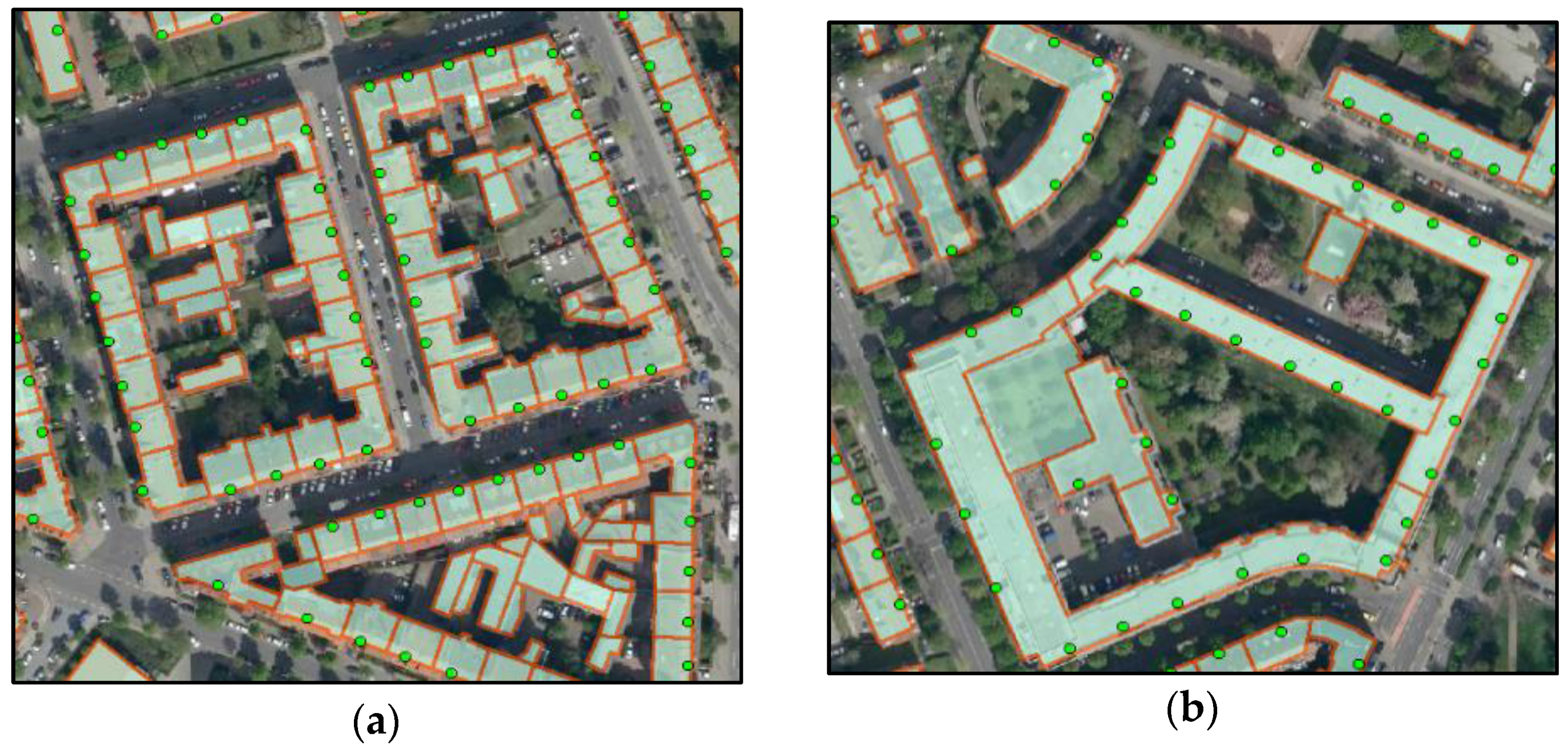
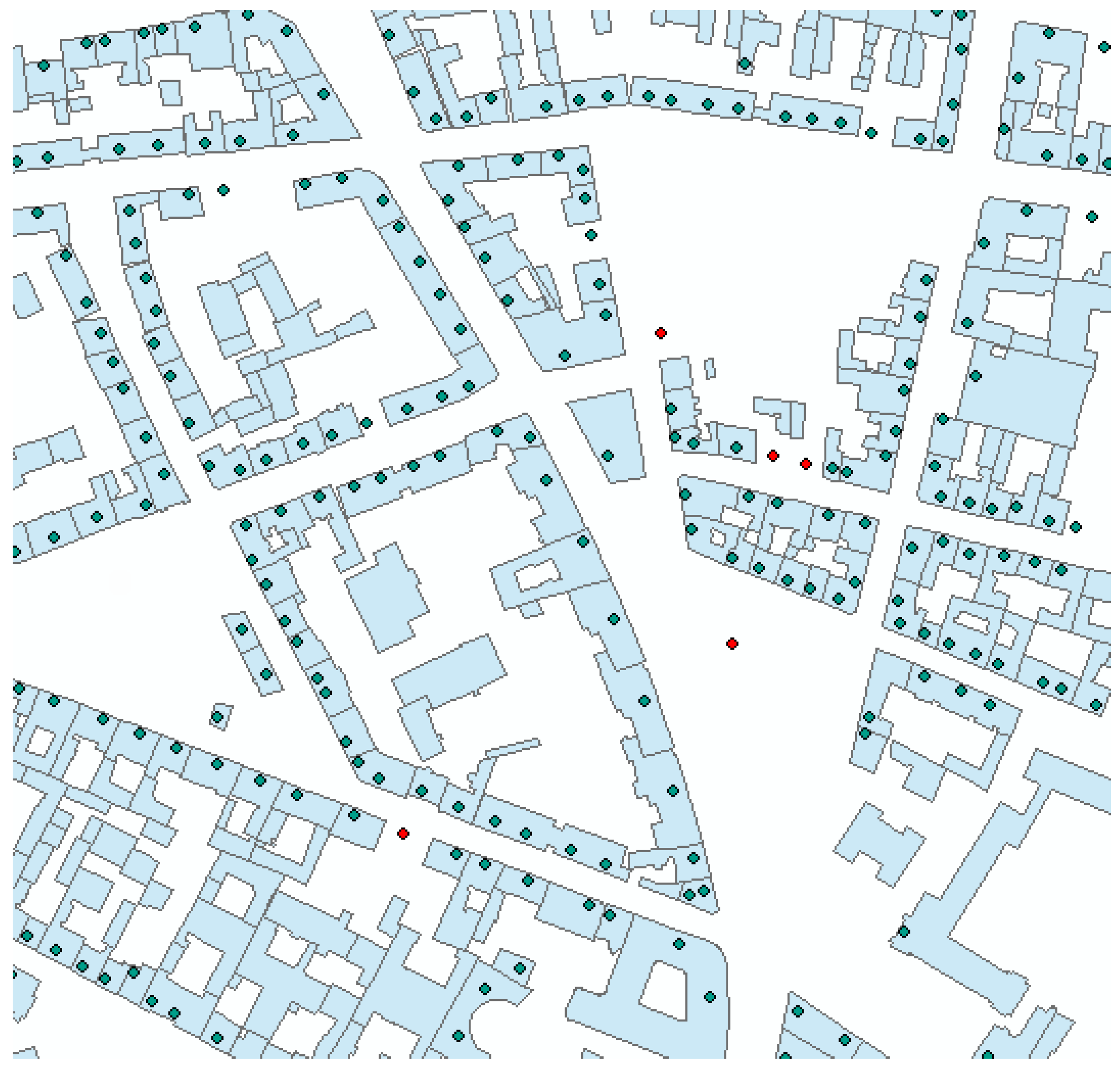
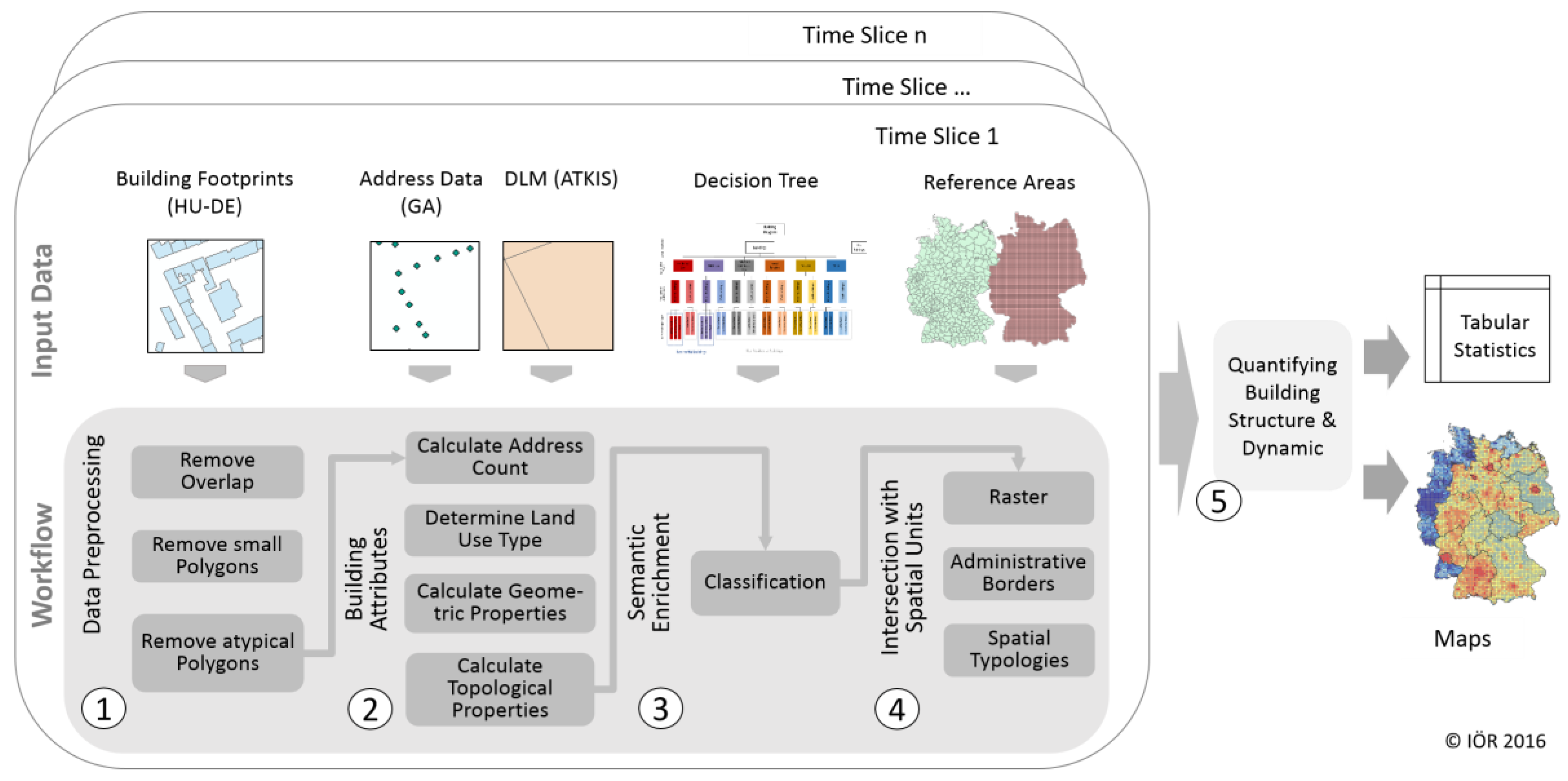
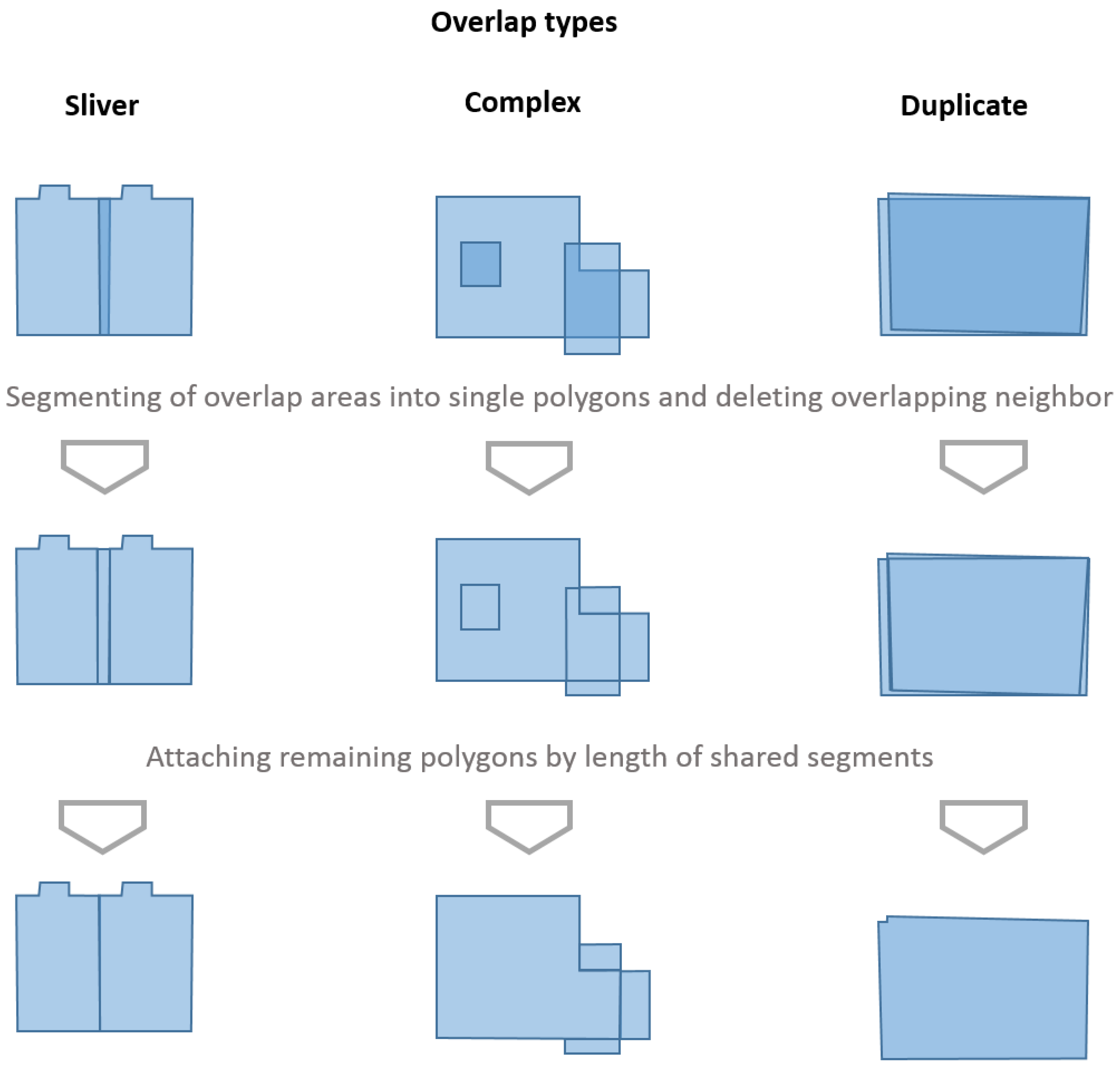
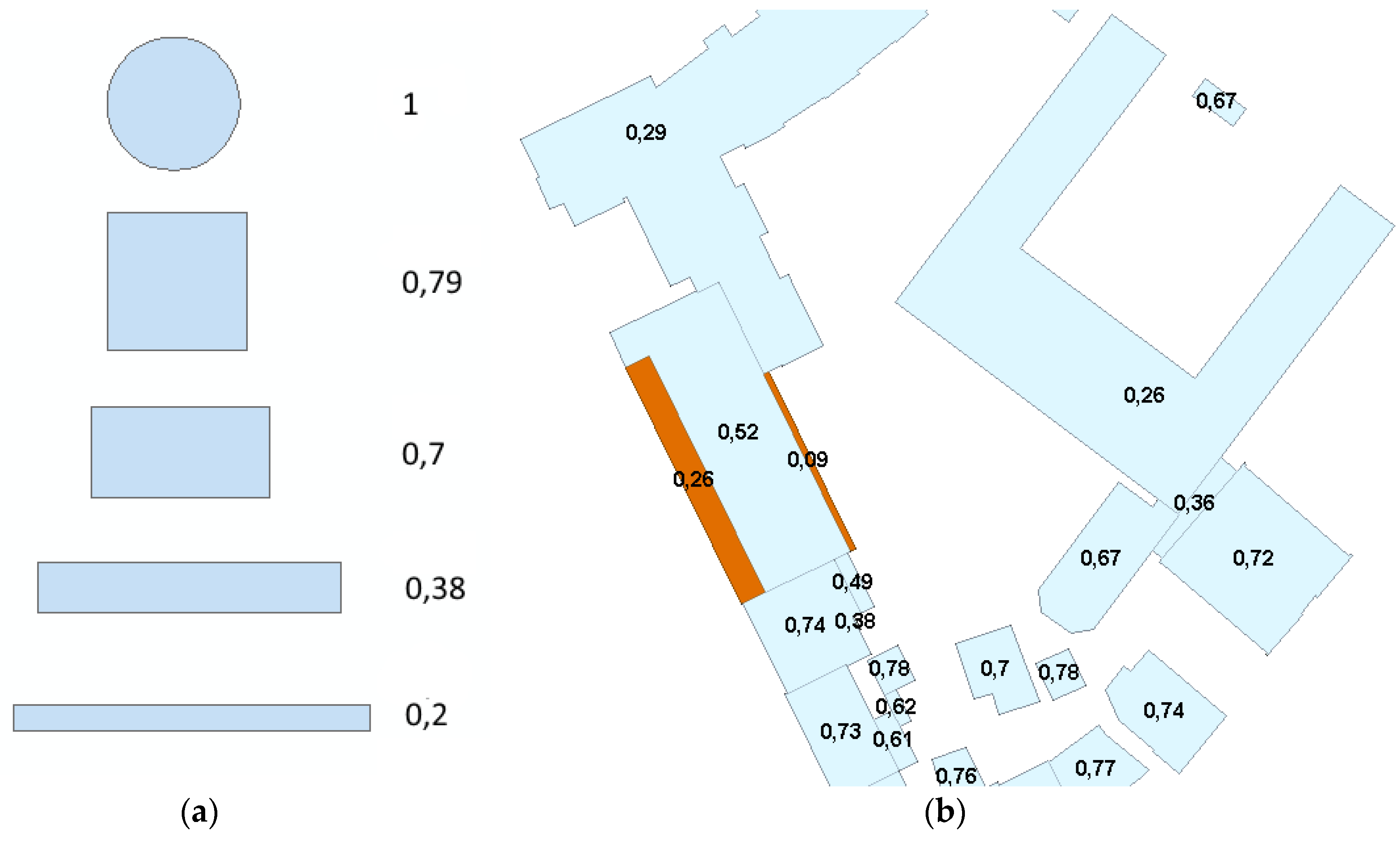
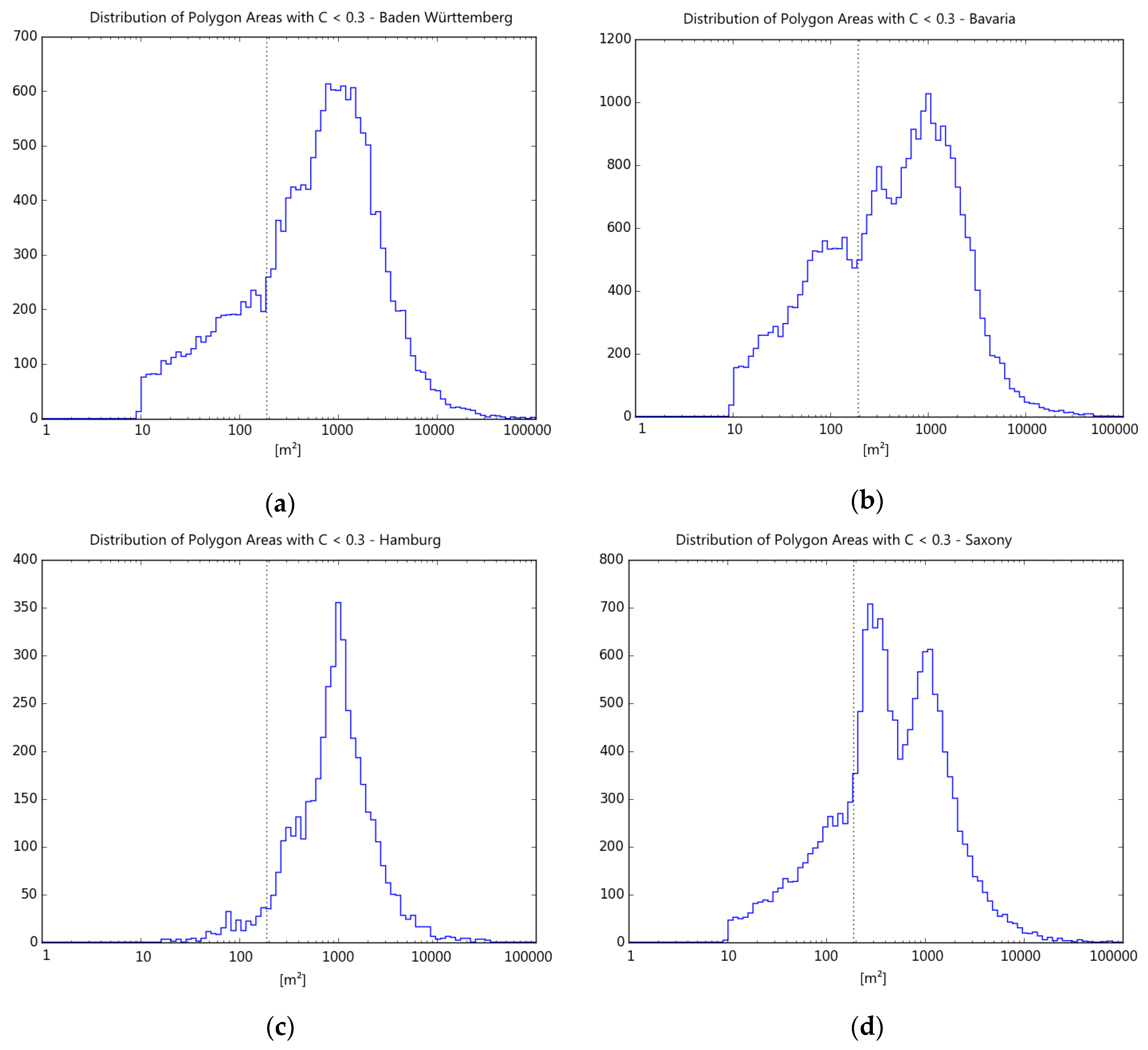
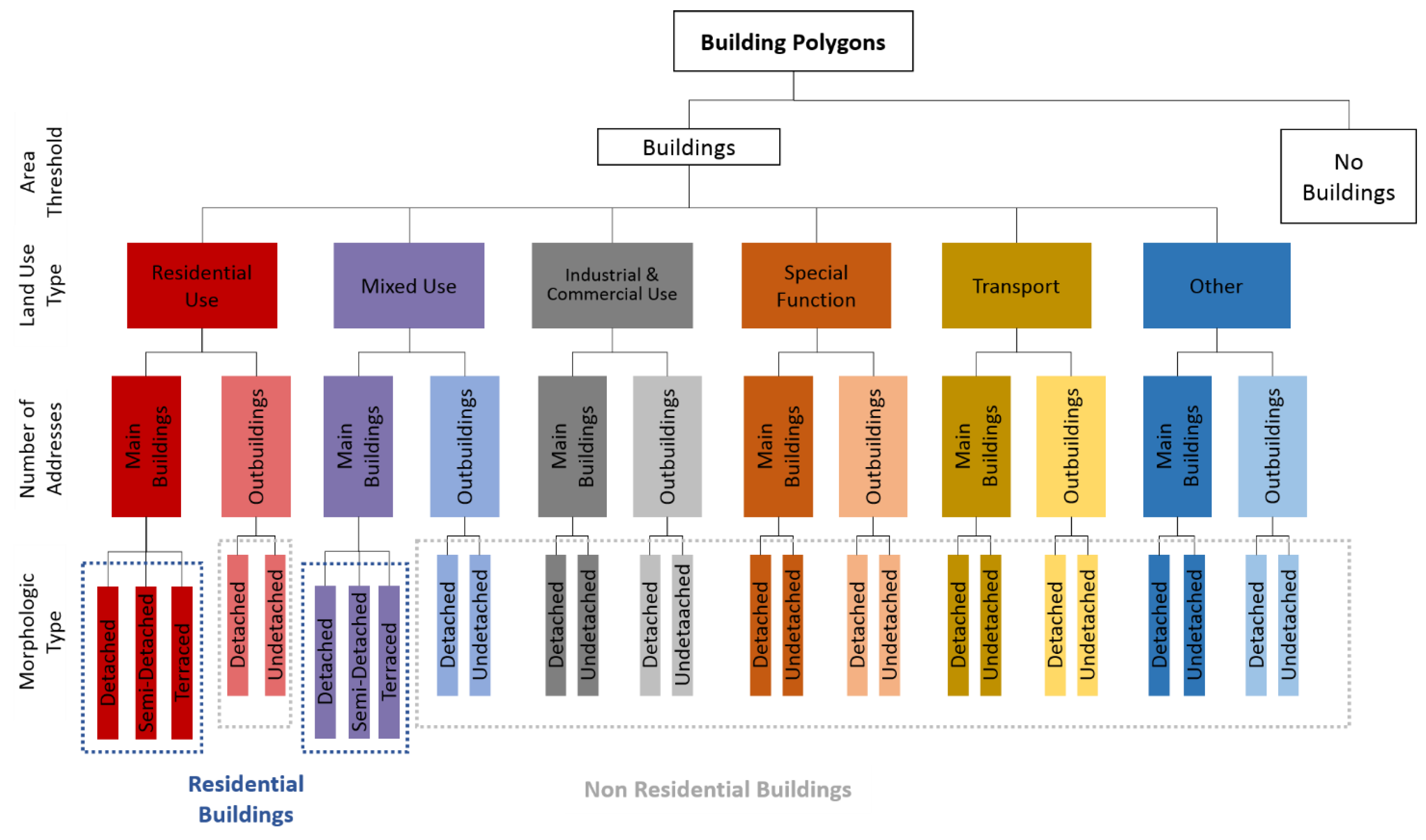
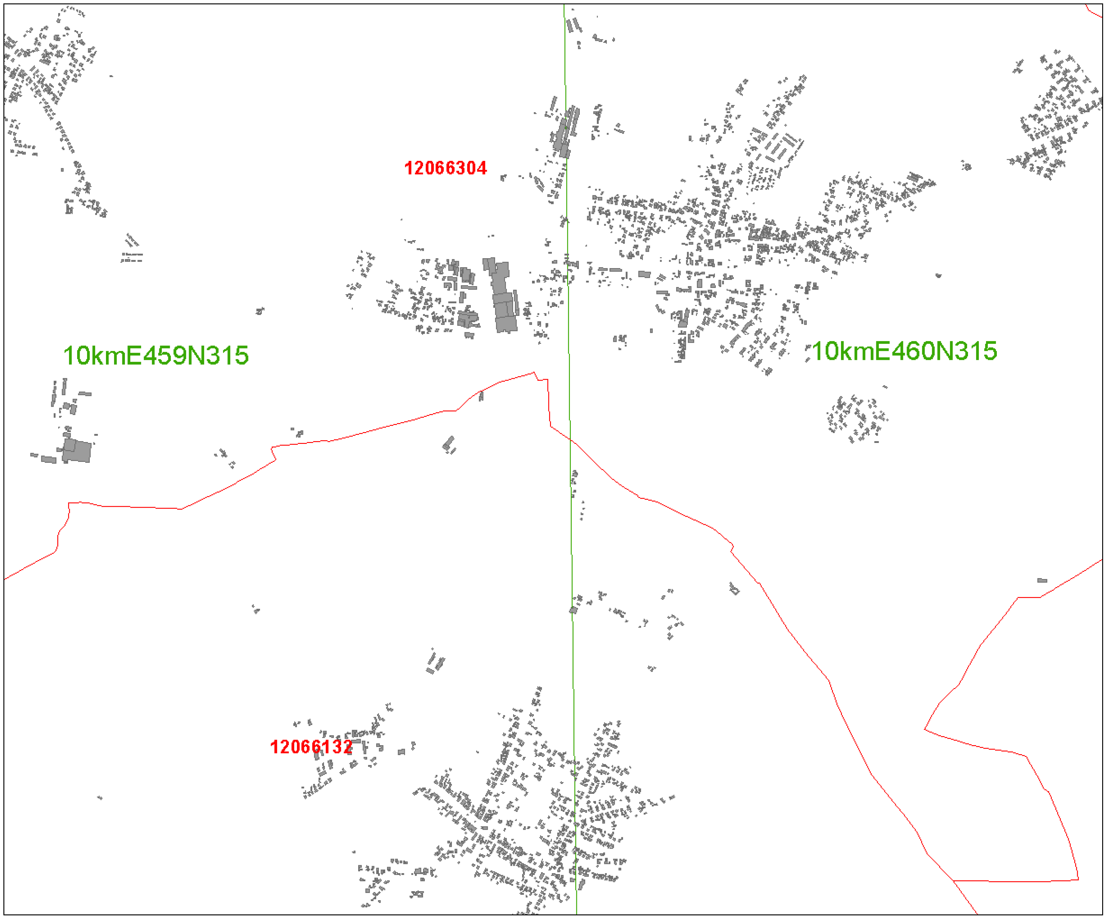
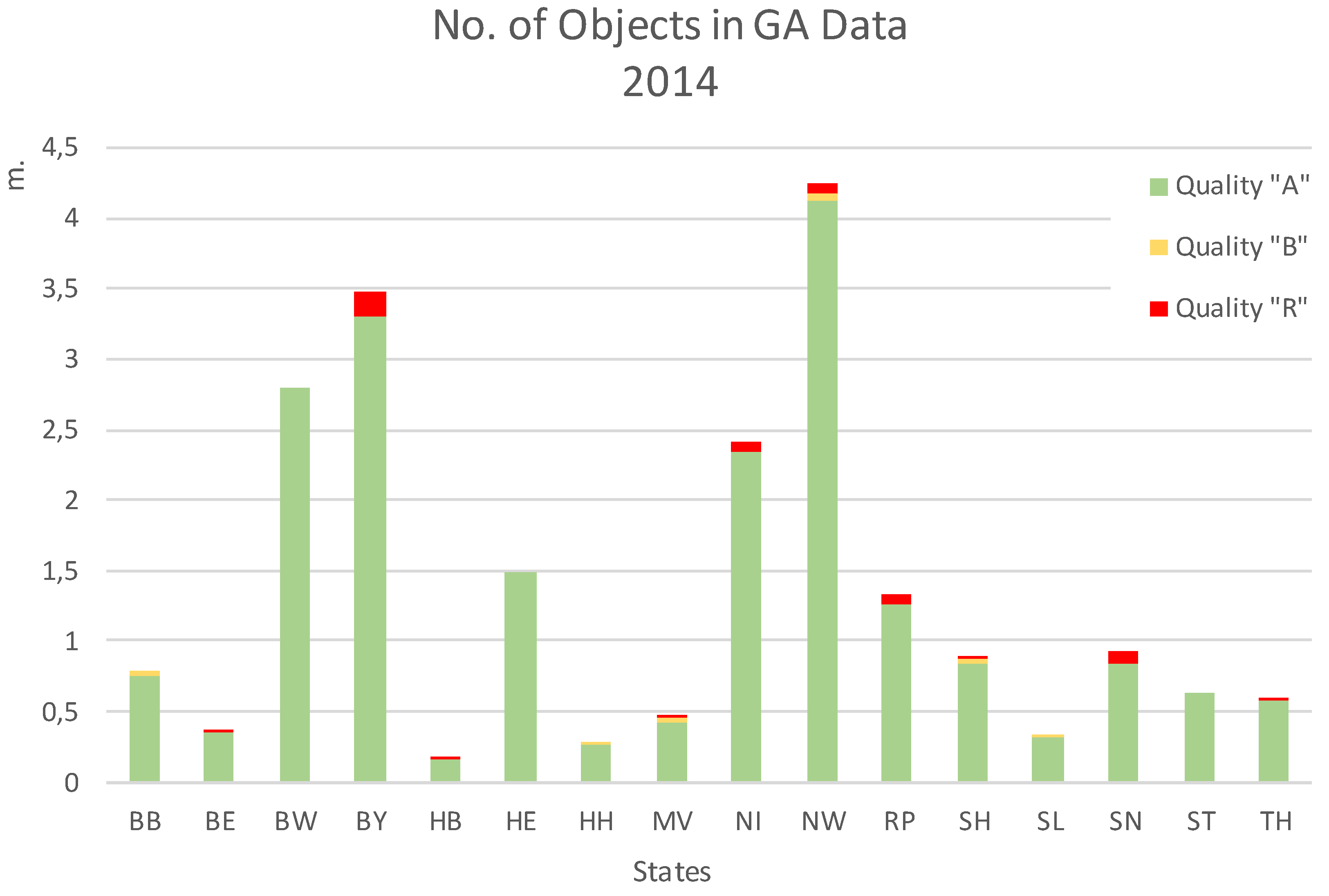
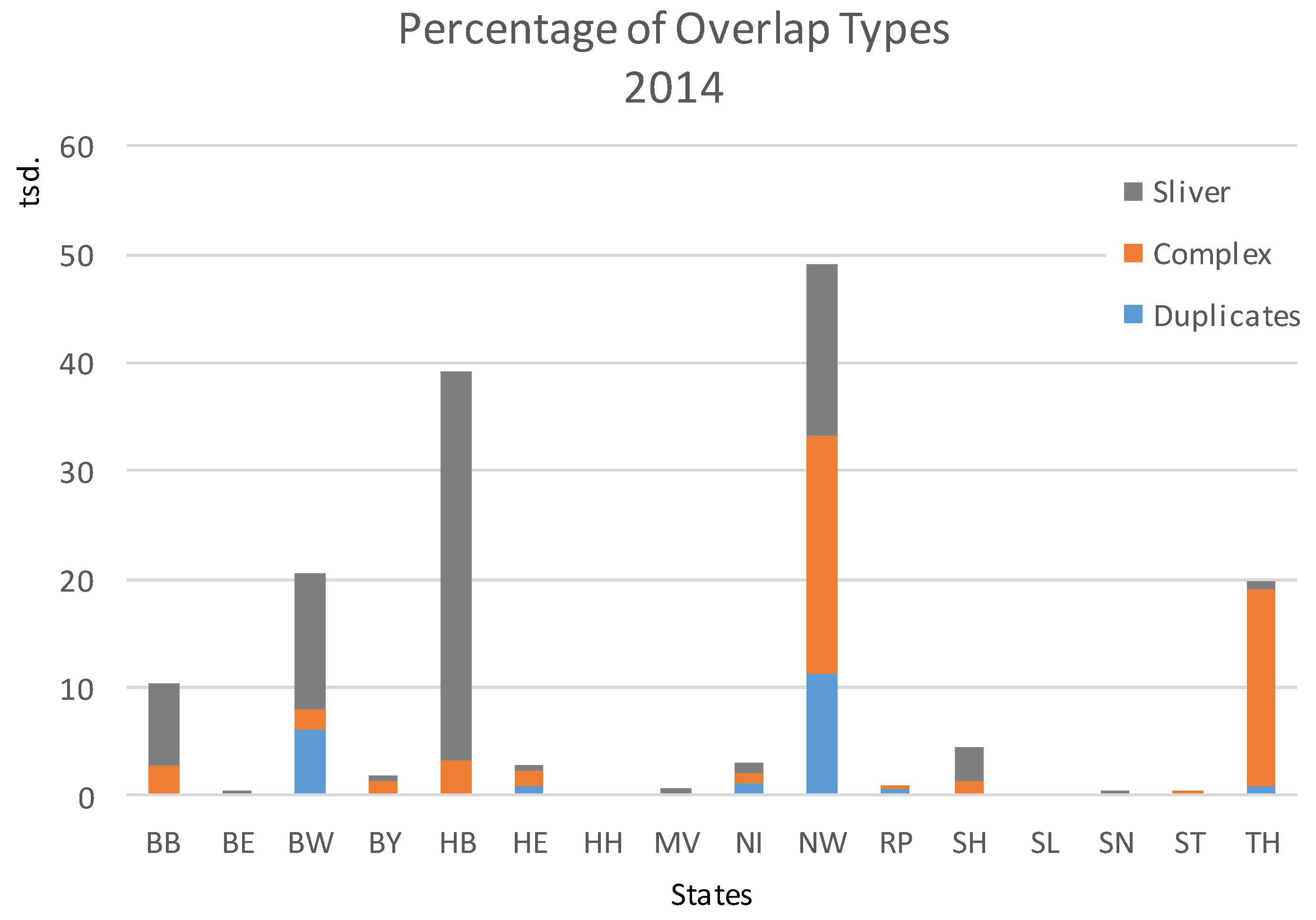
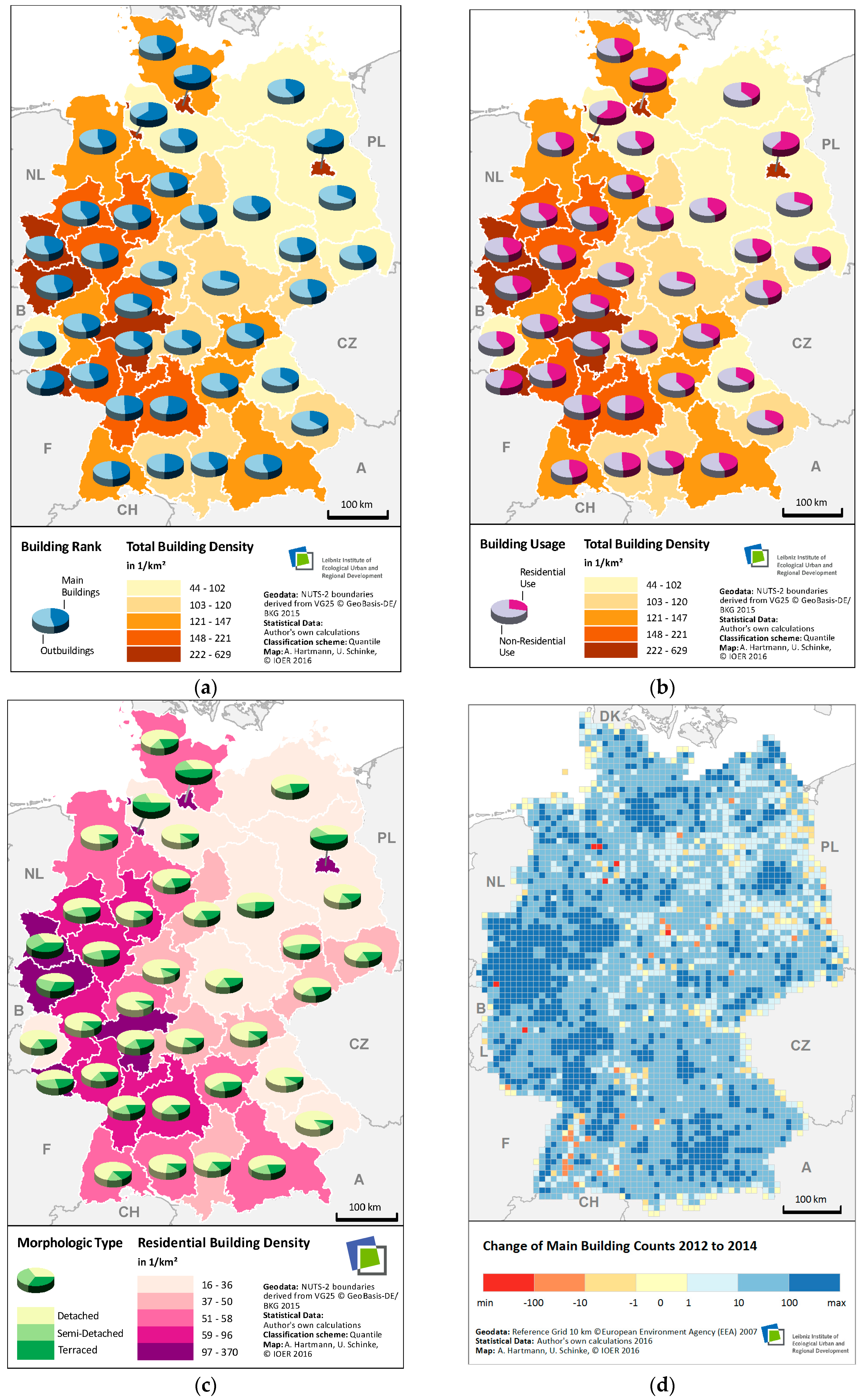
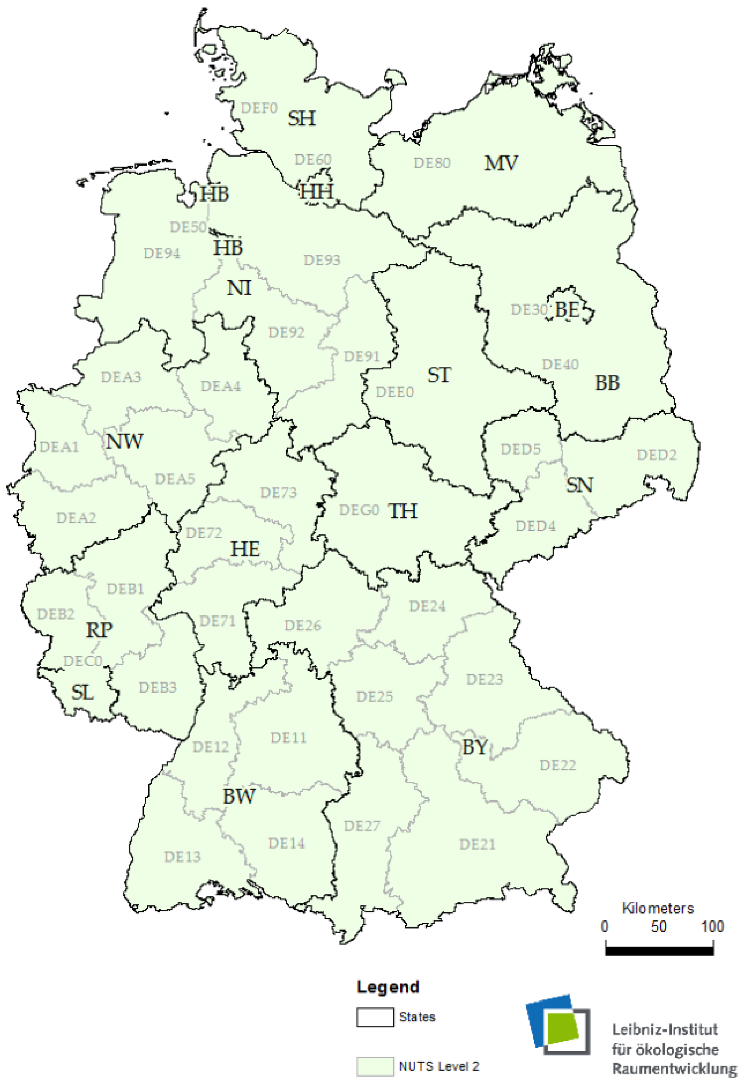