Methodology for Evaluating the Quality of Ecosystem Maps: A Case Study in the Andes

Abstract

Uncertainty in thematic maps has been tested mainly in maps with discrete or fuzzy classifications based on spectral data. However, many ecosystem maps in tropical countries consist of discrete polygons containing information on various ecosystem properties such as vegetation cover, soil, climate, geomorphology and biodiversity. The combination of these properties into one class leads to error. We propose a probability-based sampling design with two domains, multiple stages, and stratification with selection of primary sampling units (PSUs) proportional to the richness of strata present. Validation is undertaken through field visits and fine resolution remote sensing data. A pilot site in the center of the Colombian Andes was chosen to validate a government official ecosystem map. Twenty primary sampling units (PSUs) of 10 × 15 km were selected, and the final numbers of final sampling units (FSUs) were 76 for the terrestrial domain and 46 for the aquatic domain. Our results showed a confidence level of 95%, with the accuracy in the terrestrial domain varying between 51.8% and 64.3% and in the aquatic domain varying between 75% and 92%. Governments need to account for uncertainty since they rely on the quality of these maps to make decisions and guide policies.

1. Introduction

Thematic maps are used throughout the environmental sector for research but mostly for supporting policy decisions and land planning. Ecosystem maps are also used to describe the spatial patterns of various types of ecological units and often to describe the extents of different ecosystem types for biodiversity conservation purposes [1], as well as quantifying, valuing and planning for ecosystem services [2,3,4]. However, before being used, any map should undergo a process of some kind of accuracy assessment [5] as a way of testing whether the data set values fall within some limits of reliability. This is of particular importance before making any decisions based on a map. Many examples of accuracy assessment have been developed for ecosystem [6,7] and land cover maps, which are mainly constructed from remotely sensed data [5,8].

Map accuracy assessment usually has a sampling design component, followed by a response design, and finally some type of estimation and analysis procedures [5]. For land-cover validation, Foody and Atkinson (2002) undertook a review of methodologies and identified trouble areas including the measurement precision, sampling type, error type and dimension, as well as the spatial distribution and error in evaluating the differences. In terms of ecosystem maps, Meidinger [6] was one of the first to propose a multiscalar protocol to determine the acceptability of a map through an unbiased statistical design of the map polygons and then an assessment of the thematic content with finer spatial resolution data and ground verification. Meidinger’s protocol proposed several steps including selecting the type of unit to be evaluated (either polygons or small areas), selecting the level of sampling, selecting the sampling size, conducting planning, scoring to determine the proportions of the map, during which the dominant mapping entity is corrected, and finally developing comparative tables such as confusion matrices.

Other accuracy assessments have been developed for vegetation cover within the Geosphere-Biosphere International Program, Global Land Cover 2000 [9] and Glob Cover, highlighting the high cost of map validation and the need to have a global protocol and data available [10]. Some of the proposed approaches include a stratified random mapping of 5 × 5 km units for global datasets and a follow-up design based on interpretation by local experts at a finer spatial resolution using, for instance, QuickBird data [5,10]. A recent article [7] discusses uncertainty in ecosystem mapping by remote sensing and reviews some of the methods available, including fuzzy set theory, spectral unmixing and other alternative approaches based on Bayesian theory, maximum entropy or multivariate analysis.

The application of the methods is even scarcer in the literature, and most of the examples use remote sensing data or validate only the remotely sensed derived data even when assessing thematic maps. The global land cover [9] was validated using a cluster analysis for only three classes—forests, agriculture land and wetlands—choosing the proportion of pixels to be validated according to the class proportion of the map and reporting a general accuracy of 68% of the map using confusion matrices [11]. In South America, using stratified sampling, the land use and land cover map was validated using 26 sites per type of land cover after first eliminating macroscopic errors on polygon limits and labels [12]. A separate study on Latin America and the Caribbean [13] focused on land use changes from 2001 to 2010. They used visual interpretation of fine resolution images from Google Earth, Digital Globe’s QuickBird and IKONOS as reference data for the accuracy assessment and applied it to a sampling grid, providing error matrix analysis including details of producer (omission) and user (commission) error. The overall accuracy was 80.2% ± 8.1%, with a minimum of 65.1% in the Caribbean and a maximum of 97.1% in the savannahs of Uruguay.

Other than global and regional approaches, most of the Latin American local experiences of map validation are focused in Mexico, Peru, Ecuador and Argentina [14,15], but even there, sometimes despite field validation (plots, transects or rapid assessments), the accuracy of the map is not reported. In Venezuela, one study [16] reported the validation of a map of savannah ecosystems with field sampling areas of 1 km and had an overall accuracy of 90%, while the accuracy for hyper-seasonal and seasonal savannahs was 75%, and that for semi-seasonal savannah was below 50%.

Colombia has some tradition of constructing maps of land cover and ecosystems, but most do not include validation [17,18]. Two subnational maps, for the Andes and the Orinoquia [19,20], adapted Meidinger’s (2003) protocol for accuracy assessment of ecosystem maps to tropical conditions using fine resolution satellite data and field validation, and reported a global accuracy and a stratum accuracy per biome type.

Mapping complex ecological units as ecosystems is a process that has changed over time, and although remote sensing is an important part of these processes, other abiotic and biotic components of ecosystems are often incorporated. The Colombian ministry of environment and sustainable development, along with the research institutes, have been working on ecosystem mapping at a regional scale as an important contribution to land planning, and to provide scientific information for wildlife management [21]. With the purpose of fulfilling these objectives, an update of the ecosystems map at a scale of 1:100,000 was carried out, from the identification, classification and characterization of the ecosystems as a way to understand the territory. This process consisted of a bibliographic revision of the different identified, charted and investigated land and aquatic ecosystems in the country, to obtain a general typology [21]. Following this, a classification of the natural and transformed ecosystems was done, and natural ecosystems were identified by characteristics such as: weather, geopedology and cover. Posteriorly, ecosystems were grouped and classified in synthesis units in accordance with the limit variables named before, resulting in a hierarchic legend which relates the ecosystems’ components [21]. However, governments need to know the quality of the information on which they are basing their decisions. This paper presents the development and application of a methodology to validate the quality of the official ecosystem map in Colombia, applying this methodology to a pilot site in the Andean region. The pilot region is characterized by different altitude, geomorphological and transformation gradients with ecosystems converging from both upland and lowland areas. The objectives of this work are to develop and apply a selected sample and response design using fine resolution images and field validation data and to assess the thematic accuracy of the results.

2. Methods

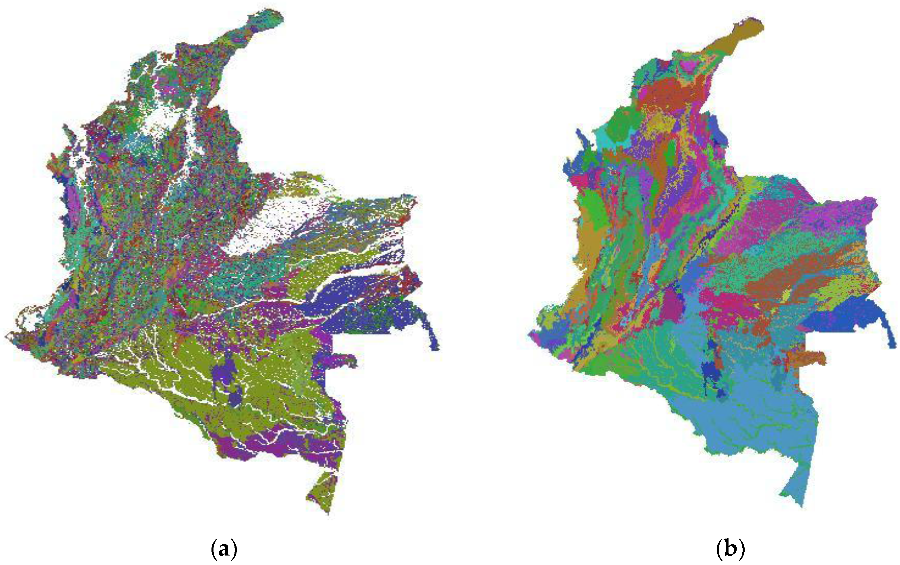
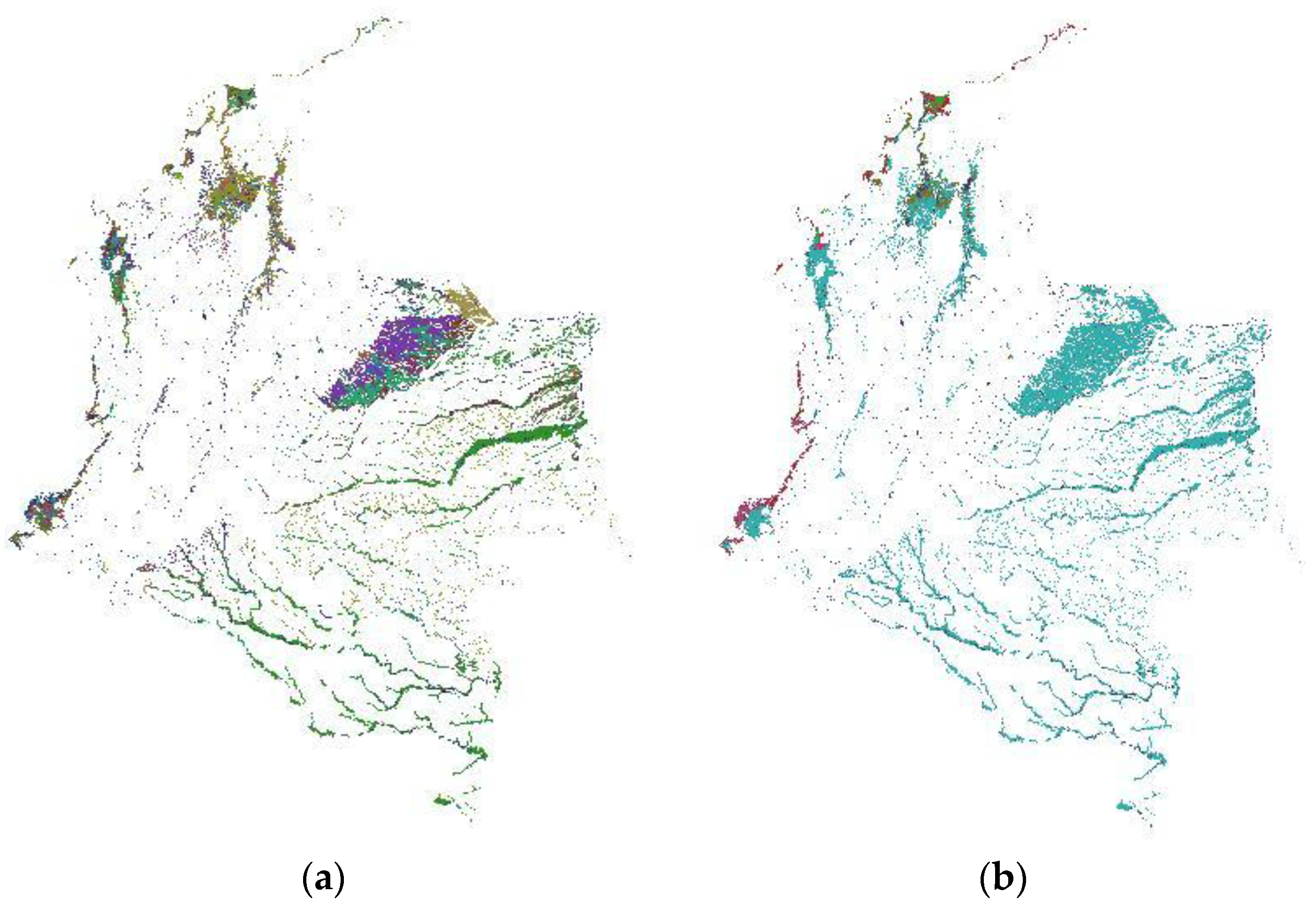
2.1. Ecosystem Map

The Colombian ecosystem map (scale 1:100,000) contains terrestrial and aquatic ecosystems information [21] and uses a vertical structure [22] that combines and relates both biotic and abiotic components in a hierarchical way [23]. Overall, this map reports a total of 3930 ecosystems (Figure 1a), grouped into 274 biomes for the terrestrial domain (Figure 1b) and into 5878 ecosystems (Figure 2a) contained within 625 types of general ecosystems (Figure 2b) for the water domain.

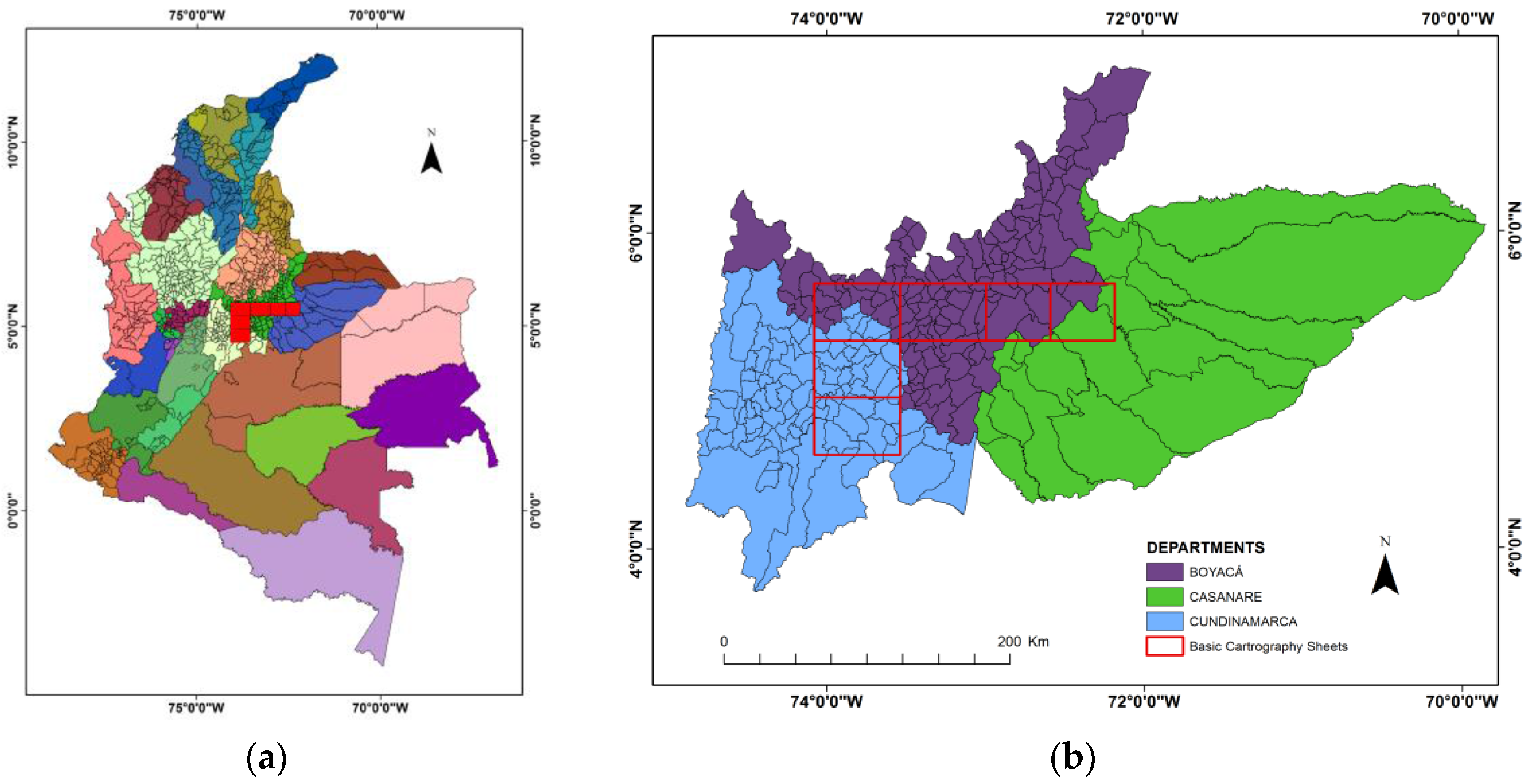
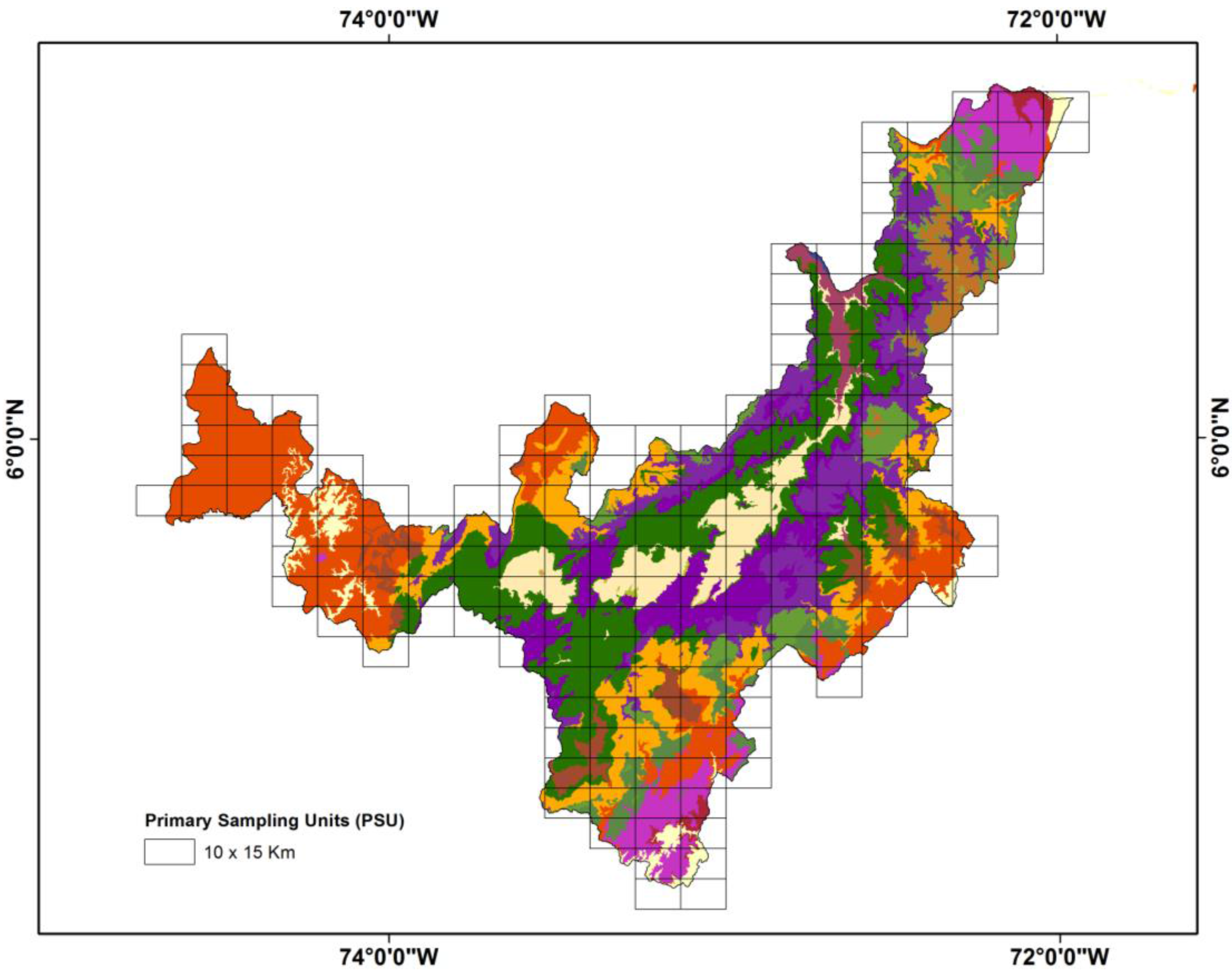
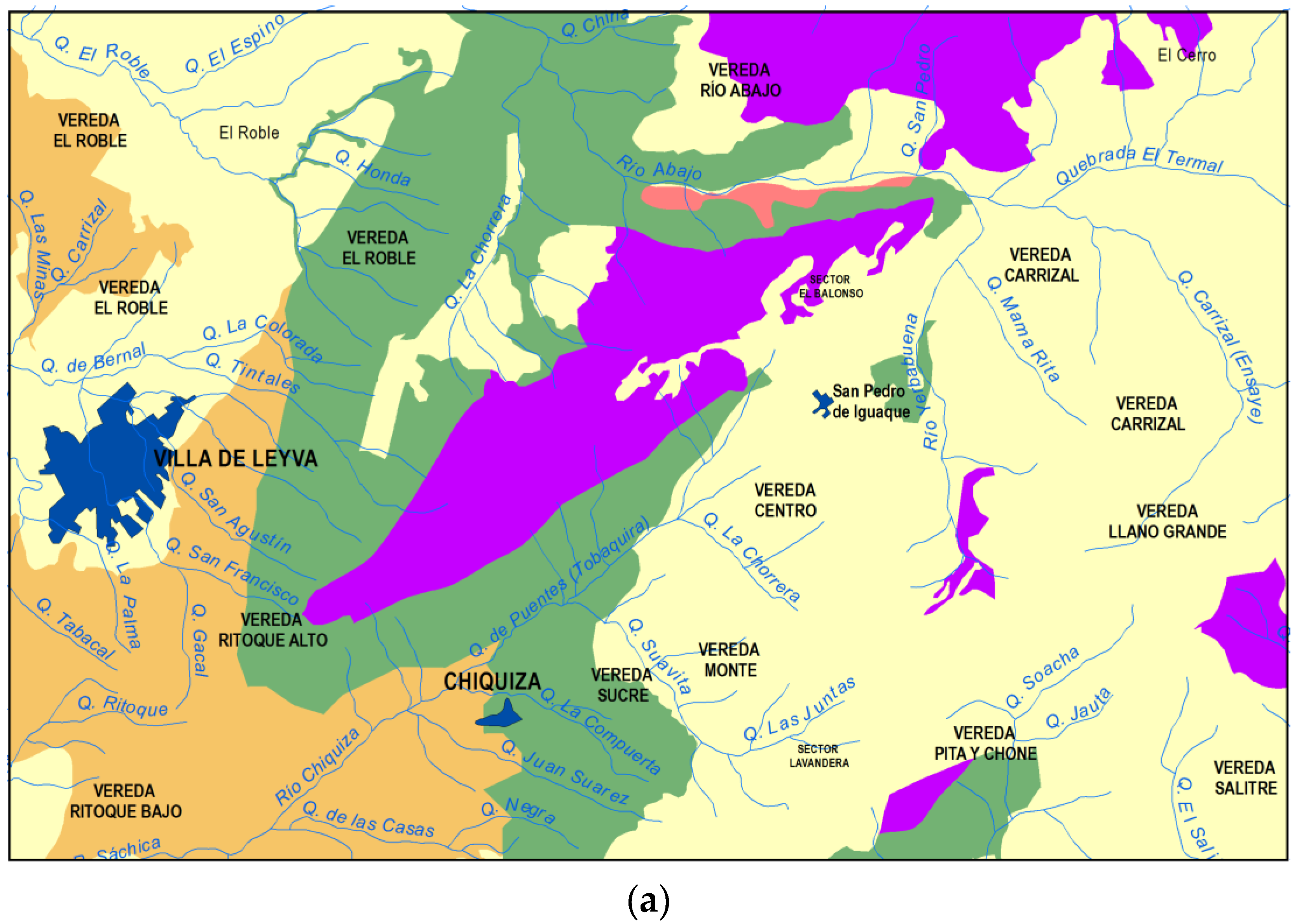
2.2. Pilot Study Site

The validation was performed on a window located in the central Andes in the departments of Cundinamarca, Boyacá and Casanare, covering six sheets at 1:100,000 (Plates 190, 191, 192, 193, 209 and 228) and an area of 1,501,709 ha. This window was selected with the assistance of officers from IDEAM, the producing institution, and is located in a terrestrial strategic area that includes ecosystems of the Andean region, specifically in the Eastern Mountain Range and some Orinoco lowland ecosystems, both terrestrial and aquatic (Figure 3).

The region comprises the Andean system belonging to the Eastern Cordillera and is characterized by a variety of thermal floors that give a temperature gradient ranging from 32 °C in the equatorial zone to 2 °C in the Páramo region [24], and moisture regimes from superhumid to dry with or without water deficit, with tendencies toward minimal or very high changes in temperature depending on the region. The selected pilot window contains 994 terrestrial ecosystems, which represent 25.3% of the terrestrial ecosystems identified in the national territory and are grouped into 20 biomes, and 107 aquatic ecosystems representing 1.82% of those reported for the country, contained in eight functional subsystems, all of them continental (Figure 3).

2.3. Sampling Design

Areas for probability sampling with two domain and multiple stages were established, and stratified with selection proportional to the richness of strata present in each primary sampling unit (PSU). These strata are defined geographical units limited by biomes for the terrestrial domain and functional subsystems for the aquatic domain. For purposes of logistics associated with the optimization of financial resources, the selection of the sample includes the following stages.

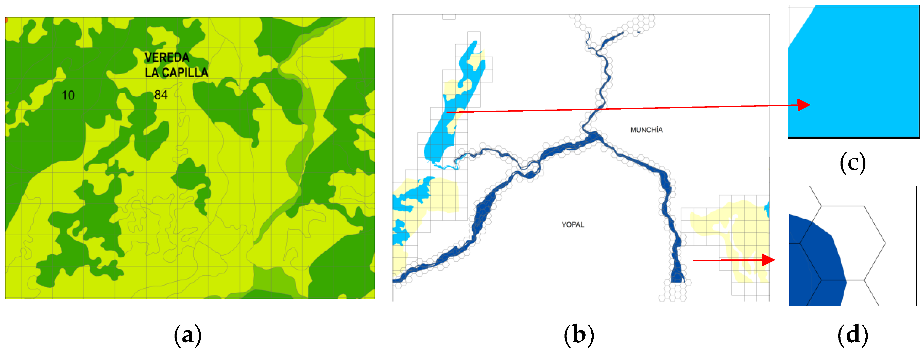
2.3.1. First Stage

Primary Sampling Units (PSUs) were selected at the country level, each consisting of a rectangular geographical area of 10 km × 15 km (150 km²), corresponding to 1/16 units with a scale of 1:100,000 (Figure 4).

The random sampling was adjusted using the probability derived from the number of strata and ecosystems contained in each PSU; thus it is most likely to choose those PSUs that have the most diverse strata (Figure 5).

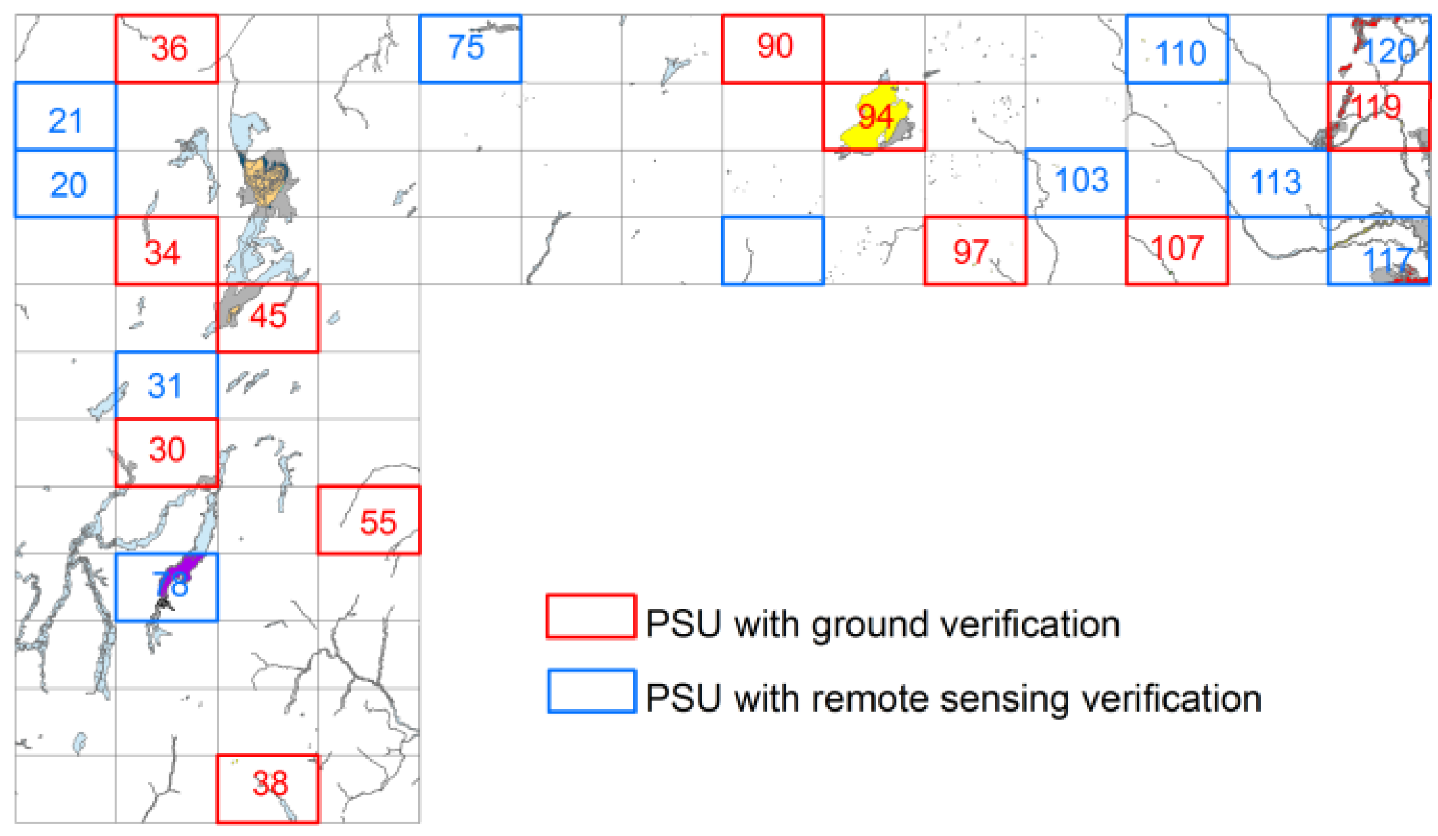
2.3.2. Second Stage

Final Sampling Units (FSUs) or reference units are the spatial unit that serves as the basis for the comparison of the reference classification and the ecosystems map. The size and shape of each FSU correspond to squares of 25 ha for the terrestrial domain and to hexagons of 5 ha in the aquatic domain in lotic and lentic subsystems, whereas the transitional and transformed aquatic units also used squares of 25 ha (

Table 1. Size of the final sampling unit (FSU) or reference unit.

Stratum	Ecosystem Richness	FSU Size (ha)
Terrestrial Domain
Lithobiome of the high plains, Amazonian Plain	10	25
Lithobiome of the high plains, floodplains, Guiana shield	11	25
Transformed	264	25
Stratum	3582	25
THZ of the Magdalena River Delta, Eastern Mountain Range	57	25
THZ of the alluvial valley, the Atrato and San Juan Rivers, the Serranía del Baudó, and the coastal plains of the Pacific	6	25
Aquatic Domain
Andean Atlantic Lentic	7	5
Andean Atlantic Lotic	7	5
Andean Atlantic Transitional	24	25
Artificial	3	5
Transformed	84	25
Stratum n	5734	25
Old lentic platforms	1	5
Old lotic platforms	6	5
Old transitional platforms	12	25

). These areas correspond to the minimum mapping units included in the National Ecosystem Map are sampled within each stratum contained in the selected PSUs.

Given the characteristics of the main land mass of the ecosystem map, the observation unit can be constituted by a transect (subsample of the FSU), an observation of the entire FSU or plot size defined according to the type of layer used to validate the response design. Finally, the following criteria were met:

• Each FSU belonged to a single stratum.
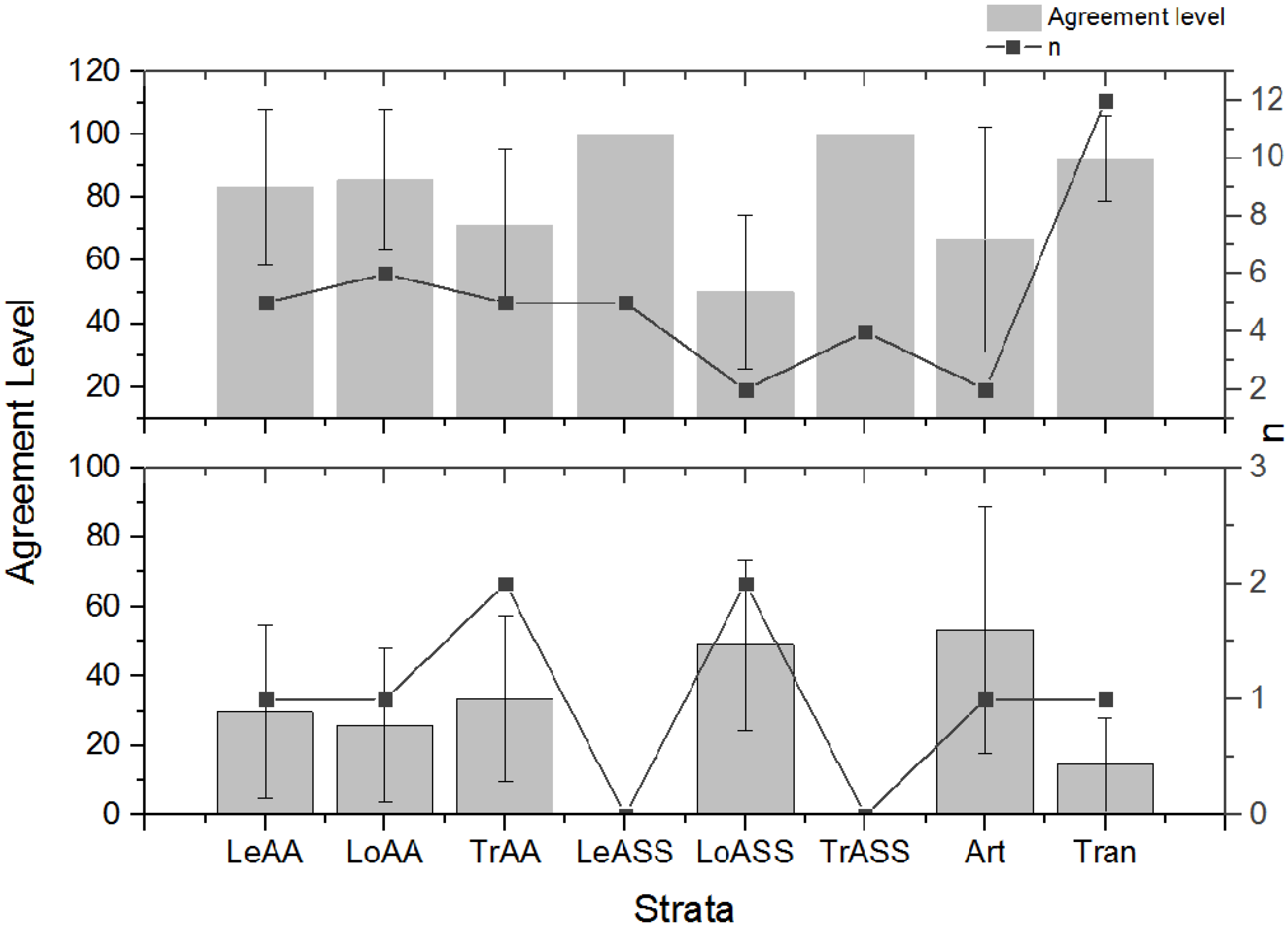
• The sample size for each stratum (n) was proportional to the ecosystem richness in each biome or subsystem.
• To consider each biome/functional subsystem as a stratum, it is required to have a minimum of 3 final sampling units (FSUs) which allows to obtain an estimate of the sampling error.
• The transformed ecosystems were grouped into one stratum for both terrestrial and aquatic domains.
• The selection of FSU (spatial distribution) was based on randomness.
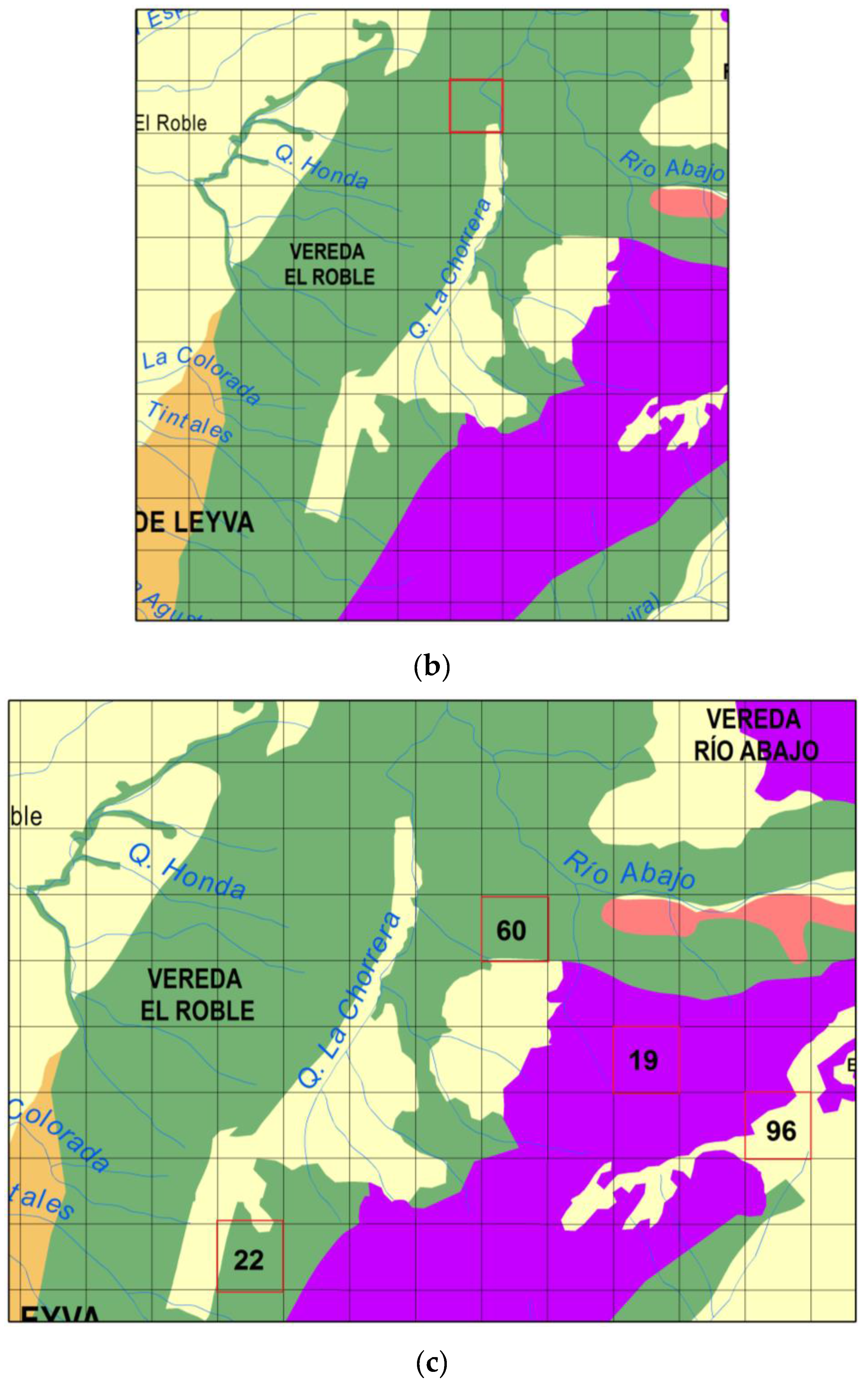
• Each selected FSU had to contain more than 80% of the stratum to be validated. If the first selected FSU did not meet this requirement, a second FSU was selected in order to meet the proposed sample size for each stratum. When a FSU had several ecosystems within the stratum to validate, it was necessary to evaluate each ecosystem and to assign an agreement to the reference unit.

2.4. Sampling Size

The sample size is the number of ultimate final sampling units (FSUs) necessary to estimate the reliability of the map. The following formula was used:

$$n =\frac{p x q t_{\alpha /2}^2}{e^2}$$

(1)

where

• n is the number of FSUs to evaluate
• p is the number of units classified correctly
• q is the proportion of units classified incorrectly
• t is the abscissa of the t distribution for a 95% confidence
• e is the relative error of 5%

The FSUs are randomly selected to meet the required number for each stratum, i.e., the estimated n. Once the PSU is selected (Figure 5a), a division of the strata was made (FSU) (Figure 5b), and finally the FSUs were randomly selected (Figure 5c). For the aquatic domain and the transitional subsystem, the same process was undertaken (Figure 6a–c); however, for the lotic and lentic subsystems, FSUs correspond to hexagons (Figure 6b–d). Material for testing was prepared from the appropriate sources of reference.

2.5. Data Sources and Validation

The FSUs can be evaluated using various sources of information, and the chosen method or methods must be consistent with the purpose of assessing the accuracy, time and resources available to carry out the process. Several sources are listed in order of importance (

Table 2. Information sources for reference data recommended for the validation process.

Data Sources	Characteristics	Example
Field work	Field data collection to fill validation formats.
Medium-resolution satellite images	Landsat 7 ETM (30 m) SPOT-4 multispectral (20 m) SPOT-4 panchromatic (10 m)
Fine resolution satellite images	Ikonos panchromatic (1 m), multispectral (4 m) Aster Airborne multispectral scanners > 0.3 m CBERS 1–3, Geoeye Lidar, QuickBird Worldview
Thematic cartography	Soil maps of Colombia Scales of 1:100,000 to 1:25,000 [25] Map of Paramos in Colombia, scale 1:100,000 [26] Map of dry forests distribution in Colombia, scale 1:100,000 [27]. Wetland map for Colombia, scale 1:100,000 and 1:25,000 [28]
Floristic inventories or other data for species	Database of biological records from collections mainly of the Biodiversity Information System for Colombia (SIB), the Global System of Biodiversity Information Facility (GBIF) and specific project data (i.e., inventory of wetlands—MADS).

). These sources must be of higher quality than those used for mapping the ecosystem (finer resolution scale). If by some chance the same information source used for creating the map has to be used for validation, then the process used to create the reference classification must be more accurate than the process used to develop the map; and the date for satellite images used as reference sources must coincide with the year of the inputs of the classification, particularly in the land-cover component.

2.6. Field Data

Field data represent the most accurate way to measure the reference classification source. The field data collection is based on pre-established methodologies developed by a group of experts in the field. Generally, the evaluation is done by observation, sampling transects or plots randomly distributed within each selected FSU.

Two field trips were conducted during the month of November 2014; the first in the area of the Altiplano Cundiboyacense (Cundinamarca and Boyacá high plateaus) and the second in a sector of the piedmont and eastern slopes of the Eastern Mountain Range (Casanare and Boyacá). The PSUs were randomly selected, like the selection of the FSUs, considering the rich strata within each PSU, in order to optimize logistics and time resources during the verification process. The field material per PSU for the reference classification consisted of the following:

-

Basic Cartography: information on location of paths, roads and rivers to facilitate the location and access to the FSU.

-

Cartography corresponding to the selected PSU using Landsat images from 2008 (reference date of the land-cover map used in the original mapping ecosystems) and RapidEye images from 2010 for the location of each FSU.

-

Additional cartographic material such as ecosystems in each FSU and map of edaphogenetic environments.

-

Field formats.

-

GPS Garmin62sc (Garmin, Lenexa, KS, USA), Munsell chart, pH metre and reagents for testing some edaphogenetic characteristics.

-

Satellite images: Data obtained from satellite imagery can be relatively inexpensive and an easier alternative application in hard to reach areas, complementing the field validation process. Such an assessment must be performed by an expert in the subject, and the uncertainty and variability of the data should be considered through clear evaluation criteria. Either intermediate resolution images such as Landsat and SPOT or fine resolution images can be used. The images used for the pilot correspond to the Landsat 7-56200801-02, 8-56 and 8-572007/02/232007/02/07, a fine resolution Rapideye of 2010 was also used and in some cases Google Earth consulted.

-

Cartographic information and additional data bases: Other supporting data can provide useful sources of reference in the first level of classification of ecosystems, e.g., projects at national and regional level that are being carried out in the country. Available information for Páramos [26], dry forests [27], wetlands [28], fauna and flora inventories was used.

For this assessment, the selection of two to three FSU for each stratum were evaluated in the PSU, validating one or two FSU at most.

Finally, to define the rules on the agreement of the classification map versus the reference classification, the variables that define both strata and ecosystems were prioritized. First the stratum is evaluated, and once there is agreement between the classifications, the ecosystem or ecosystems contained within that stratum are then evaluated. If there are two or more ecosystems within the PSU, its presence is first validated to indicate the percentage occupied by each ecosystem. If it is not possible to identify this in the reference classification, the entry is made by validating the ecosystem with the highest percentage in the stratum. To reach “agreement” status, at least 70% of the area of an ecosystem must be occupied by the variable that characterizes it.

2.7. Analysis

The estimation of the overall proportion of the well classified PSUs and the accuracy were quantified by standard errors, using the following formulas:

$$\widehat{p} ={\displaystyle \sum }_{h=1}^H{W}_h{P}_h$$

(2)

where:

• $\widehat{P}$ is the sample proportion of FSUs correctly classified in the map
• $P_h$ is the proportion of PSUs correctly classified in stratum
• $W_h$ is the FSU proportion that belong to the stratum
• H is the weight associated with each stratum
• W_h and H are determined by the relationship between the number of FSU in each stratum and the total number of FSU in the map (proportion of units classified incorrectly)

$$=z \sqrt{\frac{1}{N^{2 }}{\displaystyle \sum }_{H=1}^H{N}_h^2}\frac{N_h-n_h }{N_h}\frac{p_h{q}_h}{n_h-1}$$

(3)

where:

• $\in :$ standard error
• Z: 1.96 (95% confident)
• N: total number of UFM in the map
• N_h: total number of PSU in stratum h
• n_h: number of PSU in stratum h of the sample
• q_h: represents the proportion of PSU classified incorrectly in stratum

3. Results and Discussion

A total of 22 PSUs were selected (Figure 7 and Figure 8), and a total of 76 FSUs for the terrestrial domain and 46 for the aquatic domain (Figure 9 and Figure 10, Tables S1 and S2). In the terrestrial domain, 34 out of 76 of the validated FSUs did not match the legend given by the map. Therefore, with a confidence level of 95%, the labelling of single domains in the map of the terrestrial ecosystems only ranged between 51% and 64% accuracy (Figure 9). For the aquatic domain, only 8 out of 46 of the validated units did not match the legend; with a confidence interval of 95%, the accuracy for the aquatic ecosystems ranged between 75% and 92% (Figure 10, Table S2).

The confidence intervals for our results can still be considered too large, but because only a pilot area was used to test the methodology, we believe that our results are a good indicator of the quality of the map. Indeed, more extended strata are easier to evaluate, and their level of agreement is high, whereas azonal strata, which are rare within the pilot window, yielded less favourable results, e.g., Andean Aazonal Orobiome of the Eastern Mountain Range and Altiplano Cundiboyacense strata (AAOEMR-AC) (Figure 9). This is partly due to the smaller number of FSUs (Figure 9) and the location within an anthropic matrix. Further, some of the common mistakes of the ecosystem maps are associated with errors from the source information used; such is the case with the land-cover map, where the label of a polygon does not tend to match the current or previous information condition of the reference year. This is most evident in areas with high land use dynamics, like the current area where the pilot window is located [29]. In addition, the high heterogeneity in some areas, in relation to the scale of the map, makes it very difficult to differentiate biomes and ecosystems. In this sense, it will be necessary to develop specific criteria to classify and evaluate both biomes and ecosystems. In this sense, the development of specific criteria to classify and assess biomes and ecosystems will be necessary, including spatial pattern information [30], and thus distinguish the ecosystems highly influenced by anthropic pressures among the regional matrices, or small ecosystems restricted by physical factors or local dynamics.

On the other hand, azonal Andean ecosystems and azonal Páramos are difficult to identify due to their high level of anthropic intervention processes [29]. This has caused soil changes and the establishment of a series of ecosystem successional stages. Thus, some characteristics of these ecosystems vary considerably even in nearby sites, and it is very complex to identify the reference unit, as there are no specific parameters in these cases. Therefore, the recommendation is to consider the FSUs of these subsystems as a single transitional layer and to focus future efforts on better characterization. These are key sites for which future policy efforts should focus on restoration and conservation.

The FSUs of the sub-Andean biomes of the Eastern Mountain Range and the high plains also have a very low agreement, probably due to the high levels of intervention. There were some errors on the altitudinal limit defined in the methodology. We suggest the establishment of a minimum size of altitudinal ranges for acceptable sampling units in these transitional areas, and that size should also be associated with the slopes of each mountain range.

The ecosystem map is the result of a combination of formation factors organized in a hierarchical fashion, and, for the terrestrial domain, the ecosystem spatial unit must consider the incorporation of the floristic aspect. From this perspective, it is necessary to incorporate into the ecosystem mapping process modeling methods to identify the emergent properties of the ecosystems, where a group of plant communities coexist among heterogeneous landscapes, meaning more functional ecosystem units are mapped.

Specifically, for the aquatic domain, it is recommended that the transitional ecosystems are considered as an amphibious domain, because these zones gather characteristics of both domains, aquatic and terrestrial. The river landscape integrity for the lotic stratum and the mean depth of the lentic stratum are variables that explain the dynamism of these systems, and its incorporation into the mapping process strengthens the delimitation and characterization of the ecosystems’ units.

Finally, the fact that a government conducts this type of quality assessment for the information produced by official institutions is a key step to make better decisions regarding ecosystem conservation, ecosystem service valuation and, finally, land planning and management.

References

- Keith, D.A.; Rodríguez, J.P.; Rodríguez-Clark, K.M.; Nicholson, E.; Aapala, K.; Alonso, A.; Asmussen, M.; Bachman, S.; Basset, A.; Barrow, E.G.; et al. Scientific foundations for an IUCN red list of ecosystems. PLoS ONE 2013, 8, e62111. [Google Scholar] [CrossRef] [PubMed] [Green Version]
- Egoh, B.; Reyers, B.; Rouget, M.; Bode, M.; Richardson, D.M. Spatial congruence between biodiversity and ecosystem services in South Africa. Biol. Conserv. 2008, 142, 553–562. [Google Scholar] [CrossRef]
- Egoh, B.; Reyers, B.; Rouget, M.; Richardson, D.M.; Le Maitre, D.C.; van Jaarsveld, A.S. Mapping ecosystem services for planning and management. Agric. Ecosyst. Environ. 2008, 127, 135–140. [Google Scholar] [CrossRef]
- Crossman, N.D.; Burkhard, B.; Nedkov, S. Quantifying and mapping ecosystem services. Int. J. Biodivers. Sci. Ecosyst. Serv. Manag. 2012, 8, 1–4. [Google Scholar] [CrossRef]
- Stehman, S.V.; Czaplewski, R.L. Design and analysis for thematic map accuracy assessment—An application of satellite imagery. Remote Sens. Environ. 1998, 64, 331–344. [Google Scholar] [CrossRef]
- Meidinger, D.V. Protocol for Accuracy Assessment of Ecosystem Maps; Technical Report 011; Ministry of Forests: Victoria, BC, USA, 2003; p. 23. [Google Scholar]
- Rocchini, D.; Foody, G.M.; Nagendra, H.; Ricotta, C.; Anand, M.; He, K.S.; Amici, V.; Kleinschmit, B.; Förster, M.; Schmidtlein, S.H.; et al. Uncertainty in ecosystem mapping by remote sensing. Comput. Geosci. 2013, 50, 128–135. [Google Scholar] [CrossRef]
- Foody, G.M.; Atkinson, P.M. Uncertainty in Remote Sensing and GIS; John Wiley & Sons, Ltd.: Chichester, UK, 2002. [Google Scholar]
- De Badts, E.P.J. Global Land Cover 2000: Evaluation of the Spot Vegetation Sensor for Land Use Mapping; Wageningen, Alterra, Green World Research: Wagenigen, The Netherlands, 2002; p. 49. [Google Scholar]
- Olofsson, P.; Stehman, S.V.; Woodcock, C.E.; Sulla-Menashe, D.; Sibley, A.M.; Newell, J.D.; Friedl, M.A.; Herold, M. A global land-cover validation data set, part I: fundamental design principles. Int. J. Remote Sens. 2012, 33, 5768–5788. [Google Scholar] [CrossRef]
- Mayaux, P.; Eva, H.; Gallego, J.; Strahler, A.H.; Herold, M.; Agrawal, S.; Naumov, S.; De Miranda, E.E.; Di Bella, C.M.; Ordoyne, C.; et al. Validation of the global land cover 2000 map. IEEE Trans. Geosci. Remote Sens. 2006, 44, 1728–1739. [Google Scholar] [CrossRef]
- Eva, H.D.; Belward, A.S.; De Miranda, E.E.; Di Bella, C.M.; Gond, V.; Huber, O.; Jones, S.; Sgrenzaroli, M.; Fritz, S. A land cover map of South America. Glob. Chang. Biol. 2004, 10, 731–744. [Google Scholar] [CrossRef]
- Clark, M.L.; Aide, T.M.; Grau, H.R.; Riner, G. A scalable approach to mapping annual land cover at 250 m using MODIS time series data: A case study in the Dry Chaco ecoregion of South America. Remote Sens. Environ. 2010, 114, 2816–2832. [Google Scholar] [CrossRef]
- Vreugdenhil, D.; Meerman, J.; Meyrat, A.; Gómez, L.D.; Graham, D.J. Map of the Ecosystems of Central America; World Bank: Washington, DC, USA, 2002. [Google Scholar]
- Galeas, R.; Guevara, J. (Eds.) Metodología para la representación cartográfica de los ecosistemas del Ecuador Continental. sistema de clasificación de ecosistemas del Ecuador Continental. In Proyecto Mapa de Vegetación del Ecuador; Dirección Nacional Forestal, Subsecretaría de Patrimonio Natural, Ministerio de Ambiente del Ecuador: Quito, Ecuador, 2012; p. 136.
- Chacón-Moreno, E.J. Mapping savanna ecosystems of the Llanos del Orinoco using multitemporal NOAA satellite imagery. Int. J. Appl. Earth Observ. Geoinform. 2004, 5, 41–53. [Google Scholar] [CrossRef]
- Etter, A. Mapa general de ecosistemas de Colombia. In Informe Nacional Sobre El Estado de La Biodiversidad—Colombia; Chaves, M.E., Arango, N., Eds.; Instituto de Investigación de Recursos Biológicos Alexander von Humboldt, PNUMA y Ministerio del Medio Ambiente: Bogotá, Colombia, 1998. [Google Scholar]
- IDEAM, I.; IAvH, I.; Sinchi, I.I. Ecosistemas Continentales, Costeros y Marinos de Colombia; Instituto de Hidrología, Meteorología y Estudios Ambientales, Instituto Geográfico Agustín Codazzi, Instituto de Investigación de Recursos Biológicos Alexander von Humboldt, Instituto de Investigaciones Marinas y Costeras José Benito Vives de Andréis, Ins: Bogotá, Colombia, 2007. [Google Scholar]
- Rodríguez, N.A.; Morales, D.; Romero, M.M. Ecosistemas de los Andes Colombianos; Instituto de Investigaciones de Recursos Biológicos Alexander von Humboldt: Bogotá, Colombia, 2004. [Google Scholar]
- Romero, R.; Milton Armenteras, P.; Dolors Galindo, G.; Gustavo Otero, J. Ecosistemas de la Cuenca del Orinoco Colombiano; Instituto de Investigaciones de Recursos Biológicos Alexander von Humboldt: Bogotá, Colombia, 2004. [Google Scholar]
- IDEAM; IGAC; IAVH; INVEMAR; SINCHI; IIAP. Mapa de Ecosistemas Continentales de Colombia, Escala 1:100,000; IGACIGAC: Bogotá, Colombia, 2015. [Google Scholar]
- Bailey, R.G. Ecosystem Geography: from Ecoregions to Sites; Springer Science & Business Media: New York, NY, USA, 2009. [Google Scholar]
- IDEAM. Informe de la Metodología Para la Elaboración del Mapa Nacional de Ecosistemas de Colombia, Escala 1:100,000; Primera Versión; IDEAM: Bogotá, Colombia, 2014. [Google Scholar]
- Rangel, J. (Ed.) Colombia, Diversidad Biótica; I. Instituto de Ciencias Naturales, Universidad Nacional de Colombia: Bogotá, Colombia, 1995.
- IGAC. Mapa Nacional de Suelos 1:100,000; Instituto Geográfico Agustín Codazzi: Bogotá, Colombia, 2014. [Google Scholar]
- IAVH. Identificación Cartográfica de los Páramos de Colombia a Escala 1:100,000 (Versión a Junio de 2012); Instituto de Investigaciones de Recursos Biológicos Alexander von Humboldt y Fondo de Adaptación: Bogotá, Colombia, 2013. [Google Scholar]
- González, -M.R.; Isaacs, P.; García, H.Y.; Pizano, C. Memoria Técnica Para la Verificación en Campo del Mapa de Bosque Seco Tropical en Colombia. Escala 1:100,000; Instituto de Investigaciones de Recursos Biológicos Alexander von Humboldt: Bogotá, Colombia, 2014. [Google Scholar]
- IAVH. Humedales Interiores de Colombia; Instituto de Investigaciones de Recursos Biológicos Alexander von Humboldt y Fondo de Adaptación: Bogotá, Colombia, 2015. [Google Scholar]
- Rodríguez, N.; Armenteras, D.; Retana, J. Land use and land cover change in the Colombian Andes: Dynamics and future scenarios. J. Land Use Sci. 2012, 8, 154–174. [Google Scholar] [CrossRef]
- Sayre, R.G.; Comer, P.; Hak, J.; Josse, C.; Bow, J. A New Map of Standardized Terrestrial Ecosystems of Africa; Association of American Geographers: Washington, DC, USA, 2009. [Google Scholar]