Algebraic and Geometric Characterizations of Double-Cross Matrices of Polylines

Abstract

We study the double-cross matrix descriptions of polylines in the two-dimensional plane. The double-cross matrix is a qualitative description of polylines in which exact, quantitative information is given up in favour of directional information. First, we give an algebraic characterization of the double-cross matrix of a polyline and derive some properties of double-cross matrices from this characterisation. Next, we give a geometric characterization of double-cross similarity of two polylines, using the technique of local carrier orders of polylines. We also identify the transformations of the plane that leave the double-cross matrix of all polylines in the two-dimensional plane invariant.

1. Introduction and Summary of Results

Polylines arise in Geographical Information Science (GIS) in a multitude of ways. One recent example comes from the collection of moving object data, where trajectories of moving persons (or animals), that carry GPS-equipped devices, are collected in the form of time-space points that are registered at certain (ir) regular moments in time. The spatial trace of this movement is a collection of points in two-dimensional space. There are several methods to extend the trajectory in between the measured sample points, of which linear interpolation is a popular method [1]. The resulting curve in the two-dimensional geographical space is a polyline.

Another example comes from shape recognition and retrieval, which arises in domains, such as computer vision, image analysis and GIS, in general. Here, closed polylines (where the starting point coincides with the end point) or polygons, often occur as the boundary of two-dimensional shapes or regions. Shape recognition and retrieval are central problems in this context.

In examples, such as the above, there are, roughly speaking, two very distinct approaches to deal with polygonal curves and shapes. On the one hand, there are the quantitative approaches and on the other hand there are the qualitative approaches. Initially, most research efforts have dealt with the quantitative methods [2,3,4,5]. Only afterwards, the qualitative approaches have gained more attention, mainly supported by research in cognitive science that provides evidence that qualitative models of shape representation are much more expressive than their quantitative counterpart and reflect better the way in which humans reason about their environment [6]. Polygonal shapes and polygonal curves are very complex spatial phenomena and it is commonly agreed that a qualitative representation of space is more suitable to deal with them [7].

Within the qualitative approaches to describe two-dimensional movement or shapes, two major approaches can be distinguished: the region-based and the boundary-based approach. The region-based approach, using concepts such as circularity, orientation with respect to the coordinate axis, can only distinguish between shapes with large dissimilarities [8]. The boundary-based, using concepts such as extremes in and changes of curvature of the polyline representing the shape, gives more precise tools to distinguish polylines and polygons. Examples of the boundary-based approaches are found in [7,8,9,10,11,12,13].

The principles behind qualitative approaches to deal with polylines are also related to the field of spatial reasoning. Spatial reasoning has as one of its main objectives to present geographic information in a qualitative way to be able to reason about it (see, for example, Chapter 12 in [14]), also for spatio-temporal reasoning) and it can be seen as the processing of information about a spatial environment that is immediately available to humans (or animals) through direct observation. The reason for using a qualitative representation is that the available information is often imprecise, partial and subjective [15].

Qualitative spatial reasoning is a part of the broader field of spatial reasoning and has as goals (1) to finitely represent knowledge about infinite spatial (and spatio-temporal) domains using a finite number of qualitative relations and (2) to design computationally feasible symbolic reasoning techniques for these data. The aim of these models is to support human understanding of space. In particular, qualitative approaches aim to reflect human cognition and they offer intuitive representations of spatial situations that are nevertheless able to enable complex decision tasks. During the past decades, the qualitative spatial reasoning community has investigated several qualitative representations of spatial knowledge and reasoning techniques and their underlying computational principles, linking formal approaches to cognitive theories. For an overview of the aims and methods in this field, we refer to [16] and [17].

In the field of qualitative spatial reasoning several taxonomies of cognitive spatial (and spatio-temporal) concepts have been proposed and frameworks have been designed to accommodate computational techniques, useful for applications. Dozens of formalisms, in the form of, so-called, qualitative spatial calculi have been proposed (a representative sample is discussed in [18]). Recent examples are [19,20].

Only during the last decade, the field of spatial reasoning has focussed more on the applications of the developed techniques, for instance, in the area of GIS. This has lead to the insights that semantics plays an important role and that qualitative spatial reasoning is more than constraint-based reasoning. During the last years, also a number of toolboxes have been developed to incorporate qualitative spatial reasoning techniques in application domains such as computer-aided design, natural language processing, robot navigation [21] and GIS. We mention the systems SparQ [22], GQR [23] and QAT [24]. As an other example from GIS, qualitative calculi have also been used to analyse trajectory data of moving objects [25].

If we return to the example of trajectory data, we can see that if a person orients her- or himself at a certain location in a city and then moves away from this location, she or he remembers her or his current location by using a mental map that takes the relative turns into account with respect to the original starting point, rather than the precise metric information about her or his trajectory. For such navigational problems, a person will for instance remember: “I left the station and went straight; passing a church to my right; then taking two left turns; ...”

One of the formalisms to qualitatively describe polylines in the plane is given by the double-cross calculus. In this method, a double-cross matrix captures the relative position of any two line segments in a polyline by describing it with respect to a double cross based on the starting points of these line segments. The double-cross calculus was introduced as a formalism to qualitatively represent a configuration of vectors in the plane [15,26]. In this formalism, the relative position (or orientation) of two (located) vectors is encoded by means of a 4-tuple, whose entries come from the set $\{0,+,-\}$. Such a 4-tuple expresses the relative orientation of two vectors with respect to each other. The double-cross formalism is used, for instance, in the qualitative trajectory calculus, which, in turn, has been used to test polyline similarity with applications to query-by-sketch, indexing and classification [27]. We elaborate on these applications in Section 2.4. As an other example from GIS, the double-cross formalism have also been used for mining and analysing moving object data [25]. Recently, first steps have been made to generalise the double-cross formalism to model spatial interactions in 3-dimensional space, called $QT{C}_{3D}$, where it is used to model, for instance, flying planes. Also, the complex interactions of birds, that fly in a flock, are modelled, using this formalism. In this higher dimensional setting, the calculus is based on the transformations of the so-called Frenet-Serret frames [28]. Other applications of the double-cross formalism and its generalisation ${\text{OPRA}}_n$ include the modelling of traffic situations [29,30].

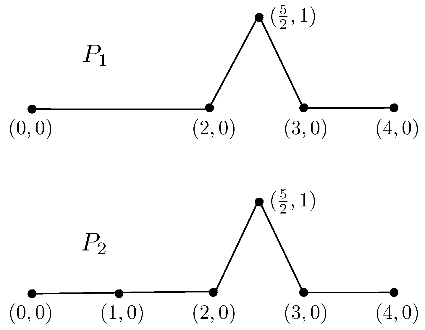
Two polylines are called double-cross similar if their double-cross matrices are identical. Two polylines, that are quite different from a quantitative or metric perspective, may have the same double-cross matrices, as we illustrate below. The idea is that they follow a similar pattern of relative turns, which reflects how humans visualize and remember movement patterns.

In this paper, we provide an extensive algebraic and geometric interpretation of the double-cross matrix of a polyline and of double-cross similarity of polylines. To start with, we give a collection of polynomial constraints (polynomial equalities and inequalities) on the coordinates of the measured points of a polyline (its vertices) that express the information contained in the double-cross matrix of a polyline. This algebraic characterisation can be used to effectively verify double-cross similarity of polylines and to generate double-cross similar polylines by means of tools from algebraic geometry, implemented, for instance, in software packages like Mathematica [31]. This algebraic characterization of the double-cross matrix also allows us to prove a number of properties of double-cross matrices. As an example, we mention a high degree of symmetry in the double-cross matrix along its main diagonal.

Next, we turn to a geometrical interpretation of double-cross similarity of two polylines. This geometrical interpretation is based on local geometric information of the polyline in its vertices. This information is called the local carrier order and it uses (local) compass directions in the vertices of a polyline to locate the relative position of the other vertices. Our main result in this context says that two polylines are double-cross similar if and only if they have the same local carrier order structure.

From the definition of the doubtle-cross matrix of a polyline it is clear that this matrix remains the same if, for instance, we translate or rotate the polyline in the two-dimensional plane. In a final part of this paper, we identify the exact set of transformations of the two-dimensional plane that leave double-cross matrices invariant. Our main (and rather technical) result states that the largest group of transformations of the plane, that is double-cross invariant consist of the similaritiy transformations of the plane onto itself. In broad terms, the similarities of the plane are the translations, rotations and homotecies (scalings) of the plane. This result allows us, for instance, to prove any statement about double-cross matrices of a polyline, only for polylines start in the origin of the two-dimensional plane and have a unit length first line segment.

Organization 

This paper is organized as follows. Section 2 gives the definition of a polyline, the double-cross matrix of a polyline and double-cross similarity of two polylines. It also gives examples of the application of the concept of double-cross similarity in GIS. Section 3 gives our algebraic characterization of the double-cross matrix of a polyline. In Section 4, we derive a number of properties of double-cross matrices from the algebraic characterisation. In Section 5, we give a geometric characterization of the double-cross similarity of two polylines in terms of the local carrier order. And finally, in Section 6, we characterize the double-cross invariant transformations of the plane. In this section, we identify the transformations of the plane that leave the double-cross matrix of all polylines invariant.

2. Definitions and Preliminaries

In this section, we give the definitions of a polyline, of the double-cross matrix of a polyline and of double-cross similarity of two polylines.

2.1. Polylines in the Plane

Let $\mathbf{R}$ denote the set of the real numbers, and let ${\mathbf{R}}^2$ denote the two-dimensional real plane. To stress that some real values are constants, we use sans serif characters: $\mathsf{x},\mathsf{y},{\mathsf{x}}_0,{\mathsf{y}}_0,{\mathsf{x}}_1,{\mathsf{y}}_1,\cdots$. Real variables are denoted in normal characters. For constant points of ${\mathbf{R}}^2$, we use the sans serif characters $\mathsf{p},{\mathsf{p}}_0,{\mathsf{p}}_1,\cdots$

The following definition specifies what we mean by polylines. We define polylines as a finite sequences of points in ${\mathbf{R}}^2$ (which is often used as their finite representation). When we add the line segments between consecutive points we obtain what we call the semantics of the polyline. We also introduce some terminology about polylines.

Definition 1. 

A polyline (in ${\mathbf{R}}^2$) is an ordered list $P=\langle ({\mathsf{x}}_0,{\mathsf{y}}_0),({\mathsf{x}}_1,{\mathsf{y}}_1),,\cdots ,({\mathsf{x}}_N,{\mathsf{y}}_N)\rangle$ of points in ${\mathbf{R}}^2$. We call the points $({\mathsf{x}}_i,{\mathsf{y}}_i)$, $0\le i\le N$, the vertices of the polyline. We assume that no two consecutive vertices are identical, that is: $({\mathsf{x}}_i,{\mathsf{y}}_i)\ne ({\mathsf{x}}_{i+1},{\mathsf{y}}_{i+1})$, for $0\le i<N$.

We call N the size of the polyline P. The vertices $({\mathsf{x}}_0,{\mathsf{y}}_0)$ and $({\mathsf{x}}_N,{\mathsf{y}}_N)$ are respectively called the start and end vertex of P. The line segments connecting the points $({\mathsf{x}}_i,{\mathsf{y}}_i)$ and $({\mathsf{x}}_{i+1},{\mathsf{y}}_{i+1})$, for $0\le i<N$, are called the (line) segments of the polyline P. The semantics of P, denoted $\mathsf{sem}\left(P\right)$, is the union of the line segments of P.

So, the semantics, $\mathsf{sem}\left(P\right)$, is the following union of line segments:

$$\bigcup _{i=0}^{N-1}\left\{(x,y)\in {\mathbf{R}}^2\mid \exists \lambda \in [0,1]:(x,y)=\lambda ·({\mathsf{x}}_i,{\mathsf{y}}_i)+(1-\lambda )·({\mathsf{x}}_{i+1},{\mathsf{y}}_{i+1})\right\},$$

which is a polygonal curve in ${\mathbf{R}}^2$. The quantified real variable λ captures, for values $0<\lambda <1$, the points on the line segments, strictly between the vertices $({\mathsf{x}}_i,{\mathsf{y}}_i)$ and $({\mathsf{x}}_{i+1},{\mathsf{y}}_{i+1})$ in $\mathsf{sem}\left(P\right)$. Further on, we will loosely use the term polyline also to refer to the semantics of a polyline, although, in a strict sense, a polyline is a ordered list of points in ${\mathbf{R}}^2$.

We remark that two polylines with a different number of vertices, may have the same semantics. Figure 1 gives an example of such polylines. We also remark that the line segments, appearing in the semantics, may intersect in points which may or may be not vertices, as is illustrated by the polyline shown in Figure 2. A polyline where the start and end vertex coincide and which has no other self-intersections in its semantics is a polygon. Finally, we remark that it is reasonable to assume that polylines coming from GIS applications have vertices with rational coordinates.

Below, we stick to the notation introduced in the above definitions. Furthermore, as a standard, we abbreviate $({\mathsf{x}}_i,{\mathsf{y}}_i)$ by ${\mathsf{p}}_i$. We also use the following notational conventions. The (located) vector from ${\mathsf{p}}_i$ to ${\mathsf{p}}_j$ is denoted by $\overrightarrow{{\mathsf{p}}_i{\mathsf{p}}_j}$ (by the located vector from $\mathsf{p}$ to $\mathsf{q}$, we mean an ordered pair $(\mathsf{p},\mathsf{q})$ of points of ${\mathbf{R}}^2$). We use this concept to represent the oriented line segment between $\mathsf{p}$ and $\mathsf{q}$. The counter-clockwise angle (expressed in degrees) measured from $\overrightarrow{{\mathsf{p}}_i{\mathsf{p}}_j}$ to $\overrightarrow{{\mathsf{p}}_i{\mathsf{p}}_k}$ is denoted by $\angle (\overrightarrow{{\mathsf{p}}_i{\mathsf{p}}_j},\overrightarrow{{\mathsf{p}}_i{\mathsf{p}}_k})$, as illustrated in Figure 3.

2.2. The Double-Cross Matrix of a Polyline

In this section, we define the double-cross matrix of a polyline.

2.2.1. The Double-Cross Value of Two (Located) Vectors

The double-cross calculus was introduced as a formalism to qualitatively represent a configuration of vectors in the plane ${\mathbf{R}}^2$ [15,26]. In this formalism, the relative position (or orientation) of two (located) vectors is encoded by means of a 4-tuple, whose entries come from the set $\{0,+,-\}$. Such a 4-tuple expresses the relative orientation of two vectors with respect to each other.

We associate to a polyline $P=\langle ({\mathsf{x}}_0,{\mathsf{y}}_0),({\mathsf{x}}_1,{\mathsf{y}}_1),,\cdots ,({\mathsf{x}}_N,{\mathsf{y}}_N)\rangle$, with ${\mathsf{p}}_i=({\mathsf{x}}_i,{\mathsf{y}}_i)$, the (located) vectors $\overrightarrow{{\mathsf{p}}_0{\mathsf{p}}_1},\overrightarrow{{\mathsf{p}}_1{\mathsf{p}}_2},\cdots ,\overrightarrow{{\mathsf{p}}_{N-1}{\mathsf{p}}_N}$, representing the oriented line segments between the consecutive vertices of P. Because of the assumption in Definition 1, the vectors $\overrightarrow{{\mathsf{p}}_0{\mathsf{p}}_1},\overrightarrow{{\mathsf{p}}_1{\mathsf{p}}_2},\cdots ,\overrightarrow{{\mathsf{p}}_{N-1}{\mathsf{p}}_N}$ all have a strictly positive length. In the double-cross formalism, the relative orientation between $\overrightarrow{{\mathsf{p}}_i{\mathsf{p}}_{i+1}}$ and $\overrightarrow{{\mathsf{p}}_j{\mathsf{p}}_{j+1}}$ is given by means of a 4-tuple

$$\left(C_1{C}_2{C}_3{C}_4\right)\in {\{-,0,+\}}^4.$$

We follow the traditional notation of this 4-tuple without commas. To determine $C_1,C_2,C_3$ and $C_4$, for ${\mathsf{p}}_i\ne {\mathsf{p}}_j$, first of all, a double cross is defined for the vectors $\overrightarrow{{\mathsf{p}}_i{\mathsf{p}}_{i+1}}$ and $\overrightarrow{{\mathsf{p}}_j{\mathsf{p}}_{j+1}}$, determined by the following three lines:

• the line $L_{ij}$ through ${\mathsf{p}}_i$ and ${\mathsf{p}}_j$;
• the line $P_{iji}$ through ${\mathsf{p}}_i$, perpendicular on $L_{ij}$; and
• the line $P_{ijj}$ through ${\mathsf{p}}_j$, perpendicular on $L_{ij}$.

These three lines are illustrated in Figure 4. These three lines determine a cross at ${\mathsf{p}}_i$ and a cross at ${\mathsf{p}}_j$. Hence the name “double cross.” The entries $C_1,C_2,C_3$ and $C_4$ express in which quadrants or on which half lines ${\mathsf{p}}_{i+1}$ and ${\mathsf{p}}_{j+1}$ are located with respect to the double cross.

We now define this more formally and follow the historical use of the double cross (see, for instance, [15,26]). In this definition, an interval $(a,b)$ of angles, represents the open interval between a and b on the counter-clockwise oriented circle.

Definition 2. 

Let $P=\langle ({\mathsf{x}}_0,{\mathsf{y}}_0),({\mathsf{x}}_1,{\mathsf{y}}_1),\cdots ,({\mathsf{x}}_N,{\mathsf{y}}_N)\rangle$ be a polyline, with ${\mathsf{p}}_i=({\mathsf{x}}_i,{\mathsf{y}}_i)$, for $0\le i\le N$, and with associated vectors $\overrightarrow{{\mathsf{p}}_0{\mathsf{p}}_1},\overrightarrow{{\mathsf{p}}_1{\mathsf{p}}_2},\cdots ,\overrightarrow{{\mathsf{p}}_{N-1}{\mathsf{p}}_N}$. For $\overrightarrow{{\mathsf{p}}_i{\mathsf{p}}_{i+1}}$ and $\overrightarrow{{\mathsf{p}}_j{\mathsf{p}}_{j+1}}$ with $0\le i,j<N$, $i\ne j$ and ${\mathsf{p}}_i\ne {\mathsf{p}}_j$, we define

$$\mathsf{DC}(\overrightarrow{{\mathsf{p}}_i{\mathsf{p}}_{i+1}},\overrightarrow{{\mathsf{p}}_j{\mathsf{p}}_{j+1}})=\left(C_1{C}_2{C}_3{C}_4\right)$$

as follows:

$C_1$	=	$\left\{\begin{array}{ccc}-\hfill & if\hfill & \angle (\overrightarrow{{\mathsf{p}}_i{\mathsf{p}}_j},\overrightarrow{{\mathsf{p}}_i{\mathsf{p}}_{i+1}})\in (-{90}^{\circ },{90}^{\circ })\hfill \\ 0\hfill & if\hfill & \angle (\overrightarrow{{\mathsf{p}}_i{\mathsf{p}}_j},\overrightarrow{{\mathsf{p}}_i{\mathsf{p}}_{i+1}})\in \{-{90}^{\circ },{90}^{\circ }\}\hfill \\ +\hfill & else\hfill & \end{array}\right.$
$C_2$	=	$\left\{\begin{array}{ccc}-\hfill & if\hfill & \angle (\overrightarrow{{\mathsf{p}}_j{\mathsf{p}}_i},\overrightarrow{{\mathsf{p}}_j{\mathsf{p}}_{j+1}})\in (-{90}^{\circ },{90}^{\circ })\hfill \\ 0\hfill & if\hfill & \angle (\overrightarrow{{\mathsf{p}}_j{\mathsf{p}}_i},\overrightarrow{{\mathsf{p}}_j{\mathsf{p}}_{j+1}})\in \{-{90}^{\circ },{90}^{\circ }\}\hfill \\ +\hfill & else\hfill & \end{array}\right.$
$C_3$	=	$\left\{\begin{array}{ccc}-\hfill & if\hfill & \angle (\overrightarrow{{\mathsf{p}}_i{\mathsf{p}}_j},\overrightarrow{{\mathsf{p}}_i{\mathsf{p}}_{i+1}})\in (0^{\circ },{180}^{\circ })\hfill \\ 0\hfill & if\hfill & \angle (\overrightarrow{{\mathsf{p}}_i{\mathsf{p}}_j},\overrightarrow{{\mathsf{p}}_i{\mathsf{p}}_{i+1}})\in \{0^{\circ },{180}^{\circ }\}\hfill \\ +\hfill & else\hfill & \end{array}\right.$
$C_4$	=	$\left\{\begin{array}{ccc}-\hfill & if\hfill & \angle (\overrightarrow{{\mathsf{p}}_j{\mathsf{p}}_i},\overrightarrow{{\mathsf{p}}_j{\mathsf{p}}_{j+1}})\in (0^{\circ },{180}^{\circ })\hfill \\ 0\hfill & if\hfill & \angle (\overrightarrow{{\mathsf{p}}_j{\mathsf{p}}_i},\overrightarrow{{\mathsf{p}}_j{\mathsf{p}}_{j+1}})\in \{0^{\circ },{180}^{\circ }\}\hfill \\ +\hfill & else.\hfill & \end{array}\right.$

For $\overrightarrow{{\mathsf{p}}_i{\mathsf{p}}_{i+1}}$ and $\overrightarrow{{\mathsf{p}}_j{\mathsf{p}}_{j+1}}$, with ${\mathsf{p}}_i={\mathsf{p}}_j$, we define, for reasons of continuity,

$$\mathsf{DC}(\overrightarrow{{\mathsf{p}}_i{\mathsf{p}}_{i+1}},\overrightarrow{{\mathsf{p}}_j{\mathsf{p}}_{j+1}})=\left(0000\right).$$

The argumentation for this convention is given in [32].

So, in particular, when $i=j$, we have $\mathsf{DC}(\overrightarrow{{\mathsf{p}}_i{\mathsf{p}}_{i+1}},\overrightarrow{{\mathsf{p}}_j{\mathsf{p}}_{j+1}})=\left(0000\right)$.

We remark that the values $C_1$ and $C_3$ describe the location of the point ${\mathsf{p}}_{i+1}$ or, equivalently, the orientation of the vector $\overrightarrow{{\mathsf{p}}_i{\mathsf{p}}_{i+1}}$ with respect to the cross at ${\mathsf{p}}_i$ (formed by the lines $L_{ij}$ and $P_{iji}$). We see that each of the four quadrants and four half lines determined by the cross at ${\mathsf{p}}_i$ are determined by a unique combination of $C_1$ and $C_3$ values. Similarly, the values $C_2$ and $C_4$ describe the location of the point ${\mathsf{p}}_{j+1}$ or, equivalently, the orientation of the vector $\overrightarrow{{\mathsf{p}}_j{\mathsf{p}}_{j+1}}$ with respect to the cross at ${\mathsf{p}}_j$ (formed by the lines $L_{ij}$ and $P_{ijj}$).

The quadrants and half lines where $C_1$, $C_2$, $C_3$ and $C_4$ take different values are graphically illustrated in Figure 5. For example, the 4-tuple $\mathsf{DC}(\overrightarrow{{\mathsf{p}}_i{\mathsf{p}}_{i+1}},\overrightarrow{{\mathsf{p}}_j{\mathsf{p}}_{j+1}})$ for the vectors $\overrightarrow{{\mathsf{p}}_i{\mathsf{p}}_{i+1}}$ and $\overrightarrow{{\mathsf{p}}_j{\mathsf{p}}_{j+1}}$, shown in Figure 4, is $(+---)$.

Further on, we will sometimes use the notation $\mathsf{DC}(\overrightarrow{{\mathsf{p}}_i{\mathsf{p}}_{i+1}},\overrightarrow{{\mathsf{p}}_j{\mathsf{p}}_{j+1}})\left[k\right]$ to indicate $C_k$, for $k=1,2,3,4$. Obviously, this notation does not hide the dependence on i and j.

Remark. 

Since $C_1$, $C_2$, $C_3$ and $C_4$ take values from the set $\{-,0,+\}$, it may seem that there are $3^4=81$ possible values for the tuples $\left(C_1{C}_2{C}_3{C}_4\right)$.

However, some combinations are not possible because of the assumption in Definition 1, that says that two consecutive vertices of a polyline have to be different. This means that $C_1$ and $C_3$ cannot be both 0 and that $C_2$ and $C_4$ cannot be both 0, in each case with the exception of $C_1$, $C_2$, $C_3$ and $C_4$ all being 0, that is $\left(C_1{C}_2{C}_3{C}_4\right)=\left(0000\right)$. So, we have $81-8-8=65$ possible values for $\left(C_1{C}_2{C}_3{C}_4\right)$.

This number of 65 possible values for the tuples $\left(C_1{C}_2{C}_3{C}_4\right)$ can also be reached in another way. The point ${\mathsf{p}}_{i+1}$ can be in one of four quadrants around ${\mathsf{p}}_i$ or on one of four half lines starting in ${\mathsf{p}}_i$. These are 8 possible locations for ${\mathsf{p}}_{i+1}$. Similarly, we have 8 possible locations for ${\mathsf{p}}_{j+1}$ in the quadrants and half lines starting in ${\mathsf{p}}_j$. This gives $8\times 8=64$ possible combinations. Together with the case $\left(C_1{C}_2{C}_3{C}_4\right)=\left(0000\right)$, we reach a total number of 65 possibilities.

2.2.2. The Double-Cross Matrix of a Polyline

Based on the definition of $\mathsf{DC}(\overrightarrow{{\mathsf{p}}_i{\mathsf{p}}_{i+1}},\overrightarrow{{\mathsf{p}}_j{\mathsf{p}}_{j+1}})$, we now define the double-cross matrix of a polyline.

Definition 3. 

Let $P=\langle ({\mathsf{x}}_0,{\mathsf{y}}_0),({\mathsf{x}}_1,{\mathsf{y}}_1),\cdots ,({\mathsf{x}}_N,{\mathsf{y}}_N)\rangle$ be a polyline, with ${\mathsf{p}}_i=({\mathsf{x}}_i,{\mathsf{y}}_i)$, for $0\le i\le N$, and with associated vectors $\overrightarrow{{\mathsf{p}}_0{\mathsf{p}}_1},\overrightarrow{{\mathsf{p}}_1{\mathsf{p}}_2},\cdots ,\overrightarrow{{\mathsf{p}}_{N-1}{\mathsf{p}}_N}$. The double-cross matrix of P, denoted $\mathsf{DCM}\left(P\right)$, is the $N\times N$ matrix with the entries $\mathsf{DCM}\left(P\right)[i,j]=\mathsf{DC}(\overrightarrow{p_i{p}_{i+1}},\overrightarrow{p_j{p}_{j+1}})$, for $0\le i,j<N$.

For example, the entries of the double-cross matrix of the polyline of Figure 6 are given in

Table 1. The entries of the double-cross matrix of the polyline of Figure 6.

	$\overrightarrow{{\mathsf{p}}_0{\mathsf{p}}_1}$	$\overrightarrow{{\mathsf{p}}_1{\mathsf{p}}_2}$	$\overrightarrow{{\mathsf{p}}_2{\mathsf{p}}_3}$	$\overrightarrow{{\mathsf{p}}_3{\mathsf{p}}_4}$	$\overrightarrow{{\mathsf{p}}_4{\mathsf{p}}_5}$
$\overrightarrow{{\mathsf{p}}_0{\mathsf{p}}_1}$	$\left(0000\right)$	$(--0+)$	$(-++-)$	$(--+-)$	$(-+-+)$
$\overrightarrow{{\mathsf{p}}_1{\mathsf{p}}_2}$	$(--+0)$	$\left(0000\right)$	$(--0+)$	$(-+++)$	$(--++)$
$\overrightarrow{{\mathsf{p}}_2{\mathsf{p}}_3}$	$(---+)$	$(--+0)$	$\left(0000\right)$	$(-+0-)$	$(---+)$
$\overrightarrow{{\mathsf{p}}_3{\mathsf{p}}_4}$	$(---+)$	$(+-++)$	$(+--0)$	$\left(0000\right)$	$(--0+)$
$\overrightarrow{{\mathsf{p}}_4{\mathsf{p}}_5}$	$(+-+-)$	$(--++)$	$(--+-)$	$(--+0)$	$\left(0000\right)$

. This first example can be used to illustrate some properties of this matrix that are proven in Section 4. First, we observe that on the diagonal always $\left(0000\right)$ appears. We also see that there is a certain degree of symmetry along the diagonal. If $\mathsf{DC}(\overrightarrow{{\mathsf{p}}_i{\mathsf{p}}_{i+1}},\overrightarrow{{\mathsf{p}}_j{\mathsf{p}}_{j+1}})=\left(C_1{C}_2{C}_3{C}_4\right)$, then we have $\mathsf{DC}(\overrightarrow{{\mathsf{p}}_j{\mathsf{p}}_{j+1}},\overrightarrow{{\mathsf{p}}_i{\mathsf{p}}_{i+1}})=\left(C_2{C}_1{C}_4{C}_3\right)$. These two observations imply that it suffices to know a double-cross matrix above its diagonal.

2.3. Double-Cross Similarity of Polylines

We now define double-cross similarity of two polylines of equal size.

Definition 4. 

Let P and Q be polylines of the same size. We say that P and Q are double-cross similar if $\mathsf{DCM}\left(P\right)=\mathsf{DCM}\left(Q\right)$.

We stress that Definition 4 requires that the two polylines have to be of the same size before we can speak of their double-cross similarity.

Figure 7 depicts two polylines, P and Q, which are double-cross similar. The entries of their double-cross matrices are given in

Table 2. The entries of the double-cross matrix of the polylines of Figure 7.

	$\overrightarrow{{\mathsf{p}}_0{\mathsf{p}}_1}$	$\overrightarrow{{\mathsf{p}}_1{\mathsf{p}}_2}$	$\overrightarrow{{\mathsf{p}}_2{\mathsf{p}}_3}$	$\overrightarrow{{\mathsf{p}}_3{\mathsf{p}}_4}$	$\overrightarrow{{\mathsf{p}}_4{\mathsf{p}}_5}$
$\overrightarrow{{\mathsf{p}}_0{\mathsf{p}}_1}$	$\left(0000\right)$	$(-+0+)$	$(-+++)$	$(-+++)$	$(-+++)$
$\overrightarrow{{\mathsf{p}}_1{\mathsf{p}}_2}$	$(+-+0)$	$\left(0000\right)$	$(-+0+)$	$(-+++)$	$(-+++)$
$\overrightarrow{{\mathsf{p}}_2{\mathsf{p}}_3}$	$(+-++)$	$(+-+0)$	$\left(0000\right)$	$(-+0+)$	$(-+++)$
$\overrightarrow{{\mathsf{p}}_3{\mathsf{p}}_4}$	$(+-++)$	$(+-++)$	$(+-+0)$	$\left(0000\right)$	$(-+0+)$
$\overrightarrow{{\mathsf{p}}_4{\mathsf{p}}_5}$	$(+-++)$	$(+-++)$	$(+-++)$	$(+-+0)$	$\left(0000\right)$

. In polyline P of Figure 7, at each vertex, the polyline bends around 10 degrees to the left. In polyline Q, this is only around 2 degrees. Nevertheless, all relative positions of oriented line segments remain the same. As the most extreme example, if we compare $\overrightarrow{{\mathsf{p}}_0{\mathsf{p}}_1}$ and $\overrightarrow{{\mathsf{p}}_4{\mathsf{p}}_5}$ in both polylines, we see that $\overrightarrow{{\mathsf{p}}_4{\mathsf{p}}_5}$ almost makes a ${90}^{\circ }$ left angle with the central line of the double cross in the polyline P, whereas, this is only some ${10}^{\circ }$ in the polyline Q. Still, both P and Q have the same double-cross entry for $\overrightarrow{{\mathsf{p}}_0{\mathsf{p}}_1}$ and $\overrightarrow{{\mathsf{p}}_4{\mathsf{p}}_5}$.

2.4. Examples of The Application of Double-Cross Similarity in GIS

In this section, we give some examples of the applicability of the concept of double-cross similarity of polylines in the area of GIS [27]. Polyline- (and polygon-) similarity testing, based on the double-cross formalism, can be applied in a number of areas in GIS. We think of applications in the area of image recognition or retrieval in the context of geographical maps. Features in maps are often modelled as polylines (for instance, roads and rivers) and polygons (for example, closed polylines can be used to delimit geographical areas such as cities, provinces and countries). Polyline-similarity testing can also be applied in the area of the classification of terrain features. In spatial database terms, it can be used for querying-by-sketch.

To determine the degree of similarity between two polylines (not necessary of the same size), according to the double-cross formalism, we can proceed by the following two steps: (1) first, if the polylines are of different size, their “generalized polylines” (that approximate the original polylines within an ε-error margin) are computed; (2) next, the differences between the double-cross matrices of the generalized polylines are used as a measure of dissimilarity between the given polylines. In the remainder of this section, we describe this process in some more detail and we give some examples of its application.

The definition of double-cross similarity of polylines (Definition 4) can only be applied to polylines of the same size. Obviously, in practice, we often want to test similarity of polylines that are not necessarily of the same size. To overcome this problem, we can use the notion of “generalized polylines”: for a given polyline P, a sequence of generalized polylines $P^2,P^4,P^8,\dots ,P^{2^n},\dots$ are defined that tend (as n grows) to converge to P (arbitrary close) and to consist of equally long line segments. To define the generalized polyline $P^{2^n}$ in this sequence, we measure the distance along P from its start vertex to its end vertex and we mark on $\mathsf{sem}\left(P\right)$ the $2^n+1$ points that divide $\mathsf{sem}\left(P\right)$ in pieces of equal length. These markers are used as the $2^n+1$ vertices of the generalized polyline $P^{2^n}$. The first generalizations $P^2$, $P^4$ and $P^8$ of a polyline P are shown in Figure 8. It can be shown that the generalized polylines of P converge to P, as n grows. This means that, for any error margin $\epsilon >0$, a polyline P can be approximated, for sufficiently large n, by its generalizations $P^{2^n}$ up to an error of ε. In particular, the difference in length between P and $P^{2^n}$ is less than ε [27].

This means that for two given polylines $P_1$ and $P_2$ and an arbitrarily small ε, we can find a large enough n such that both $P_1^{2^n}$ and $P_2^{2^n}$ are ε-close to $P_1$ and $P_2$. For step (2), we can use the double-cross matrices $M_1$ and $M_2$ of $P_1^{2^n}$ and $P_2^{2^n}$ to define the double-cross (dis)similarity of $P_1$ and $P_2$. There are many possibilities here, but in the experiments in [27], the distance function ${\Delta }_H$ is shown to be the most suitable in many applications in GIS. To define the distance measure ${\Delta }_H(M_1,M_2)$ between double-cross matrices, we first construct, for both matrices $M_1$ and $M_2$, 65-ary vectors $\gamma \left(M_1\right),\gamma \left(M_2\right)$ over the natural numbers, that count for each of the 65 realizable 4-tuples of −, + and 0 (Proposition 10 explains the number 65), the number of times they occur in the matrices $M_1$ and $M_2$. Then, for matrices $M_1$ and $M_2$ of polylines of size N, we define

$${\Delta }_H(M_1,M_2):=\frac{1}{N^2-N}\sum _{i=1}^{65}\left|\gamma \left(M_1\right)\left[i\right]-\gamma \left(M_2\right)\left[i\right]\right|,$$

where $N=2^n$ and where $\gamma \left(M_1\right)\left[i\right]$ refers to the ith entry of the vector $\gamma \left(M_1\right)$. This means that the function ${\Delta }_H$ counts the average difference between the 65 count values. In [27], it is shown that ${\Delta }_H$ can be efficiently computed. It was also shown to perform well in a number of applications. We conclude this section, by discussing some of the performance results of ${\Delta }_H$.

Example 1: Polygon Similarity: Image Recognition and the Classification of Terrain Features

Figure 9 shows a map of Belgium in Figure 9a, consisting of 2047 line segments. Figure 9b is the same figure with the three bumps in the upper part moved to the right. Figure 9c is a map drawn by a geographer and Figure 9d is an abstract representation.

Table 3. Similarity between polygons of Figure 9 using ${\Delta }_H$.

Figure	(a)	(b)	(c)	(d)
(a)	100%	99%	87%	66%
(b)		100%	87%	67%
(c)			100%	80%
(d)				100%

gives an overview of the similarity levels determined by ${\Delta }_H$. For example, the actual map of Belgium is 99% similar to the slightly modified map, but only 60% similar to the abstract representation.

This technique of ${\Delta }_H$-based polygon similarity can be used in areas such as image retrievel or recognition, but also in the recognition and classification of terrain features, of which the basic terrain features, modelled as polylines, are depicted in Figure 10.

Example 2: Query-by-Sketch

Figure 11 first shows sketches of a bowler hat and a bow tie. Next, it shows a map of the the province of Limburg in Belgium with its municipalities. The municipalities that resemble the bowler hat the most, according to ${\Delta }_H$, are shown in black on this map. The most alike city is “Lommel”, as indicated in the figure. The municipalities, resembling the bow tie sketch, are shown in grey.

For further implementation details and experimental results, we refer to [27].

3. An Algebraic Characterization of the Double-Cross Aatrix of a Polyline

In this section, we give an algebraic characterization of the entries in the double-cross matrix of a polyline. This algebraic characterisation can be used to effectively verify double-cross similarity of polylines.

Let $P=\langle ({\mathsf{x}}_0,{\mathsf{y}}_0),({\mathsf{x}}_1,{\mathsf{y}}_1),\cdots ,({\mathsf{x}}_N,{\mathsf{y}}_N)\rangle$ be a polyline and let ${\mathsf{p}}_i=({\mathsf{x}}_i,{\mathsf{y}}_i)$, for $0\le i\le N$. Theorem 5 gives algebraic expressions to calculate the entries $\mathsf{DC}(\overrightarrow{{\mathsf{p}}_i{\mathsf{p}}_{i+1}},\overrightarrow{{\mathsf{p}}_j{\mathsf{p}}_{j+1}})$ of a double-cross matrix in terms of the x- and y-coordinates of the points ${\mathsf{p}}_i,{\mathsf{p}}_{i+1},{\mathsf{p}}_j$ and ${\mathsf{p}}_{j+1}$. Further on, we use this theorem extensively to prove properties of double-cross matrices.

Before stating and proving this theorem, we recall some elementary notations from algebra and some formula’s in the following remark.

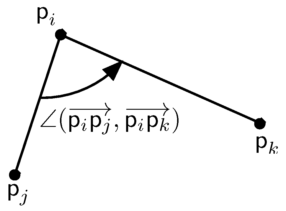
Remark. 

The well-known formula to calculate the (counter-clockwise) angle θ between two vectors $\overrightarrow{a}$ and $\overrightarrow{b}$ in ${\mathbf{R}}^2$ (and also, in general, in ${\mathbf{R}}^n$) is

$$cos\theta =\frac{\overrightarrow{a}·\overrightarrow{b}}{|\overrightarrow{a}|·|\overrightarrow{b}|}.$$

Here, we are not talking about located vectors like before, but vectors in the common sense. In the above formula, the · in the numerator denotes the inner product (also called scalar product) of two vectors and $|\overrightarrow{a}|$ is the norm or length of $\overrightarrow{a}$ (and the · in the denominator is the product of real numbers).

The above formula implies that we have $cos\theta =0$ if and only if $\overrightarrow{a}·\overrightarrow{b}=0$ if and only if $\theta \in \{{90}^{\circ },-{90}^{\circ }\}$. So, $\overrightarrow{a}·\overrightarrow{b}=0$ means that $\overrightarrow{a}$ is perpendicular to $\overrightarrow{b}$. On the other hand, we have $cos\theta >0$ and thus $\overrightarrow{a}·\overrightarrow{b}>0$, when $\theta \in (-{90}^{\circ },{90}^{\circ })$. And finally $\overrightarrow{a}·\overrightarrow{b}<0$ is equivalent to $\theta \in ({90}^{\circ },{270}^{\circ })$.

If $\overrightarrow{a}=(a,b)\in {\mathbf{R}}^2$, then ${\overrightarrow{a}}^{\perp }=(-b,a)$ is the unique vector, perpendicular to $\overrightarrow{a}$ and of the same length of $\overrightarrow{a}$, such that the (counter-clockwise) angle from $\overrightarrow{a}$ to ${\overrightarrow{a}}^{\perp }$ is ${90}^{\circ }$.

In the following theorem, we use the function

$$\mathrm{sign}:\mathbf{R}\to \{-,0,+\}:x\mapsto sign\left(x\right)=\left\{\begin{array}{ccc}-& if\hfill & x<0;\hfill \\ 0& if\hfill & x=0;and\hfill \\ +& if\hfill & x>0.\hfill \end{array}\right.$$

We also work with the following convention concerning signs: $--$ is +; $-0$ is 0; and $-+$ is −.

Theorem 5. 

Let $P=\langle ({\mathsf{x}}_0,{\mathsf{y}}_0),({\mathsf{x}}_1,{\mathsf{y}}_1),\cdots ,({\mathsf{x}}_N,{\mathsf{y}}_N)\rangle$ be a polyline and let ${\mathsf{p}}_i=({\mathsf{x}}_i,{\mathsf{y}}_i)$, for $0\le i\le N$. Then, $\mathsf{DC}(\overrightarrow{{\mathsf{p}}_i{\mathsf{p}}_{i+1}},\overrightarrow{{\mathsf{p}}_j{\mathsf{p}}_{j+1}})=\left(C_1{C}_2{C}_3{C}_4\right)$ with

$C_1$	=	−	$\mathrm{sign}(({\mathsf{x}}_j-{\mathsf{x}}_i)·({\mathsf{x}}_{i+1}-{\mathsf{x}}_i)+({\mathsf{y}}_j-{\mathsf{y}}_i)·({\mathsf{y}}_{i+1}-{\mathsf{y}}_i));$
$C_2$	=		$\mathrm{sign}(({\mathsf{x}}_j-{\mathsf{x}}_i)·({\mathsf{x}}_{j+1}-{\mathsf{x}}_j)+({\mathsf{y}}_j-{\mathsf{y}}_i)·({\mathsf{y}}_{j+1}-{\mathsf{y}}_j));$
$C_3$	=	−	$\mathrm{sign}(({\mathsf{x}}_j-{\mathsf{x}}_i)·({\mathsf{y}}_{i+1}-{\mathsf{y}}_i)-({\mathsf{y}}_j-{\mathsf{y}}_i)·({\mathsf{x}}_{i+1}-{\mathsf{x}}_i))$; and
$C_4$	=		$\mathrm{sign}(({\mathsf{x}}_j-{\mathsf{x}}_i)·({\mathsf{y}}_{j+1}-{\mathsf{y}}_j)-({\mathsf{y}}_j-{\mathsf{y}}_i)·({\mathsf{x}}_{j+1}-{\mathsf{x}}_j))$.

Proof. 

We have ${\mathsf{p}}_i={\mathsf{p}}_j$ if and only if ${\mathsf{x}}_j-{\mathsf{x}}_i=0$ and ${\mathsf{y}}_j-{\mathsf{y}}_i=0$ and in this case the four (instantiated) polynomials in the statement of the theorem evaluate to zero.

Next, we assume ${\mathsf{p}}_i\ne {\mathsf{p}}_j$. We consider the following vectors in ${\mathbf{R}}^2$:

• $\overrightarrow{u_{ij}}=({\mathsf{x}}_j-{\mathsf{x}}_i,{\mathsf{y}}_j-{\mathsf{y}}_i)$;
• $\overrightarrow{u_{ji}}=({\mathsf{x}}_i-{\mathsf{x}}_j,{\mathsf{y}}_i-{\mathsf{y}}_j)$;
• $\overrightarrow{v_i}=({\mathsf{x}}_{i+1}-{\mathsf{x}}_i,{\mathsf{y}}_{i+1}-{\mathsf{y}}_i)$; and
• $\overrightarrow{v_j}=({\mathsf{x}}_{j+1}-{\mathsf{x}}_j,{\mathsf{y}}_{j+1}-{\mathsf{y}}_j)$.

We remark that $\overrightarrow{u_{ij}}=-\overrightarrow{u_{ji}}$ and that the vectors $\overrightarrow{u_{ij}}$, $\overrightarrow{v_i}$ and $\overrightarrow{v_j}$ (in the common sense of the word vector) are the (located) vectors $\overrightarrow{{\mathsf{p}}_i{\mathsf{p}}_j}$, $\overrightarrow{{\mathsf{p}}_i{\mathsf{p}}_{i+1}}$ and $\overrightarrow{{\mathsf{p}}_j{\mathsf{p}}_{j+1}}$ translated to the origin of ${\mathbf{R}}^2$.

• $C_1$: Now, we apply the above cosine-formula to $\overrightarrow{a}=\overrightarrow{u_{ij}}$ and $\overrightarrow{b}=\overrightarrow{v_i}$ to obtain an expression for $C_1$. Because $C_1$ is negative towards ${\mathsf{p}}_j$, we get the minus-sign in the following expression for $C_1$:

$C_1$	=	$-\mathrm{sign}(\overrightarrow{u_{ij}}·\overrightarrow{v_i})$
	=	$-\mathrm{sign}(({\mathsf{x}}_j-{\mathsf{x}}_i)·({\mathsf{x}}_{i+1}-{\mathsf{x}}_i)+({\mathsf{y}}_j-{\mathsf{y}}_i)·({\mathsf{y}}_{i+1}-{\mathsf{y}}_i))$.

• $C_2$: Next, we apply the cosine-formula to $\overrightarrow{a}=\overrightarrow{u_{ji}}$ and $\overrightarrow{b}=\overrightarrow{v_j}$ to obtain an expression for $C_2$. Again, because $C_2$ is negative towards ${\mathsf{p}}_i$, we get the minus-sign in $C_2=-\mathrm{sign}(\overrightarrow{u_{ji}}·\overrightarrow{v_j})$. This means that

$C_2$	=	$\mathrm{sign}(\overrightarrow{u_{ij}}·\overrightarrow{v_j})$
	=	$\mathrm{sign}(({\mathsf{x}}_j-{\mathsf{x}}_i)·({\mathsf{x}}_{j+1}-{\mathsf{x}}_j)+({\mathsf{y}}_j-{\mathsf{y}}_i)·({\mathsf{y}}_{j+1}-{\mathsf{y}}_j))$.

• $C_3$: Here, we apply the cosine-formula to $\overrightarrow{a}={\overrightarrow{u_{ij}}}^{\perp }$ and $\overrightarrow{b}=\overrightarrow{v_i}$ and get $C_3=-\mathrm{sign}({\overrightarrow{u_{ij}}}^{\perp }·\overrightarrow{v_i})$. We have a minus-sign here, because $C_3=-$ in the direction of ${\overrightarrow{u_{ij}}}^{\perp }$. Since ${\overrightarrow{u_{ij}}}^{\perp }=(-({\mathsf{y}}_j-{\mathsf{y}}_i),{\mathsf{x}}_j-{\mathsf{x}}_i)$, we get

$C_3$	=	$-\mathrm{sign}({\overrightarrow{u_{ij}}}^{\perp }·\overrightarrow{v_i})$
	=	$\mathrm{sign}(({\mathsf{y}}_j-{\mathsf{y}}_i)·({\mathsf{x}}_{i+1}-{\mathsf{x}}_i)-({\mathsf{x}}_j-{\mathsf{x}}_i)·({\mathsf{y}}_{i+1}-{\mathsf{y}}_i))$.

• $C_4$: Finally, we apply the cosine-formula to $\overrightarrow{a}={\overrightarrow{u_{ji}}}^{\perp }$ and $\overrightarrow{b}=\overrightarrow{v_j}$. Since $C_4=-$ in the direction of ${\overrightarrow{u_{ji}}}^{\perp }$, we have $C_4=-\mathrm{sign}({\overrightarrow{u_{ji}}}^{\perp }·\overrightarrow{v_j})$. Since ${\overrightarrow{u_{ji}}}^{\perp }=({\mathsf{y}}_j-{\mathsf{y}}_i,-({\mathsf{x}}_j-{\mathsf{x}}_i))$, we get

$C_4$	=	$-\mathrm{sign}({\overrightarrow{u_{ji}}}^{\perp }·\overrightarrow{v_j})$
	=	$\mathrm{sign}(-({\mathsf{y}}_j-{\mathsf{y}}_i)·({\mathsf{x}}_{j+1}-{\mathsf{x}}_j)+({\mathsf{x}}_j-{\mathsf{x}}_i)·({\mathsf{y}}_{i+1}-{\mathsf{y}}_i))$.

This concludes the proof.

In the following property, we show that the double-cross value $\left(0000\right)$, which, for reasons of continuity, is the value in the case ${\mathsf{p}}_i={\mathsf{p}}_j$ (see Definition 2), can only occur in that exceptional case.

Proposition 6. 

Let $P=\langle ({\mathsf{x}}_0,{\mathsf{y}}_0),({\mathsf{x}}_1,{\mathsf{y}}_1),\cdots ,({\mathsf{x}}_N,{\mathsf{y}}_N)\rangle$ be a polyline and let ${\mathsf{p}}_i=({\mathsf{x}}_i,{\mathsf{y}}_i)$. Then, $\mathsf{DC}(\overrightarrow{{\mathsf{p}}_i{\mathsf{p}}_{i+1}},\overrightarrow{{\mathsf{p}}_j{\mathsf{p}}_{j+1}})=\left(0000\right)$ if and only if ${\mathsf{p}}_i={\mathsf{p}}_j$.

Proof. 

As already observed in the proof of Theorem 5, ${\mathsf{p}}_i={\mathsf{p}}_j$ implies ${\mathsf{x}}_j-{\mathsf{x}}_i=0$ and ${\mathsf{y}}_j-{\mathsf{y}}_i=0$ and in this case the four (instantiated) polynomials of Theorem 5 evaluate to zero. This implies that $\mathsf{DC}(\overrightarrow{{\mathsf{p}}_i{\mathsf{p}}_{i+1}},\overrightarrow{{\mathsf{p}}_j{\mathsf{p}}_{j+1}})=\left(0000\right)$.

For the converse, we have to show that if the four polynomials evaluate to zero, then ${\mathsf{p}}_i={\mathsf{p}}_j$. We prove this by assuming ${\mathsf{p}}_i\ne {\mathsf{p}}_j$ and deriving a contradiction. If ${\mathsf{p}}_i\ne {\mathsf{p}}_j$, then ${\mathsf{x}}_j-{\mathsf{x}}_i\ne 0$ or ${\mathsf{y}}_j-{\mathsf{y}}_i\ne 0$. First, we consider the case ${\mathsf{x}}_j-{\mathsf{x}}_i\ne 0$.

As a first subcase, we consider the case ${\mathsf{y}}_j-{\mathsf{y}}_i=0$. Then we get from the equations $C_1=0$ and $C_3=0$ that $({\mathsf{x}}_j-{\mathsf{x}}_i)·({\mathsf{x}}_{i+1}-{\mathsf{x}}_i)=0$ and $({\mathsf{x}}_j-{\mathsf{x}}_i)·({\mathsf{y}}_{i+1}-{\mathsf{y}}_i)=0$. Since ${\mathsf{x}}_j-{\mathsf{x}}_i\ne 0$ is assumed, this implies that ${\mathsf{x}}_{i+1}-{\mathsf{x}}_i=0$ and ${\mathsf{y}}_{i+1}-{\mathsf{y}}_i=0$. This contradicts the assumption in Definition 1, which says that no two consecutive vertices of a polyline are identical.

As a second subcase, we consider the case ${\mathsf{y}}_j-{\mathsf{y}}_i\ne 0$. Then we get from $C_1=0$ that

$${\mathsf{x}}_{i+1}-{\mathsf{x}}_i=\frac{-({\mathsf{y}}_j-{\mathsf{y}}_i)·({\mathsf{y}}_{i+1}-{\mathsf{y}}_i)}{{\mathsf{x}}_j-{\mathsf{x}}_i}$$

From $C_3=0$, we get $({\mathsf{x}}_j-{\mathsf{x}}_i)·({\mathsf{y}}_{i+1}-{\mathsf{y}}_i)=({\mathsf{y}}_j-{\mathsf{y}}_i)·({\mathsf{x}}_{i+1}-{\mathsf{x}}_i).$

Combined, these two equalities imply $({({\mathsf{x}}_j-{\mathsf{x}}_i)}^2+{({\mathsf{y}}_j-{\mathsf{y}}_i)}^2)·({\mathsf{y}}_{i+1}-{\mathsf{y}}_i)=0.$ Since in this case ${({\mathsf{x}}_j-{\mathsf{x}}_i)}^2+{({\mathsf{y}}_j-{\mathsf{y}}_i)}^2>0$, we conclude ${\mathsf{y}}_{i+1}-{\mathsf{y}}_i=0$. But then, again using the equation for $C_1$, we get $({\mathsf{x}}_j-{\mathsf{x}}_i)·({\mathsf{x}}_{i+1}-{\mathsf{x}}_i)=0$, or ${\mathsf{x}}_{i+1}-{\mathsf{x}}_i=0$. So, we have both ${\mathsf{x}}_{i+1}-{\mathsf{x}}_i=0$ and ${\mathsf{y}}_{i+1}-{\mathsf{y}}_i=0$, which again contradicts the assumption in Definition 1. We have contradiction in all cases and this concludes the proof of the first case. The case ${\mathsf{y}}_j-{\mathsf{y}}_i\ne 0$ has a completely analogous proof, now using $C_2=0$ and $C_4=0$ instead of $C_1=0$ and $C_3=0.$ This concludes the proof.

We end this section by remarking that all the factors appearing in the algebraic expressions, given by the theorem, that is ${\mathsf{x}}_j-{\mathsf{x}}_i$, ${\mathsf{x}}_{i+1}-{\mathsf{x}}_i$, ${\mathsf{y}}_j-{\mathsf{y}}_i$, ${\mathsf{y}}_{i+1}-{\mathsf{y}}_i$, ${\mathsf{x}}_{j+1}-{\mathsf{x}}_j$ and ${\mathsf{y}}_{j+1}-{\mathsf{y}}_j$ are differences in x-coordinate or differences in y-coordinate values.

4. Some Properties of Double-Cross Matrices that can be Derived from Their Algebraic Characterisation

In this section, we give some basic properties of double-cross matrices of polylines. In most cases, these properties can be derived from the algebraic characterization of the entries of a double-cross matrix, that we presented in previous section.

4.1. Symmetry in the Double-Cross Matrix of a Polyline

In Section 2.2.2, we have already announced by the example polyline given in Figure 6 with its double-cross matrix given in Table 1, that a double-cross matrix exhibits symmetry properties. We prove these properties in this section. The first property is by definition, the second needs some inspection of polynomials. The conclusion is that it is enough to know a double-cross matrix above its diagonal.

Proposition 7. 

If $P=\langle {\mathsf{p}}_0,{\mathsf{p}}_1,\cdots ,{\mathsf{p}}_N\rangle$ is a polyline, then $\mathsf{DC}(\overrightarrow{{\mathsf{p}}_i{\mathsf{p}}_{i+1}},\overrightarrow{{\mathsf{p}}_i{\mathsf{p}}_{i+1}})=\left(0000\right)$, for $0\le i<N$.

The following property says how $\mathsf{DC}(\overrightarrow{{\mathsf{p}}_j{\mathsf{p}}_{j+1}},\overrightarrow{{\mathsf{p}}_i{\mathsf{p}}_{i+1}})$ can be derived from $\mathsf{DC}(\overrightarrow{{\mathsf{p}}_i{\mathsf{p}}_{i+1}},\overrightarrow{{\mathsf{p}}_j{\mathsf{p}}_{j+1}})$ in a straightforward way.

Proposition 8. 

Let $P=\langle {\mathsf{p}}_0,{\mathsf{p}}_1,\cdots ,{\mathsf{p}}_N\rangle$ be a polyline. If $\mathsf{DC}(\overrightarrow{{\mathsf{p}}_i{\mathsf{p}}_{i+1}},\overrightarrow{{\mathsf{p}}_j{\mathsf{p}}_{j+1}})=\left(C_1{C}_2{C}_3{C}_4\right)$, then $\mathsf{DC}(\overrightarrow{{\mathsf{p}}_j{\mathsf{p}}_{j+1}},\overrightarrow{{\mathsf{p}}_i{\mathsf{p}}_{i+1}})=\left(C_2{C}_1{C}_4{C}_3\right)$.

Proof. 

Let $P=\langle ({\mathsf{x}}_0,{\mathsf{y}}_0),({\mathsf{x}}_1,{\mathsf{y}}_1),\cdots ,({\mathsf{x}}_N,{\mathsf{y}}_N)\rangle$ be a polyline and let ${\mathsf{p}}_i=({\mathsf{x}}_i,{\mathsf{y}}_i)$. We use the polynomials given in Theorem 5 to prove this result. Essentially, what we do is to interchange the role of i and j. If $i=j$, nothing has to be shown. So, we assume $i\ne j$. If we interchange in

$C_1$	=	−	$\mathrm{sign}(({\mathsf{x}}_j-{\mathsf{x}}_i)·({\mathsf{x}}_{i+1}-{\mathsf{x}}_i)+({\mathsf{y}}_j-{\mathsf{y}}_i)·({\mathsf{y}}_{i+1}-{\mathsf{y}}_i));$
$C_2$	=		$\mathrm{sign}(({\mathsf{x}}_j-{\mathsf{x}}_i)·({\mathsf{x}}_{j+1}-{\mathsf{x}}_j)+({\mathsf{y}}_j-{\mathsf{y}}_i)·({\mathsf{y}}_{j+1}-{\mathsf{y}}_j));$
$C_3$	=	−	$\mathrm{sign}(({\mathsf{x}}_j-{\mathsf{x}}_i)·({\mathsf{y}}_{i+1}-{\mathsf{y}}_i)-({\mathsf{y}}_j-{\mathsf{y}}_i)·({\mathsf{x}}_{i+1}-{\mathsf{x}}_i))$; and
$C_4$	=		$\mathrm{sign}(({\mathsf{x}}_j-{\mathsf{x}}_i)·({\mathsf{y}}_{j+1}-{\mathsf{y}}_j)-({\mathsf{y}}_j-{\mathsf{y}}_i)·({\mathsf{x}}_{j+1}-{\mathsf{x}}_j))$.

the role of i and j, we get $\mathsf{DC}(\overrightarrow{{\mathsf{p}}_j{\mathsf{p}}_{j+1}},\overrightarrow{{\mathsf{p}}_i{\mathsf{p}}_{i+1}})=\left(C_1^{\prime }{C}_2^{\prime }{C}_3^{\prime }{C}_4^{\prime }\right)$, with

$C_1^{\prime }$	=	−	$\mathrm{sign}(({\mathsf{x}}_i-{\mathsf{x}}_j)·({\mathsf{x}}_{j+1}-{\mathsf{x}}_j)+({\mathsf{y}}_i-{\mathsf{y}}_j)·({\mathsf{y}}_{j+1}-{\mathsf{y}}_j));$
$C_2^{\prime }$	=		$\mathrm{sign}(({\mathsf{x}}_i-{\mathsf{x}}_j)·({\mathsf{x}}_{i+1}-{\mathsf{x}}_i)+({\mathsf{y}}_i-{\mathsf{y}}_j)·({\mathsf{y}}_{i+1}-{\mathsf{y}}_i));$
$C_3^{\prime }$	=	−	$\mathrm{sign}(({\mathsf{x}}_i-{\mathsf{x}}_j)·({\mathsf{y}}_{j+1}-{\mathsf{y}}_j)-({\mathsf{y}}_i-{\mathsf{y}}_j)·({\mathsf{x}}_{j+1}-{\mathsf{x}}_j))$; and
$C_4^{\prime }$	=		$\mathrm{sign}(({\mathsf{x}}_i-{\mathsf{x}}_j)·({\mathsf{y}}_{i+1}-{\mathsf{y}}_i)-({\mathsf{y}}_i-{\mathsf{y}}_j)·({\mathsf{x}}_{i+1}-{\mathsf{x}}_i)).$

It is easy to see that $C_1^{\prime }=C_2$, $C_2^{\prime }=C_1$, $C_3^{\prime }=C_4$ and $C_4^{\prime }=C_3$.

These two properties imply that only the $\frac{N·(N-1)}{2}$ entries above the diagonal of the double-cross matrix of a polyline are significant.

4.2. The Double-Cross Value of Consecutive Line Segments

The following property says what the entries in the double-cross matrix of two successive line segments $\overrightarrow{{\mathsf{p}}_i{\mathsf{p}}_{i+1}}$ and $\overrightarrow{{\mathsf{p}}_{i+1}{\mathsf{p}}_{i+2}}$ in a polyline $P=\langle {\mathsf{p}}_0,{\mathsf{p}}_1,\dots ,{\mathsf{p}}_N\rangle$ look like. These values correspond to entries in the double-cross matrix just above (or below) its diagonal.

Proposition 9. 

Let $P=\langle {\mathsf{p}}_0,{\mathsf{p}}_1,\cdots ,{\mathsf{p}}_N\rangle$ be a polyline. Of $\mathsf{DC}(\overrightarrow{{\mathsf{p}}_i{\mathsf{p}}_{i+1}},\overrightarrow{{\mathsf{p}}_{i+1}{\mathsf{p}}_{i+2}})$ the entries $C_1$ and $C_3$ are fixed to − and 0. That is,

$$\mathsf{DC}(\overrightarrow{{\mathsf{p}}_i{\mathsf{p}}_{i+1}},\overrightarrow{{\mathsf{p}}_{i+1}{\mathsf{p}}_{i+2}})=(-C_{2}0C_4),$$

for any $0\le i<N-1$.

Proof. 

Let $0\le i<N-1$. We start with the entry $\mathsf{DC}(\overrightarrow{{\mathsf{p}}_i{\mathsf{p}}_{i+1}},\overrightarrow{{\mathsf{p}}_{i+1}{\mathsf{p}}_{i+2}})\left[1\right]=-\mathrm{sign}(({\mathsf{x}}_{i+1}-{\mathsf{x}}_i)·({\mathsf{x}}_{i+1}-{\mathsf{x}}_i)+({\mathsf{y}}_{i+1}-{\mathsf{y}}_i)·({\mathsf{y}}_{i+1}-{\mathsf{y}}_i))=-\mathrm{sign}({({\mathsf{x}}_{i+1}-{\mathsf{x}}_i)}^2+{({\mathsf{y}}_{i+1}-{\mathsf{y}}_i)}^2)$. Because of the assumption in Definition 1, we have ${({\mathsf{x}}_{i+1}-{\mathsf{x}}_i)}^2+{({\mathsf{y}}_{i+1}-{\mathsf{y}}_i)}^2>0$ and we can conclude that $\mathsf{DC}(\overrightarrow{{\mathsf{p}}_i{\mathsf{p}}_{i+1}},\overrightarrow{{\mathsf{p}}_{i+1}{\mathsf{p}}_{i+2}})\left[1\right]=-$.

For the third entry we have $\mathsf{DC}(\overrightarrow{{\mathsf{p}}_i{\mathsf{p}}_{i+1}},\overrightarrow{{\mathsf{p}}_{i+1}{\mathsf{p}}_{i+2}})\left[3\right]=-\mathrm{sign}(({\mathsf{x}}_{i+1}-{\mathsf{x}}_i)·({\mathsf{y}}_{i+1}-{\mathsf{y}}_i)-({\mathsf{y}}_{i+1}-{\mathsf{y}}_i)·({\mathsf{x}}_{i+1}-{\mathsf{x}}_i))=-\mathrm{sign}\left(0\right)=0$. This concludes the proof.

The following property shows that more values depend on one another.

Proposition 10. 

Let $P=\langle {\mathsf{p}}_0,{\mathsf{p}}_1,\cdots ,{\mathsf{p}}_N\rangle$ be a polyline and let $1\le i<N-1$. If $\mathsf{DC}(\overrightarrow{{\mathsf{p}}_{i-1}{\mathsf{p}}_i},\overrightarrow{{\mathsf{p}}_i{\mathsf{p}}_{i+1}})=(-C_{2}0C_4)$, with $C_2=+$ or 0, then $\mathsf{DC}(\overrightarrow{{\mathsf{p}}_{i-1}{\mathsf{p}}_i},\overrightarrow{{\mathsf{p}}_{i+1}{\mathsf{p}}_{i+2}})=(-C_2^{\prime }{C}_4{C}_4^{\prime })$, for some $C_2^{\prime },C_4^{\prime }\in \{-,0,+\}$.

Proof. 

Let $\mathsf{DC}(\overrightarrow{{\mathsf{p}}_{i-1}{\mathsf{p}}_i},\overrightarrow{{\mathsf{p}}_{i+1}{\mathsf{p}}_{i+2}})$ be $\left(C_1^{\prime }{C}_2^{\prime }{C}_3^{\prime }{C}_4^{\prime }\right)$. We have the following expressions:

$C_2$	=	$\mathrm{sign}(({\mathsf{x}}_i-{\mathsf{x}}_{i-1})·({\mathsf{x}}_{i+1}-{\mathsf{x}}_i)+({\mathsf{y}}_i-{\mathsf{y}}_{i-1})·({\mathsf{y}}_{i+1}-{\mathsf{y}}_i))$
$C_4$	=	$\mathrm{sign}(({\mathsf{x}}_i-{\mathsf{x}}_{i-1})·({\mathsf{y}}_{i+1}-{\mathsf{y}}_i)-({\mathsf{y}}_i-{\mathsf{y}}_{i-1})·({\mathsf{x}}_{i+1}-{\mathsf{x}}_i))$
$C_1^{\prime }$	=	$-\mathrm{sign}(({\mathsf{x}}_{i+1}-{\mathsf{x}}_{i-1})·({\mathsf{x}}_i-{\mathsf{x}}_{i-1})+({\mathsf{y}}_{i+1}-{\mathsf{y}}_{i-1})·({\mathsf{y}}_i-{\mathsf{y}}_{i-1}))$
$C_3^{\prime }$	=	$-\mathrm{sign}(({\mathsf{x}}_{i+1}-{\mathsf{x}}_{i-1})·({\mathsf{y}}_i-{\mathsf{y}}_{i-1})-({\mathsf{y}}_{i+1}-{\mathsf{y}}_{i-1})·({\mathsf{x}}_i-{\mathsf{x}}_{i-1}))$

Let us abbreviate the first two expression as $C_2=\mathrm{sign}\left(c_2\right)$ and $C_4=\mathrm{sign}\left(c_4\right)$ and the latter two as $C_1^{\prime }=-\mathrm{sign}\left(c_1^{\prime }\right)$ and $C_3^{\prime }=-\mathrm{sign}\left(c_3^{\prime }\right)$.

Then we have $c_1^{\prime }=(({\mathsf{x}}_{i+1}-{\mathsf{x}}_i)+({\mathsf{x}}_i-{\mathsf{x}}_{i-1}))·({\mathsf{x}}_i-{\mathsf{x}}_{i-1})+(({\mathsf{y}}_{i+1}-{\mathsf{y}}_i)+({\mathsf{y}}_i-{\mathsf{y}}_{i-1}))·({\mathsf{y}}_i-{\mathsf{y}}_{i-1})={({\mathsf{x}}_i-{\mathsf{x}}_{i-1})}^2+{({\mathsf{y}}_i-{\mathsf{y}}_{i-1})}^2+c_2$. Since, by assumption $c_2\ge 0$, it follows from the assumption in Definition 1 that $c_1^{\prime }>0$ and thus $C_1^{\prime }=-\mathrm{sign}\left(c_1^{\prime }\right)=-$.

Further, we have $c_3^{\prime }=(({\mathsf{x}}_{i+1}-{\mathsf{x}}_i)+({\mathsf{x}}_i-{\mathsf{x}}_{i-1}))·({\mathsf{y}}_i-{\mathsf{y}}_{i-1})-(({\mathsf{y}}_{i+1}-{\mathsf{y}}_i)+({\mathsf{y}}_i-{\mathsf{y}}_{i-1}))·({\mathsf{x}}_i-{\mathsf{x}}_{i-1})=-c_4$. So, $C_3^{\prime }=-\mathrm{sign}\left(c_3^{\prime }\right)=-\mathrm{sign}(-c_4)=C_4.$ This concludes the proof.

4.3. On the Length of Line Segments of a Polyline

The following properties shows that changing the length of segments in a polyline may or may not influence certain entries in its double-cross matrix.

Proposition 11. 

Let $P=\langle ({\mathsf{x}}_0,{\mathsf{y}}_0),({\mathsf{x}}_1,{\mathsf{y}}_1),\cdots ,({\mathsf{x}}_N,{\mathsf{y}}_N)\rangle$ be a polyline and let ${\mathsf{p}}_i=({\mathsf{x}}_i,{\mathsf{y}}_i)$, for $0\le i\le N$. Changing the length of $\overrightarrow{{\mathsf{p}}_i{\mathsf{p}}_{i+1}}$ and $\overrightarrow{{\mathsf{p}}_j{\mathsf{p}}_{j+1}}$ does not influence the value of $\mathsf{DC}(\overrightarrow{{\mathsf{p}}_i{\mathsf{p}}_{i+1}},\overrightarrow{{\mathsf{p}}_j{\mathsf{p}}_{j+1}})$.

Proof. 

If we take $\mathsf{DC}(\overrightarrow{{\mathsf{p}}_i{\mathsf{p}}_{i+1}},\overrightarrow{{\mathsf{p}}_j{\mathsf{p}}_{j+1}})=\left(C_1{C}_2{C}_3{C}_4\right)$ and $\mathsf{DC}(\overrightarrow{{\mathsf{p}}_i{\mathsf{p}}_{i+1}^{\prime }},\overrightarrow{{\mathsf{p}}_j{\mathsf{p}}_{j+1}^{\prime }})=\left(C_1^{\prime }{C}_2^{\prime }{C}_3^{\prime }{C}_4^{\prime }\right)$, where $\overrightarrow{{\mathsf{p}}_i{\mathsf{p}}_{i+1}^{\prime }}$ is $\overrightarrow{{\mathsf{p}}_i{\mathsf{p}}_{i+1}}$ scaled by a factor c, with $c>0$ and $\overrightarrow{{\mathsf{p}}_j{\mathsf{p}}_{j+1}^{\prime }}$ is $\overrightarrow{{\mathsf{p}}_j{\mathsf{p}}_{j+1}}$ scaled by a factor d, with $d>0$, then we first observe that ${\mathsf{p}}_{i+1}^{\prime }=(x_i+c·(x_{i+1}-x_i),y_i+c·(y_{i+1}-y_i))$ and ${\mathsf{p}}_{j+1}^{\prime }=(x_j+c·(x_{j+1}-x_j),y_j+c·(y_{j+1}-y_j)).$ It is then easily verified that $C_1^{\prime }=-\mathrm{sign}(c·c_1)=-\mathrm{sign}\left(c_1\right)=C_1$, since $c>0$. Similarly, we get $C_2^{\prime }=\mathrm{sign}(d·c_2)=\mathrm{sign}\left(c_2\right)=C_2$, $C_3^{\prime }=-\mathrm{sign}(c·c_3)=-\mathrm{sign}\left(c_3\right)=C_3$ and $C_4^{\prime }=\mathrm{sign}(d·c_4)=\mathrm{sign}\left(c_4\right)=C_4$, since also $d>0$. This concludes the proof.

The length of the last segment of a polyline does not influence the double-cross matrix. Only its direction matters. This follows straightforwardly from the definition.

Proposition 12. 

Let $P=\langle {\mathsf{p}}_0,{\mathsf{p}}_1,\cdots ,{\mathsf{p}}_N\rangle$ be a polyline. Changing the length of $\overrightarrow{{\mathsf{p}}_{N-1}{\mathsf{p}}_N}$ does not change $\mathsf{DCM}\left(P\right)$.

For segments, that differ from the last, this is not the case, as the following property shows.

Proposition 13. 

Let $P=\langle {\mathsf{p}}_0,{\mathsf{p}}_1,\cdots ,{\mathsf{p}}_N\rangle$ be a polyline. Changing the length of $\overrightarrow{{\mathsf{p}}_i{\mathsf{p}}_{i+1}}$ , for $0\le i<N-1$, may change $\mathsf{DCM}\left(P\right)$.

Proof. 

Consider the polylines $P=\langle {\mathsf{p}}_0,{\mathsf{p}}_1,{\mathsf{p}}_2,{\mathsf{p}}_3,{\mathsf{p}}_4\rangle$ and $Q=\langle {\mathsf{q}}_0,{\mathsf{q}}_1,{\mathsf{q}}_2,{\mathsf{q}}_3,{\mathsf{q}}_4\rangle$ of Figure 12. They only differ in the length of their third segment. For P, we have $\mathsf{DC}(\overrightarrow{{\mathsf{p}}_0{\mathsf{p}}_1},\overrightarrow{{\mathsf{p}}_3{\mathsf{p}}_4})=(----)$, whereas for Q, we have $\mathsf{DC}(\overrightarrow{{\mathsf{q}}_0{\mathsf{q}}_1},\overrightarrow{{\mathsf{q}}_3{\mathsf{q}}_4})=(++--)$.

4.4. The Quadrant of Points of a Polyline

In Section 6, we will see that we can apply a similarity transformation to a polyline without changing its double-cross matrix. Without loss of generality, we may therefore assume that the first line segment of the polyline is the unit interval of the x-axis, that is, ${\mathsf{p}}_0=(0,0)$ and ${\mathsf{p}}_1=(1,0)$.

The following property states that we can derive the quadrants in which all the other points are located from the double-cross matrix.

Proposition 14. 

Let $P=\langle {\mathsf{p}}_0,{\mathsf{p}}_1,\cdots ,{\mathsf{p}}_N\rangle$ be a polyline and assume that ${\mathsf{p}}_0=(0,0)$ and ${\mathsf{p}}_1=(1,0)$. Let ${\mathsf{p}}_i=({\mathsf{x}}_i,{\mathsf{y}}_i)$ for $2\le i\le N$. From $\mathsf{DC}(\overrightarrow{{\mathsf{p}}_0{\mathsf{p}}_1},\overrightarrow{{\mathsf{p}}_i{\mathsf{p}}_{i+1}})$, we can determine $\mathrm{sign}\left({\mathsf{x}}_i\right)$ and $\mathrm{sign}\left({\mathsf{y}}_i\right)$.

Proof. 

It is clear that $C_1=-\mathrm{sign}(({\mathsf{x}}_i-0)·1+{\mathsf{y}}_i·0)=-\mathrm{sign}\left({\mathsf{x}}_i\right)$ and that $C_3=-\mathrm{sign}({\mathsf{x}}_i·0+{\mathsf{y}}_i·1)=-\mathrm{sign}(-{\mathsf{y}}_i)$.

5. A Geometric Characterization of the Double-Cross Similarity of Two Polylines

In this section, we define the local carrier order of a polyline. This is a geometric concept and the main result of this section is a characterization of double-cross similarity of two polylines in terms of their local carrier orders.

5.1. The Local Carrier Order of a Polyline

Here, we give the definition of the local carrier order of a polyline. First, we introduce some notation for half-lines.

Definition 15. 

Let $P=\langle {\mathsf{p}}_0,{\mathsf{p}}_1,\cdots ,{\mathsf{p}}_N\rangle$ be a polyline in ${\mathbf{R}}^2$ and let $0\le i<N$. If ${\mathsf{p}}_i\ne {\mathsf{p}}_j$, the (directed) half-line starting in ${\mathsf{p}}_i$ through ${\mathsf{p}}_j$ will be denoted by $\overline{{\mathsf{p}}_i{\mathsf{p}}_j}$. The half-line, also starting in ${\mathsf{p}}_i$, but in the opposite direction is denoted $-\overline{{\mathsf{p}}_i{\mathsf{p}}_j}$. The half-lines $\overline{{\mathsf{p}}_i{\mathsf{p}}_j}$ and $-\overline{{\mathsf{p}}_i{\mathsf{p}}_j}$, for $0\le j\le N$ with $j\ne i$ and ${\mathsf{p}}_j\ne {\mathsf{p}}_i$, are called the carriers at ${\mathsf{p}}_i$.

The perpendicular half-line on $\overline{{\mathsf{p}}_i{\mathsf{p}}_{i+1}}$ starting in ${\mathsf{p}}_i$ directing to the right of $\overline{{\mathsf{p}}_i{\mathsf{p}}_{i+1}}$ (that is, making a ${90}^{\circ }$ clockwise angle with $\overline{{\mathsf{p}}_i{\mathsf{p}}_{i+1}}$) as ${\overline{{\mathsf{p}}_i}}^{{\perp }_r}$ and the opposite perpendicular half-line starting in ${\mathsf{p}}_i$ as ${\overline{{\mathsf{p}}_i}}^{{\perp }_{\ell }}$. The half-lines ${\overline{{\mathsf{p}}_i}}^{{\perp }_r}$ and ${\overline{{\mathsf{p}}_i}}^{{\perp }_{\ell }}$ are called the perpendiculars at ${\mathsf{p}}_i$.

For $0\le i<N$, the vertex ${\mathsf{p}}_i$ has $2N$ carriers and 2 perpendiculars. For an illustration of the half-lines of and of this single cross between ${\mathsf{p}}_i$ and ${\mathsf{p}}_{i+1}$, we refer to Figure 13.

Now, we define the local carrier order of a vertex ${\mathsf{p}}_i$ of a polyline P, for $0\le i<N$. This local carrier order consists of nine sets. One keeps track which ${\mathsf{p}}_j$’s are equal to ${\mathsf{p}}_i$ and the other eight are corresponding to eight directions of a compass card. We use the image of a 8-point compass with the northern cardinal direction in the direction of the half-line $\overline{{\mathsf{p}}_i{\mathsf{p}}_{i+1}}$ to name these sets.

In the following definition, we say that a half-line $\overline{\ell }$ is strictly between the two perpendicular half-lines $\overline{{\ell }_1}$ and $\overline{{\ell }_2}$, if they all have the same starting point and $\overline{\ell }$ is in the quadrant determined by $\overline{{\ell }_1}$ and $\overline{{\ell }_2}$ (following the counter-clockwise direction).

Definition 16. 

Let $P=\langle {\mathsf{p}}_0,{\mathsf{p}}_1,\cdots ,{\mathsf{p}}_N\rangle$ be a polyline in ${\mathbf{R}}^2$. For $0\le i<N$, we define the following nine sets for the vertex ${\mathsf{p}}_i$:

• $\mathsf{N}\left({\mathsf{p}}_i\right)$ is the set of $\overline{{\mathsf{p}}_i{\mathsf{p}}_j}$ equal to $\overline{{\mathsf{p}}_i{\mathsf{p}}_{i+1}}$;
• $\mathsf{NE}\left({\mathsf{p}}_i\right)$ is the set of $\overline{{\mathsf{p}}_i{\mathsf{p}}_j}$ strictly between $\overline{{\mathsf{p}}_i{\mathsf{p}}_{i+1}}$ and ${\overline{{\mathsf{p}}_i}}^{{\perp }_r}$;
• $\mathsf{E}\left({\mathsf{p}}_i\right)$ is the set of $\overline{{\mathsf{p}}_i{\mathsf{p}}_j}$ equal to ${\overline{{\mathsf{p}}_i}}^{{\perp }_r}$;
• $\mathsf{SE}\left({\mathsf{p}}_i\right)$ is the set of $\overline{{\mathsf{p}}_i{\mathsf{p}}_j}$ strictly between ${\overline{{\mathsf{p}}_i}}^{{\perp }_r}$ and $-\overline{{\mathsf{p}}_i{\mathsf{p}}_{i+1}}$;
• $\mathsf{S}\left({\mathsf{p}}_i\right)$ is the set of $\overline{{\mathsf{p}}_i{\mathsf{p}}_j}$ equal to $-\overline{{\mathsf{p}}_i{\mathsf{p}}_{i+1}}$;
• $\mathsf{SW}\left({\mathsf{p}}_i\right)$ is the set of $\overline{{\mathsf{p}}_i{\mathsf{p}}_j}$ strictly between $-\overline{{\mathsf{p}}_i{\mathsf{p}}_{i+1}}$ and ${\overline{{\mathsf{p}}_i}}^{{\perp }_{\ell }}$;
• $\mathsf{W}\left({\mathsf{p}}_i\right)$ is the set of $\overline{{\mathsf{p}}_i{\mathsf{p}}_j}$ equal to ${\overline{{\mathsf{p}}_i}}^{{\perp }_{\ell }}$; and
• $\mathsf{NW}\left({\mathsf{p}}_i\right)$ is the set of $\overline{{\mathsf{p}}_i{\mathsf{p}}_j}$ strictly between ${\overline{{\mathsf{p}}_i}}^{{\perp }_{\ell }}$ and $\overline{{\mathsf{p}}_i{\mathsf{p}}_{i+1}}$,

with $0\le j<i$ or $i<j<N$. Finally, $\mathsf{Eq}\left({\mathsf{p}}_i\right)$ is the set of ${\mathsf{p}}_j$ that are equal to ${\mathsf{p}}_i$. The local carrier order of P in its vertex ${\mathsf{p}}_i$, for $0\le i<N$, denoted as $\mathsf{LCO}(P,{\mathsf{p}}_i)$, is the list of sets

$$\langle \mathsf{Eq}\left({\mathsf{p}}_i\right),\mathsf{N}\left({\mathsf{p}}_i\right),\mathsf{NE}\left({\mathsf{p}}_i\right),\mathsf{E}\left({\mathsf{p}}_i\right),\mathsf{SE}\left({\mathsf{p}}_i\right),\mathsf{S}\left({\mathsf{p}}_i\right),\mathsf{SW}\left({\mathsf{p}}_i\right),\mathsf{W}\left({\mathsf{p}}_i\right),\mathsf{NW}\left({\mathsf{p}}_i\right)\rangle$$

and the local carrier order of P is the the list

$$\langle \mathsf{LCO}(P,{\mathsf{p}}_0),\mathsf{LCO}(P,{\mathsf{p}}_1),...,\mathsf{LCO}(P,{\mathsf{p}}_{N-1})\rangle .$$

We remark that if ${\mathsf{p}}_j\in \mathsf{Eq}\left({\mathsf{p}}_i\right)$, then the half-line $\overline{{\mathsf{p}}_i{\mathsf{p}}_j}$ makes no sense and therefore does not appear in any of the sets $\mathsf{N}\left({\mathsf{p}}_i\right)$, ..., $\mathsf{NW}\left({\mathsf{p}}_i\right)$.

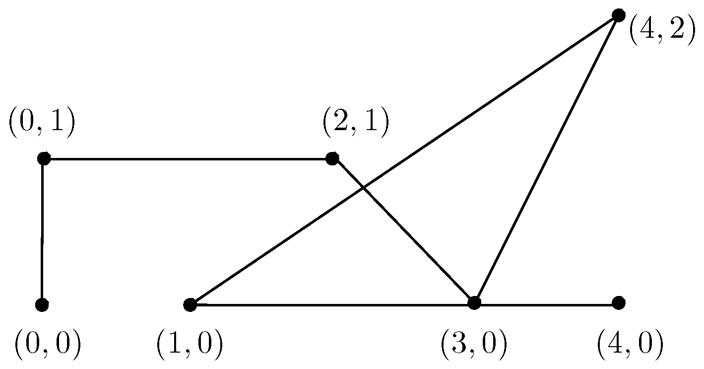
As an illustration we use the polyline P depicted in Figure 14. Here, the local carrier orders in the vertices are given by:

• $\mathsf{LCO}(P,{\mathsf{p}}_0)=\langle \left\{\right\},\left\{\overline{{\mathsf{p}}_0{\mathsf{p}}_1}\right\},\{\overline{{\mathsf{p}}_0{\mathsf{p}}_2},\overline{{\mathsf{p}}_0{\mathsf{p}}_4}\},\left\{\right\},\left\{\right\},\left\{\right\},\left\{\right\},\left\{\right\},\left\{\overline{{\mathsf{p}}_0{\mathsf{p}}_3}\right\}\rangle$
• $\mathsf{LCO}(P,{\mathsf{p}}_1)=\langle \left\{\right\},\left\{\overline{{\mathsf{p}}_1{\mathsf{p}}_2}\right\},\left\{\right\},\left\{\right\},\left\{\overline{{\mathsf{p}}_1{\mathsf{p}}_0}\right\},\left\{\right\},\left\{\right\},\left\{\right\},\{\overline{{\mathsf{p}}_1{\mathsf{p}}_3},\overline{{\mathsf{p}}_1{\mathsf{p}}_4}\}\rangle$
• $\mathsf{LCO}(P,{\mathsf{p}}_2)=\langle \left\{\right\},\left\{\overline{{\mathsf{p}}_2{\mathsf{p}}_3}\right\},\left\{\overline{{\mathsf{p}}_2{\mathsf{p}}_4}\right\},\left\{\right\},\left\{\right\},\left\{\right\},\left\{\overline{{\mathsf{p}}_2{\mathsf{p}}_0}\right\},\left\{\right\},\left\{\right\}\rangle$
• $\mathsf{LCO}(P,{\mathsf{p}}_3)=\langle \left\{\right\},\left\{\overline{{\mathsf{p}}_3{\mathsf{p}}_4}\right\},\left\{\overline{{\mathsf{p}}_3{\mathsf{p}}_2}\right\},\left\{\right\},\{\overline{{\mathsf{p}}_3{\mathsf{p}}_1},\overline{{\mathsf{p}}_3{\mathsf{p}}_0}\},\left\{\right\},\left\{\right\},\left\{\right\},\left\{\right\}\rangle$

We now define the notion of local-carrier-order similarity of two polylines.

Definition 17. 

Let $P=\langle {\mathsf{p}}_0,{\mathsf{p}}_1,\cdots ,{\mathsf{p}}_N\rangle$ and $Q=\langle {\mathsf{q}}_0,{\mathsf{q}}_1,\cdots ,{\mathsf{q}}_N\rangle$ be polylines of equal size. We say that P and Q are local-carrier-order similar if $\mathsf{LCO}(P,{\mathsf{p}}_i)=\mathsf{LCO}(Q,{\mathsf{q}}_i)$ for all $i=0,1,...,N-1$, that is, if $\mathsf{LCO}\left(P\right)=\mathsf{LCO}\left(Q\right)$ (always, modulo changing ${\mathsf{p}}_i$ in ${\mathsf{q}}_i$).

5.2. An Algebraic Characterization of the Local Carrier Order of a Polyline

In this section, we give algebraic conditions to express the local carrier order of a polyline. Hereto, it suffices to give for each vertex ${\mathsf{p}}_i$, with $0\le i<N$, in the polyline $P=\langle {\mathsf{p}}_0,{\mathsf{p}}_1,\cdots ,{\mathsf{p}}_N\rangle$ characterizations of the sets in the list

$$\langle \mathsf{Eq}\left({\mathsf{p}}_i\right),\mathsf{N}\left({\mathsf{p}}_i\right),\mathsf{NE}\left({\mathsf{p}}_i\right),\mathsf{E}\left({\mathsf{p}}_i\right),\mathsf{SE}\left({\mathsf{p}}_i\right),\mathsf{S}\left({\mathsf{p}}_i\right),\mathsf{SW}\left({\mathsf{p}}_i\right),\mathsf{W}\left({\mathsf{p}}_i\right),\mathsf{NW}\left({\mathsf{p}}_i\right)\rangle .$$

The following property gives this characterization. The proof of this property uses the same algebraic tools as the proof of Theorem 5 and we will skip the (straightforward) details.

We remark that, obviously, the algebraic characterisation of $\mathsf{Eq}\left({\mathsf{p}}_i\right)$ is given by equalities on the coordinates.

Proposition 18. 

Let $P=\langle ({\mathsf{x}}_0,{\mathsf{y}}_0),({\mathsf{x}}_1,{\mathsf{y}}_1),\cdots ,({\mathsf{x}}_N,{\mathsf{y}}_N)\rangle$ be a polyline and let ${\mathsf{p}}_i=({\mathsf{x}}_i,{\mathsf{y}}_i)$, for $0\le i\le N$. For $0\le j<i$ or $i<j<N$, the following table gives algebraic conditions for the halfline $\overline{{\mathsf{p}}_i{\mathsf{p}}_j}$ to belong to $\mathsf{X}\left({\mathsf{p}}_i\right)$ with $\mathsf{X}\in \{\mathsf{N},\mathsf{NE},\mathsf{E},\mathsf{SE},\mathsf{S},\mathsf{SW},\mathsf{W},\mathsf{NW}\}$:

$\mathsf{X}=$	$\overline{{\mathsf{p}}_i{\mathsf{p}}_j}\in \mathsf{X}\left({\mathsf{p}}_i\right)$ is equivalent to
$\mathsf{N}$	$-(({\mathsf{x}}_j-{\mathsf{x}}_i)·({\mathsf{x}}_{i+1}-{\mathsf{x}}_i)+({\mathsf{y}}_j-{\mathsf{y}}_i)·({\mathsf{y}}_{i+1}-{\mathsf{y}}_i))<0$
	and
	$-(({\mathsf{x}}_j-{\mathsf{x}}_i)·({\mathsf{y}}_{i+1}-{\mathsf{y}}_i)-({\mathsf{y}}_j-{\mathsf{y}}_i)·({\mathsf{x}}_{i+1}-{\mathsf{x}}_i))=0$
$\mathsf{NE}$	$-(({\mathsf{x}}_j-{\mathsf{x}}_i)·({\mathsf{x}}_{i+1}-{\mathsf{x}}_i)+({\mathsf{y}}_j-{\mathsf{y}}_i)·({\mathsf{y}}_{i+1}-{\mathsf{y}}_i))<0$
	and
	$-(({\mathsf{x}}_j-{\mathsf{x}}_i)·({\mathsf{y}}_{i+1}-{\mathsf{y}}_i)-({\mathsf{y}}_j-{\mathsf{y}}_i)·({\mathsf{x}}_{i+1}-{\mathsf{x}}_i))<0$
$\mathsf{E}$	$-(({\mathsf{x}}_j-{\mathsf{x}}_i)·({\mathsf{x}}_{i+1}-{\mathsf{x}}_i)+({\mathsf{y}}_j-{\mathsf{y}}_i)·({\mathsf{y}}_{i+1}-{\mathsf{y}}_i))=0$
	and
	$-(({\mathsf{x}}_j-{\mathsf{x}}_i)·({\mathsf{y}}_{i+1}-{\mathsf{y}}_i)-({\mathsf{y}}_j-{\mathsf{y}}_i)·({\mathsf{x}}_{i+1}-{\mathsf{x}}_i))<0$
$\mathsf{SE}$	$-(({\mathsf{x}}_j-{\mathsf{x}}_i)·({\mathsf{x}}_{i+1}-{\mathsf{x}}_i)+({\mathsf{y}}_j-{\mathsf{y}}_i)·({\mathsf{y}}_{i+1}-{\mathsf{y}}_i))>0$
	and
	$-(({\mathsf{x}}_j-{\mathsf{x}}_i)·({\mathsf{y}}_{i+1}-{\mathsf{y}}_i)-({\mathsf{y}}_j-{\mathsf{y}}_i)·({\mathsf{x}}_{i+1}-{\mathsf{x}}_i))<0$
$\mathsf{S}$	$-(({\mathsf{x}}_j-{\mathsf{x}}_i)·({\mathsf{x}}_{i+1}-{\mathsf{x}}_i)+({\mathsf{y}}_j-{\mathsf{y}}_i)·({\mathsf{y}}_{i+1}-{\mathsf{y}}_i))>0$
	and
	$-(({\mathsf{x}}_j-{\mathsf{x}}_i)·({\mathsf{y}}_{i+1}-{\mathsf{y}}_i)-({\mathsf{y}}_j-{\mathsf{y}}_i)·({\mathsf{x}}_{i+1}-{\mathsf{x}}_i))=0$
$\mathsf{SW}$	$-(({\mathsf{x}}_j-{\mathsf{x}}_i)·({\mathsf{x}}_{i+1}-{\mathsf{x}}_i)+({\mathsf{y}}_j-{\mathsf{y}}_i)·({\mathsf{y}}_{i+1}-{\mathsf{y}}_i))>0$
	and
	$-(({\mathsf{x}}_j-{\mathsf{x}}_i)·({\mathsf{y}}_{i+1}-{\mathsf{y}}_i)-({\mathsf{y}}_j-{\mathsf{y}}_i)·({\mathsf{x}}_{i+1}-{\mathsf{x}}_i))>0$
$\mathsf{W}$	$-(({\mathsf{x}}_j-{\mathsf{x}}_i)·({\mathsf{x}}_{i+1}-{\mathsf{x}}_i)+({\mathsf{y}}_j-{\mathsf{y}}_i)·({\mathsf{y}}_{i+1}-{\mathsf{y}}_i))=0$
	and
	$-(({\mathsf{x}}_j-{\mathsf{x}}_i)·({\mathsf{y}}_{i+1}-{\mathsf{y}}_i)-({\mathsf{y}}_j-{\mathsf{y}}_i)·({\mathsf{x}}_{i+1}-{\mathsf{x}}_i))>0$
$\mathsf{NW}$	$-(({\mathsf{x}}_j-{\mathsf{x}}_i)·({\mathsf{x}}_{i+1}-{\mathsf{x}}_i)+({\mathsf{y}}_j-{\mathsf{y}}_i)·({\mathsf{y}}_{i+1}-{\mathsf{y}}_i))<0$
	and
	$-(({\mathsf{x}}_j-{\mathsf{x}}_i)·({\mathsf{y}}_{i+1}-{\mathsf{y}}_i)-({\mathsf{y}}_j-{\mathsf{y}}_i)·({\mathsf{x}}_{i+1}-{\mathsf{x}}_i))>0$

5.3. A Characterization of Double-Cross Similarity of Polylines in Terms of Their Local Carrier Order

In this section, we give a geometric characterization of double-cross similarity of polylines in terms of their local carrier orders. The main theorem that we prove in this section is the following.

Theorem 19. 

Let P and Q be polylines of equal size. Then, P and Q are double-cross similar if and only if they are local-carrier-order similar. That is

$$\mathsf{DCM}\left(P\right)=\mathsf{DCM}\left(Q\right)ifandonlyif\mathsf{LCO}\left(P\right)=\mathsf{LCO}\left(Q\right).$$

The two directions of this theorem are proven in Lemma 20 and Lemma 22 (or their immediate Corollaries 21 and 23).

Lemma 20. 

Let $P=\langle {\mathsf{p}}_0,{\mathsf{p}}_1,\cdots ,{\mathsf{p}}_N\rangle$ be a polyline. For $i,j$ with $0\le i\le j<N$, we can derive the value of the 4-tuple $\mathsf{DCM}\left(P\right)[i,j]=\left(C_1{C}_2{C}_3{C}_4\right)$ from $\mathsf{LCO}(P,{\mathsf{p}}_i)$ and $\mathsf{LCO}(P,{\mathsf{p}}_j)$.

Proof. 

Let $P=\langle {\mathsf{p}}_0,{\mathsf{p}}_1,\cdots ,{\mathsf{p}}_N\rangle$ be a polyline of size N. If ${\mathsf{p}}_j\in \mathsf{Eq}\left({\mathsf{p}}_i\right)$, then $\mathsf{DCM}\left(P\right)[i,j]=\left(0000\right).$ This is in particular true if $i=j$.

If ${\mathsf{p}}_j\notin \mathsf{Eq}\left({\mathsf{p}}_i\right)$, then the following twelve easily observable facts show how to determine $C_1$, $C_2$, $C_3$ and $C_4$ (for instance, by a detailed inspection of Figure 5).

$C_1$	is equivalent to
0	$\overline{{\mathsf{p}}_i{\mathsf{p}}_j}\in \mathsf{W}\left({\mathsf{p}}_i\right)\cup \mathsf{E}\left({\mathsf{p}}_i\right)$
+	$\overline{{\mathsf{p}}_i{\mathsf{p}}_j}\in \mathsf{SE}\left({\mathsf{p}}_i\right)\cup \mathsf{S}\left({\mathsf{p}}_i\right)\cup \mathsf{SW}\left({\mathsf{p}}_i\right)$
−	$\overline{{\mathsf{p}}_i{\mathsf{p}}_j}\in \mathsf{NW}\left({\mathsf{p}}_i\right)\cup \mathsf{N}\left({\mathsf{p}}_i\right)\cup \mathsf{NE}\left({\mathsf{p}}_i\right)$
$C_2$	is equivalent to
0	$\overline{{\mathsf{p}}_j{\mathsf{p}}_i}\in \mathsf{W}\left({\mathsf{p}}_j\right)\cup \mathsf{E}\left({\mathsf{p}}_j\right)$
+	$\overline{{\mathsf{p}}_j{\mathsf{p}}_i}\in \mathsf{SE}\left({\mathsf{p}}_j\right)\cup \mathsf{S}\left({\mathsf{p}}_j\right)\cup \mathsf{SW}\left({\mathsf{p}}_j\right)$
−	$\overline{{\mathsf{p}}_i{\mathsf{p}}_j}\in \mathsf{NW}\left({\mathsf{p}}_i\right)\cup \mathsf{N}\left({\mathsf{p}}_i\right)\cup \mathsf{NE}\left({\mathsf{p}}_i\right)$
$C_3$	is equivalent to
0	$\overline{{\mathsf{p}}_i{\mathsf{p}}_j}\in \mathsf{N}\left({\mathsf{p}}_i\right)\cup \mathsf{S}\left({\mathsf{p}}_i\right)$
+	$\overline{{\mathsf{p}}_i{\mathsf{p}}_j}\in \mathsf{SW}\left({\mathsf{p}}_i\right)\cup \mathsf{W}\left({\mathsf{p}}_i\right)\cup \mathsf{NW}\left({\mathsf{p}}_i\right)$
−	$\overline{{\mathsf{p}}_i{\mathsf{p}}_j}\in \mathsf{NE}\left({\mathsf{p}}_i\right)\cup \mathsf{E}\left({\mathsf{p}}_i\right)\cup \mathsf{SE}\left({\mathsf{p}}_i\right)$
$C_4$	is equivalent to
0	$\overline{{\mathsf{p}}_i{\mathsf{p}}_j}\in \mathsf{N}\left({\mathsf{p}}_j\right)\cup \mathsf{S}\left({\mathsf{p}}_j\right)$
+	$\overline{{\mathsf{p}}_i{\mathsf{p}}_j}\in \mathsf{SW}\left({\mathsf{p}}_j\right)\cup \mathsf{W}\left({\mathsf{p}}_j\right)\cup \mathsf{NW}\left({\mathsf{p}}_j\right)$
−	$\overline{{\mathsf{p}}_i{\mathsf{p}}_j}\in \mathsf{NE}\left({\mathsf{p}}_i\right)\cup \mathsf{E}\left({\mathsf{p}}_i\right)\cup \mathsf{SE}\left({\mathsf{p}}_i\right)$

This concludes the proof.

This lemma has the following immediate corollary.

Corollary 21. 

Let P be a polyline in ${\mathbf{R}}^2$. Then, the matrix $\mathsf{DCM}\left(P\right)$ can be reconstructed from the local carrier order $\mathsf{LCO}\left(P\right)$.

Proof. 

Properties 7 and 8 show that it is sufficient to know a double-cross matrix of a polyline on and above its diagonal in order to complete it below its diagonal. And Lemma 20 shows how the local carrier order gives the double-cross matrix on and above its diagonal. This concludes the proof.

Now, we turn to the other implication of Theorem 19.

Lemma 22. 

Let $P=\langle {\mathsf{p}}_0,{\mathsf{p}}_1,\cdots ,{\mathsf{p}}_N\rangle$ be a polyline in ${\mathbf{R}}^2$ of size N. If $0\le i<j<N$, then $\mathsf{DCM}\left(P\right)[i,j]$ contains enough information to derived to which set of $\mathsf{LCO}(P,{\mathsf{p}}_i)$ the half-lines $\overline{{\mathsf{p}}_i{\mathsf{p}}_j}$ belong and to which set of $\mathsf{LCO}(P,{\mathsf{p}}_j)$ the half-lines $\overline{{\mathsf{p}}_j{\mathsf{p}}_i}$ belong.

Proof. 

Let $\mathsf{DCM}\left(P\right)[i,j]=\left(C_1{C}_2{C}_3{C}_4\right)$, for $0\le i<j<N$. Again, the following facts are easily observable (for instance, by a detailed inspection of Figure 5).

$C_1$	$C_3$	is equivalent to		$C_2$	$C_4$	is equivalent to
−	−	$\overline{{\mathsf{p}}_i{\mathsf{p}}_j}\in \mathsf{NE}\left({\mathsf{p}}_i\right)$		−	−	$\overline{{\mathsf{p}}_j{\mathsf{p}}_i}\in \mathsf{NE}\left({\mathsf{p}}_j\right)$
−	0	$\overline{{\mathsf{p}}_i{\mathsf{p}}_j}\in \mathsf{N}\left({\mathsf{p}}_i\right)$		−	0	$\overline{{\mathsf{p}}_j{\mathsf{p}}_i}\in \mathsf{N}\left({\mathsf{p}}_j\right)$
−	+	$\overline{{\mathsf{p}}_i{\mathsf{p}}_j}\in \mathsf{NW}\left({\mathsf{p}}_i\right)$		−	+	$\overline{{\mathsf{p}}_j{\mathsf{p}}_i}\in \mathsf{NW}\left({\mathsf{p}}_j\right)$
0	−	$\overline{{\mathsf{p}}_i{\mathsf{p}}_j}\in \mathsf{E}\left({\mathsf{p}}_i\right)$		0	−	$\overline{{\mathsf{p}}_j{\mathsf{p}}_i}\in \mathsf{E}\left({\mathsf{p}}_j\right)$
0	0	${\mathsf{p}}_i={\mathsf{p}}_{i+1}$ is excluded		0	0	${\mathsf{p}}_j={\mathsf{p}}_{j+1}$ is excluded
0	+	$\overline{{\mathsf{p}}_i{\mathsf{p}}_j}\in \mathsf{W}\left({\mathsf{p}}_i\right)$		0	+	$\overline{{\mathsf{p}}_j{\mathsf{p}}_i}\in \mathsf{W}\left({\mathsf{p}}_j\right)$
+	−	$\overline{{\mathsf{p}}_i{\mathsf{p}}_j}\in \mathsf{SE}\left({\mathsf{p}}_i\right)$		+	−	$\overline{{\mathsf{p}}_j{\mathsf{p}}_i}\in \mathsf{SE}\left({\mathsf{p}}_j\right)$
+	0	$\overline{{\mathsf{p}}_i{\mathsf{p}}_j}\in \mathsf{S}\left({\mathsf{p}}_i\right)$		+	0	$\overline{{\mathsf{p}}_j{\mathsf{p}}_i}\in \mathsf{S}\left({\mathsf{p}}_j\right)$
+	+	$\overline{{\mathsf{p}}_i{\mathsf{p}}_j}\in \mathsf{SW}\left({\mathsf{p}}_i\right)$		+	+	$\overline{{\mathsf{p}}_j{\mathsf{p}}_i}\in \mathsf{SW}\left({\mathsf{p}}_j\right)$

This concludes the proof.

This lemma has the following immediate corollary.

Corollary 23. 

Given $\mathsf{DCM}\left(P\right)$, $\mathsf{LCO}(P,{\mathsf{p}}_i)$ can be constructed for all $0\le i<N$.

Combined, Corollaries 21 and 23 prove Theorem 19.

6. A Characterization of the Double-Cross Invariant Transformations of the Plane

In this section, we identify the transformations of the plane ${\mathbf{R}}^2$ that leave the double-cross matrix of all polylines invariant. By a transformation we mean a continuous, bijective mapping of the plane ${\mathbf{R}}^2$ onto itself.

If $\alpha :{\mathbf{R}}^2\to {\mathbf{R}}^2$ is a transformation and if $\mathsf{p}$ and $\mathsf{q}$ are points in ${\mathbf{R}}^2$, then we write $\alpha (\overrightarrow{\mathsf{p}\mathsf{q}})$ for $\overrightarrow{\alpha \left(\mathsf{p}\left)\alpha \right(\mathsf{q}\right)}$.

What do we mean by applying a transformation of the plane to a polyline? The following definition says that we mean it to be the polyline formed by the transformed vertices.

Definition 24. 

Let $\alpha :{\mathbf{R}}^2\to {\mathbf{R}}^2$ be a transformation. Let $P=\langle ({\mathsf{x}}_0,{\mathsf{y}}_0),({\mathsf{x}}_1,{\mathsf{y}}_1),\cdots ,({\mathsf{x}}_N,{\mathsf{y}}_N)\rangle$ be a polyline. We define $\alpha \left(P\right)$ to be the polyline $\langle \alpha ({\mathsf{x}}_0,{\mathsf{y}}_0),\alpha ({\mathsf{x}}_1,{\mathsf{y}}_1),\cdots ,\alpha ({\mathsf{x}}_N,{\mathsf{y}}_N)\rangle .$

We remark that since a transformation α is a bijective function, the assumption in Definition 1, which says that no two consecutive vertices of a polyline are identical, will hold for $\alpha \left(P\right)$ if it holds for the polyline P.

We now define the notion of double-cross invariant transformation of the plane.

Definition 25. 

Let $\alpha :{\mathbf{R}}^2\to {\mathbf{R}}^2$ be a transformation. Let P be a polyline. We say that α leaves P invariant if P and $\alpha \left(P\right)$ are double-cross similar, that is, if $\mathsf{DCM}\left(P\right)=\mathsf{DCM}\left(\alpha \right(P\left)\right)$.

We say that α is a double-cross invariant transformation if it leaves all polylines invariant. A group of transformations of ${\mathbf{R}}^2$ is double-cross invariant if all its members are double-cross invariant transformations.

The main aim of this section is to prove the following theorem, which says that the largest group of transformations that is double-cross invariant consists of the translations, rotations and homotecies (or scalings) of the plane. The elements of this group are called the similarities of ${\mathbf{R}}^2$. We remark that a homotecy of the plane is a transformation of the form ${\alpha }_{\mathsf{c}}:{\mathbf{R}}^2\to {\mathbf{R}}^2:(x,y)\mapsto \mathsf{c}·(x,y)$, where $c\in \mathbf{R}$ and $\mathsf{c}\ne 0$.

Theorem 26. 

The largest group of transformations of ${\mathbf{R}}^2$, that is double-cross invariant consist of the similarity transformations of the plane onto itself, that is, transformations of the form

$$\alpha :{\mathbf{R}}^2\to {\mathbf{R}}^2:\left(\begin{array}{c}x\\ y\end{array}\right)\mapsto \mathsf{c}·\left(\begin{array}{cc}\mathsf{a}& \hfill -\mathsf{b}\\ \mathsf{b}& \hfill \mathsf{a}\end{array}\right)·\left(\begin{array}{c}x\\ y\end{array}\right)+\left(\begin{array}{c}\mathsf{d}\\ \mathsf{e}\end{array}\right),$$

where $\mathsf{a},\mathsf{b},\mathsf{c},\mathsf{d},\mathsf{e}\in \mathbf{R}$, $\mathsf{c}\ne 0$ and ${\mathsf{a}}^2+{\mathsf{b}}^2=1$.

We remark that the condition ${\mathsf{a}}^2+{\mathsf{b}}^2=1$ imply that the matrix is orthogonal and that $\mathsf{a}$ and $\mathsf{b}$ cannot be both zero. In fact, we can see $\mathsf{a}$ as $cos\phi$ and $\mathsf{b}$ as $sin\phi$, where φ is the angle of the rotation expressed by the matrix.

We prove this theorem by proving three lemma’s. Lemma 27 proves soundness and Lemma 29 proves completeness. Lemma 28 is a purely technical lemma.

Lemma 27. 

The translations, rotations and homotecies of the plane (that is, the transformations given in Theorem 5) are double-cross invariant transformations.

Proof. 

We consider the three types of transformations separately, since we can apply them one after the other. In all cases, we use the algebraic characterization, given by Theorem 5.

1. Translations. We have already remarked that all the factors appearing in the algebraic expressions, given by given by Theorem 5, that is $({\mathsf{x}}_j-{\mathsf{x}}_i)$, $({\mathsf{x}}_{i+1}-{\mathsf{x}}_i)$, $({\mathsf{y}}_j-{\mathsf{y}}_i)$, $({\mathsf{y}}_{i+1}-{\mathsf{y}}_i)$, $({\mathsf{x}}_{j+1}-{\mathsf{x}}_j)$ and $({\mathsf{y}}_{j+1}-{\mathsf{y}}_j)$ are differences in x-coordinates or differences in y-coordinates. A translation ${\tau }_{(\mathsf{d},\mathsf{e})}:{\mathbf{R}}^2\to {\mathbf{R}}^2:(x,y)\mapsto (x+\mathsf{d},y+\mathsf{e})$, therefore leaves these differences unaltered. For instance, $({\mathsf{x}}_j-{\mathsf{x}}_i)$ is transformed to $({\mathsf{x}}_j+\mathsf{d}-({\mathsf{x}}_i+\mathsf{d}))$, which is, of course, the original value $({\mathsf{x}}_j-{\mathsf{x}}_i)$. None of the expressions given by Theorem 5 are therefore changed and the double-cross condition remain the same.

2. Rotations. Let

$${\rho }_{(\mathsf{a},\mathsf{b})}:{\mathbf{R}}^2\to {\mathbf{R}}^2:\left(\begin{array}{c}x\\ y\end{array}\right)\mapsto \left(\begin{array}{cc}\mathsf{a}& \hfill -\mathsf{b}\\ \mathsf{b}& \hfill \mathsf{a}\end{array}\right)·\left(\begin{array}{c}x\\ y\end{array}\right),$$

with ${\mathsf{a}}^2+{\mathsf{b}}^2=1$, be a rotation (that fixes the origin).

The expression for $C_1$ is transformed to

$$(\mathsf{a}·({\mathsf{x}}_j-{\mathsf{x}}_i)-\mathsf{b}·({\mathsf{y}}_j-{\mathsf{y}}_i))·(\mathsf{a}·({\mathsf{x}}_{i+1}-{\mathsf{x}}_i)-\mathsf{b}·({\mathsf{y}}_{i+1}-{\mathsf{y}}_i))+(\mathsf{b}·({\mathsf{x}}_j-{\mathsf{x}}_i)+\mathsf{a}·({\mathsf{y}}_j-{\mathsf{y}}_i)))·(\mathsf{b}·({\mathsf{x}}_{i+1}-{\mathsf{x}}_i)+\mathsf{a}·({\mathsf{y}}_{i+1}-{\mathsf{y}}_i)),$$

which simplifies to $({\mathsf{a}}^2+{\mathsf{b}}^2)·(({\mathsf{x}}_j-{\mathsf{x}}_i)·({\mathsf{x}}_{i+1}-{\mathsf{x}}_i)+({\mathsf{y}}_j-{\mathsf{y}}_i)·({\mathsf{y}}_{i+1}-{\mathsf{y}}_i))$, which is the original polynomial since ${\mathsf{a}}^2+{\mathsf{b}}^2=1$. For $C_2$, $C_3$ and $C_4$, a similar straightforward computation shows that the polynomials remain the same.

3. Homotecies. A homotecy ${\alpha }_{\mathsf{c}}:{\mathbf{R}}^2\to {\mathbf{R}}^2:(x,y)\mapsto \mathsf{c}·(x,y)$, transforms the differences $({\mathsf{x}}_j-{\mathsf{x}}_i)$, $({\mathsf{x}}_{i+1}-{\mathsf{x}}_i)$, $({\mathsf{y}}_j-{\mathsf{y}}_i)$, $({\mathsf{y}}_{i+1}-{\mathsf{y}}_i)$, $({\mathsf{x}}_{j+1}-{\mathsf{x}}_j)$ and $({\mathsf{y}}_{j+1}-{\mathsf{y}}_j)$ to $(\mathsf{c}·{\mathsf{x}}_j-\mathsf{c}·{\mathsf{x}}_i)$, $(\mathsf{c}·{\mathsf{x}}_{i+1}-\mathsf{c}·{\mathsf{x}}_i)$, $(\mathsf{c}·{\mathsf{y}}_j-\mathsf{c}·{\mathsf{y}}_i)$, $(\mathsf{c}·{\mathsf{y}}_{i+1}-\mathsf{c}·{\mathsf{y}}_i)$, $(\mathsf{c}·{\mathsf{x}}_{j+1}-\mathsf{c}·{\mathsf{x}}_j)$ and $(\mathsf{c}·{\mathsf{y}}_{j+1}-\mathsf{c}·{\mathsf{y}}_j)$. This means that the polynomials given by Theorem 5 are multiplied by ${\mathsf{c}}^2$, which is strictly larger than zero, for $\mathsf{c}\ne 0$. The signs of these polynomials are therefore unaltered. And the double-cross value of the scaled polyline is the same as the original one.

Before we can turn to completeness, we need the following technical lemma.

Lemma 28. 

Let $f:\mathbf{R}\to \mathbf{R}:t\mapsto f\left(t\right)$ be a strictly monotone increasing function. If

$$f(\frac{s+t}{2})=\frac{f\left(s\right)+f\left(t\right)}{2}$$

for any $s,t\in \mathbf{R}$, then $f\left(t\right)=\left(f\right(1)-f(0\left)\right)·t+f\left(0\right)$.

Proof. 

Suppose that f is a function as described and suppose that there is a $t_0\in \mathbf{R}$ such that $f\left(t_0\right)\ne (f\left(1\right)-f\left(0\right))·t_0+f\left(0\right)$. We remark that therefore $t_0$ cannot be 0 or 1.

If $f(-t_0)=(f\left(1\right)-f\left(0\right))·(-t_0)+f\left(0\right)$, then it follows from $2·f\left(0\right)=2·f(\frac{t_0-t_0}{2})=f\left(t_0\right)+f(-t_0)$ that also $f\left(t_0\right)=(f\left(1\right)-f\left(0\right))·t_0+f\left(0\right)$. We may therefore assume $0<t_0$.

If $f(\frac{t_0}{2})=(f\left(1\right)-f\left(0\right))·(\frac{t_0}{2})+f\left(0\right)$, then it follows from $2·f(\frac{0+t_0}{2})=f\left(0\right)+f\left(t_0\right)$ that also $f\left(t_0\right)=(f\left(1\right)-f\left(0\right))·t_0+f\left(0\right)$. We may therefore assume $0<t_0<1$.

Claim. 

For any $n\in \mathbf{N}$ and any k, with $0\le k\le 2^n$, we have that

$$f(\frac{k}{2^n})=(f\left(1\right)-f\left(0\right))·\frac{k}{2^n}+f\left(0\right).$$

We first prove this claim (by induction on n). For $n=0$, and $k=0,1$, we respectively have $f\left(0\right)=\left(f\right(1)-f(0\left)\right)·0+f\left(0\right)$ and $f\left(1\right)=\left(f\right(1)-f(0\left)\right)·1+f\left(0\right).$

Assume now that the claim is true for n. We prove it holds for $n+1$. We consider $\frac{k}{2^{n+1}}$ and distinguish between the cases, $0\le k\le 2^n$ and $k=k^{\prime }+2^n$ with $0<k^{\prime }\le 2^n$. If $0\le k\le 2^n$, then $f(\frac{k}{2^{n+1}})=f\left(\frac{1}{2}(0+\frac{k}{2^n})\right)=\frac{1}{2}(f\left(0\right)+f\left(\frac{k}{2^n}\right))$, which by the induction hypothesis equals $\frac{1}{2}(f\left(0\right)+(f\left(1\right)-f\left(0\right))·\frac{k}{2^n}+f\left(0\right))$ or $(f\left(1\right)-f\left(0\right))·\frac{k}{2^{n+1}}+f\left(0\right)$.

If $k=k^{\prime }+2^n$ with $0<k^{\prime }\le 2^n$, then $f(\frac{2^n+k^{\prime }}{2^{n+1}})=f(\frac{1}{2}(1+\frac{k^{\prime }}{2^n}))=\frac{1}{2}(f\left(1\right)+f(\frac{k^{\prime }}{2^n}))$, which by the induction hypothesis equals $\frac{1}{2}(f\left(1\right)+(f\left(1\right)-f\left(0\right))·\frac{k^{\prime }}{2^n}+f\left(0\right))$ which equals $\frac{1}{2}(f\left(1\right)-f\left(0\right))+(f\left(1\right)-f\left(0\right))·\frac{k^{\prime }}{2^{n+1}}+f\left(0\right)$ or $(f\left(1\right)-f\left(0\right))·\frac{k^{\prime }+2^n}{2^{n+1}}+f\left(0\right)$ which is $(f\left(1\right)-f\left(0\right))·\frac{k}{2^{n+1}}+f\left(0\right)$. This concludes the proof of the claim.

To conclude the proof, let $0<t_0<1$ and assume first that $f\left(t_0\right)>(f\left(1\right)-f\left(0\right))·t_0+f\left(0\right)$. This means that $t_0<\frac{f\left(t_0\right)-f\left(0\right)}{f\left(1\right)-f\left(0\right)}$. We remark that since f is assumed to be strictly monotone, $f\left(1\right)-f\left(0\right)\ne 0$ and therefore the division is allowed. Choose k and n such that

$$\frac{k}{2^n}\le t_0<\frac{k+1}{2^n}<\frac{f\left(t_0\right)-f\left(0\right)}{f\left(1\right)-f\left(0\right)},$$

with $0\le k\le 2^n$. Then $f(\frac{k+1}{2^n})=(f\left(1\right)-f\left(0\right))·\frac{k+1}{2^n}+f\left(0\right)<f\left(t_0\right)$, although $t_0<\frac{k+1}{2^n}$, which contradicts the fact that f is strictly monotone increasing.

If we assume $f\left(t_0\right)<(f\left(1\right)-f\left(0\right))·t_0+f\left(0\right)$ on the other hand, we have $\frac{f\left(t_0\right)-f\left(0\right)}{f\left(1\right)-f\left(0\right)}<t_0$. Choose k and n such that

$$\frac{f\left(t_0\right)-f\left(0\right)}{f\left(1\right)-f\left(0\right)}<\frac{k}{2^n}<t_0\le \frac{k+1}{2^n},$$

with $0\le k\le 2^n$. Then $f\left(\frac{k}{2^n}\right)=(f\left(1\right)-f\left(0\right))·\frac{k}{2^n}+f\left(0\right)>f\left(t_0\right)$, although $\frac{k}{2^n}<t_0$, which contradicts the fact that f is strictly monotone increasing. In both cases, we obtain a contradiction and this concludes the proof.

The following lemma proves completeness. The proof is kept elementary and we remark that it shows how the double-cross formalism can be used to construct midpoints.

Lemma 29. 

The similarity transformations of the plane (given in Theorem 5) are the only double-cross invariant transformations.

Proof. 

Let $\alpha :{\mathbf{R}}^2\to {\mathbf{R}}^2$ be a double-cross invariant transformation.

(1) We consider polylines $P=\langle {\mathsf{p}}_0,{\mathsf{p}}_1,{\mathsf{p}}_2\rangle ,$ where ${\mathsf{p}}_0$, ${\mathsf{p}}_1$ and ${\mathsf{p}}_2$ are collinear points with ${\mathsf{p}}_1$ between ${\mathsf{p}}_0$ and ${\mathsf{p}}_2$. By the assumption in Definition 1, ${\mathsf{p}}_1$ should be strictly between ${\mathsf{p}}_0$ and ${\mathsf{p}}_2$ The only relevant entry in the double-cross matrix of this polyline is $\mathsf{DC}(\overrightarrow{{\mathsf{p}}_0{\mathsf{p}}_1},\overrightarrow{{\mathsf{p}}_1{\mathsf{p}}_2})$ which is $(-+00)$. In $\alpha \left(P\right)$, $\mathsf{DC}(\alpha (\overrightarrow{{\mathsf{p}}_0{\mathsf{p}}_1}),\alpha (\overrightarrow{{\mathsf{p}}_1{\mathsf{p}}_2}))$ should also be $(-+00)$. This implies that $\alpha \left({\mathsf{p}}_0\right)$, $\alpha \left({\mathsf{p}}_1\right)$ and $\alpha \left({\mathsf{p}}_2\right)$ should also be collinear, with $\alpha \left({\mathsf{p}}_1\right)$ (strictly) between $\alpha \left({\mathsf{p}}_0\right)$ and $\alpha \left({\mathsf{p}}_2\right)$. This means that α preserves collinearity and betweenness, depicted in Figure 15.

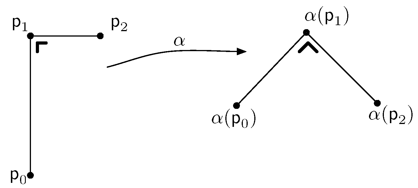
(2) We consider polylines $P=\langle {\mathsf{p}}_0,{\mathsf{p}}_1,{\mathsf{p}}_2\rangle ,$ where $\angle (\overrightarrow{{\mathsf{p}}_1{\mathsf{p}}_0},\overrightarrow{{\mathsf{p}}_1{\mathsf{p}}_2})={90}^{\circ }$, that is, the polyline takes a right turn at ${\mathsf{p}}_1$. The only relevant entry in the double-cross matrix of this polyline is again $\mathsf{DC}(\overrightarrow{{\mathsf{p}}_0{\mathsf{p}}_1},\overrightarrow{{\mathsf{p}}_1{\mathsf{p}}_2})$ which is now $(-00-)$. In $\alpha \left(P\right)$, $\mathsf{DC}(\alpha (\overrightarrow{{\mathsf{p}}_0{\mathsf{p}}_1}),\alpha (\overrightarrow{{\mathsf{p}}_1{\mathsf{p}}_2}))$ should also be $(-00-)$. This means that α is a right-turn-preserving transformation. This is illustrated in Figure 16. Similarly, α is a left-turn-preserving transformation.

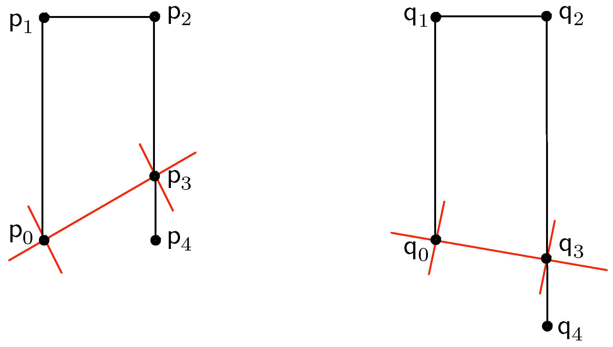
(3) We consider the polyline $P=\langle {\mathsf{p}}_0,{\mathsf{p}}_1,{\mathsf{p}}_2,{\mathsf{p}}_3,{\mathsf{p}}_4,{\mathsf{p}}_5,{\mathsf{p}}_6,{\mathsf{p}}_7,{\mathsf{p}}_8,{\mathsf{p}}_9,{\mathsf{p}}_{10},{\mathsf{p}}_{11},{\mathsf{p}}_{12}\rangle ,$ with ${\mathsf{p}}_0={\mathsf{p}}_4={\mathsf{p}}_7={\mathsf{p}}_{12}(0,0)$, ${\mathsf{p}}_1={\mathsf{p}}_5=(0,1)$, ${\mathsf{p}}_2={\mathsf{p}}_{10}=(1,1)$, ${\mathsf{p}}_3={\mathsf{p}}_8=(1,0)$ and ${\mathsf{p}}_6={\mathsf{p}}_9=(\frac{1}{2},\frac{1}{2})$, depicted in Figure 17. This polyline forms a square with its two diagonals after making six ${90}^{\circ }$ right-turns and two ${90}^{\circ }$ left-turns . It is also closed in the sense that its start and end vertex are equal. The transformation α, which according to (2) preserves right and left turns, therefore has to map P again to a square with its diagonals. This means α is a square-preserving transformation. In particular, α preserves parallel line segments. Also, ${\mathsf{p}}_6$, which is the midpoint between ${\mathsf{p}}_0$ and ${\mathsf{p}}_2$ is mapped to $\alpha \left({\mathsf{p}}_6\right)$, which should be the midpoint between $\alpha \left({\mathsf{p}}_0\right)$ and $\alpha \left({\mathsf{p}}_2\right)$. This means α is a midpoint-preserving transformation.

Suppose $\alpha (0,0)=(a,b)$. If ${\tau }_{(-a,-b)}$ is the translation $(x,y)\mapsto (x-a,y-b)$, then ${\tau }_{(-a,-b)}\circ \alpha (0,0)=(0,0)$. Suppose ${\tau }_{(-a,-b)}\circ \alpha (1,0)=(c,d)$. Let ${\rho }_{(c,d)}$ be the rotation with $(0,0)$ as center that brings $(c,d)$ to the positive x-axis, that is, to $(\sqrt{c^2+d^2},0)$. We remark that $(c,d)$ cannot be the origin since α is assumed to be a bijective function. So, also ${\tau }_{(-a,-b)}\circ \alpha$ is bijective. Furthermore, let ${\sigma }_{\sqrt{c^2+d^2}}$ be the scaling $(x,y)\mapsto \frac{1}{\sqrt{c^2+d^2}}(x,y)$ and let

$$\beta ={\sigma }_{\sqrt{c^2+d^2}}\circ {\rho }_{(c,d)}\circ {\tau }_{(-a,-b)}\circ \alpha .$$

Then we have that $\beta (0,0)=(0,0)$ and $\beta (1,0)=(1,0)$.

Since α is a double-cross invariant transformation, by assumption, and since ${\sigma }_{\sqrt{c^2+d^2}}$, ${\rho }_{(c,d)}$ and ${\tau }_{(-a,-b)}$ are double-cross invariant transformations by Lemma 27, also β is a double-cross invariant transformation. And β also inherits from α the properties of preserving betweenness, collinearity, right- and left turns, squares, parallel line segments and midpoints. Because β preserves squares, we also have $\beta (0,1)=(0,1)$.

We now claim the following.

Claim. 

The transformation β is the identity.

The proof of this claim finishes the proof. Indeed, then we have

$$\alpha ={\sigma }_{\sqrt{c^2+d^2}}^{-1}\circ {\rho }_{(c,d)}^{-1}\circ {\tau }_{(-a,-b)}^{-1},$$

which is of the required form.

Proof of the claim: First, we show that β is the identity on the x-axis and next we do the same for all lines perpendicular to the x-axis. Hereto, we consider the function

$${\beta }_x:\mathbf{R}\to \mathbf{R}:x\mapsto {\beta }_x\left(x\right):={\pi }_x\left(\beta (x,0)\right),$$

where ${\pi }_x$ is the projection on the first component, that is, ${\pi }_x(x,y):=x$. Since $\beta (0,0)=(0,0)$ and $\beta (1,0)=(1,0)$ and β preserves collinearity, β maps the x-axis onto the x-axis and we have ${\beta }_x\left(0\right)=0$ and ${\beta }_x\left(1\right)=1$. Furthermore, since β and hence ${\beta }_x$ preserves betweenness, ${\beta }_x$ is strictly monotone increasing. Indeed, let $s,t\in \mathbf{R}$ with $s<t$. With respect to 0 and 1, we can consider the twelve possible locations of s and t: $s<t<0$; $s<t=0<1$; $s<0<t<1$; $s<0<t=1$; $s<0<1<t$; $s=0<t<1$; $s=0<t=1$; $s=0<1<t$; $0<s<t=1$; $0<s<1<t$; $0<s=1<t$; and $0<1<s<t$. In all cases, except $s=0<t=1$, we have three points. So, here we can use the fact that β preserves betweenness to show that ${\beta }_x\left(s\right)<{\beta }_x\left(t\right)$. In the case $s=0<t=1$, we have ${\beta }_x\left(s\right)={\beta }_x\left(0\right)=0<1={\beta }_x\left(1\right)={\beta }_x\left(t\right).$ Finally, since β preserves midpoints, also for ${\beta }_x$, we have

$${\beta }_x(\frac{s+t}{2})=\frac{{\beta }_x\left(s\right)+{\beta }_x\left(t\right)}{2},$$

for all $s,t\in \mathbf{R}$. All the conditions to apply Lemma 28 are therefore fulfilled. And we get ${\beta }_x\left(x\right)=({\beta }_x\left(1\right)-{\beta }_x\left(0\right))·x+{\beta }_x\left(0\right)=(1-0)·x+0=x.$

Now, we fix some ${\mathsf{x}}_0\in \mathbf{R}$ and consider the function

$${\beta }_{{\mathsf{x}}_0,y}:\mathbf{R}\to \mathbf{R}:y\mapsto {\beta }_{{\mathsf{x}}_0,y}\left(y\right):={\pi }_y\left(\beta ({\mathsf{x}}_0,y)\right),$$

where ${\pi }_y(x,y):=y.$ Since β preserves parallel line segments, ${\beta }_{{\mathsf{x}}_0,y}$ maps the line with equation $x={\mathsf{x}}_0$ onto itself (since it maps the y-axis to itself). Since β also preserves the rectangle given by the polyline

$$P=\langle (0,0),(0,1),(1,1),({\mathsf{x}}_0,1),({\mathsf{x}}_0,0),(1,0),(0,0),(0,1)\rangle$$

(for ${\mathsf{x}}_0=1$, we can omit $({\mathsf{x}}_0,1)$ and $({\mathsf{x}}_0,0)$ from the list) onto itself, we have again have ${\beta }_{{\mathsf{x}}_0,y}\left(0\right)=0$ and ${\beta }_{{\mathsf{x}}_0,y}\left(1\right)=1$. The function ${\beta }_{{\mathsf{x}}_0,y}$ also inherits from β the property of preserving midpoints and is strictly monotonic increasing on the line $x={\mathsf{x}}_0$. So, again we can apply Lemma 28 to show that ${\beta }_{{\mathsf{x}}_0,y}$ is the identity.

Since $\beta (x,y)=({\beta }_x\left(x\right),{\beta }_{x,y}\left(y\right))$, we obtain that β is the identity transformation. This finishes the proof of the claim and also of the lemma.

7. Conclusions

We have studied the double-cross matrix descriptions of polylines in the two-dimensional plane from an algebraic and geometrical point of view. We have first given an algebraic characterization of the double-cross matrix of a polyline. This algebraic characterisation allowed us to prove some basic properties of double-cross matrices. We have given a geometric characterization of double-cross similarity of two polylines by means of the notion of the local carrier orders of polylines. Finally, we identify the transformations of the plane that leave the double-cross matrix of all polylines in the two-dimensional plane invariant.

Research on double-cross matrices gives rise to many questions of which we name a few here. Firstly, variants of double crosses can be imagined, for instance, to include the temporal dimension of moving object data. Another variant would be to rotate the double cross by ${45}^{\circ }$. This would make notions of straight ahead, back, right and left more relative. We can also envisage double crosses with a finer structure. They may have 8, 16 or more lines determining the “crosses”, as in the ${\mathrm{OPRA}}_n$-approach [29] (in some sense, the double-cross formalism can be seen as ${\mathrm{OPRA}}_2$).

Our algebraic characterization of the double-cross matrix of a polyline, also raises the question of the realisability of double-cross matrices. This question adds up to the following: given an $N\times N$ matrix of 4-tuples over the set $\{-,0,+\}$, decide if this is the double-cross matrix of a polyline. A matrix where $\left(0000\right)$ doesn’t appear on the diagonal, for instance, cannot be the double-cross matrix of a polyline. This decision problem leads to non-trivial problems in computational algebraic geometry.

References

1. Güting, R.H.; Schneider, M. Moving Objects Databases; Morgan Kaufmann: Burlington, MA, USA, 2005. [Google Scholar]
2. Bookstein, F.L. Size and shape spaces for landmark data in two dimensions. Stat. Sci. 1986, 1, 181–242. [Google Scholar] [CrossRef]
3. Dryden, I.; Mardia, K.V. Statistical Shape Analysis; Wiley: Hoboken, NJ, USA, 1998. [Google Scholar]
4. Kent, J.T.; Mardia, K.V. Shape, procrustes tangent projections and bilateral symmetry. Biometrika 2001, 8, 469–485. [Google Scholar] [CrossRef]
5. Mokhtarian, F.; Mackworth, A.K. A theory of multiscale, curvature-based shape representation for planar curves. IEEE Trans. Pattern Anal. Mach. Intell. 1992, 14, 789–805. [Google Scholar] [CrossRef]
6. Gero, J.S. Representation and reasoning about shapes: cognitive and computational studies in visual reasoning in design. In Lecture Notes in Computer Science, Proceedings of the International Conference on Spatial Information Theory (COSIT 1999), Stade, Germany, 25–29 August 1999; pp. 315–330.
7. Meathrel, R.C. A General Theory of Boundary-Based Qualitative Representation of 2D Shape. Ph.D. Thesis, University of Exeter, Exeter, UK, 2001. [Google Scholar]
8. Schlieder, C. Geographic objects with indeterminate boundaries. In Qualitative Shape Representation; Taylor & Francis: Oxfordshire, UK, 1996; pp. 123–140. [Google Scholar]
9. Gottfried, B. Tripartite line tracks qualitative curvature information. In Proceedings of the International Conference on Spatial Information Theory (COSIT 2003), Ittingen, Switzerland, 24–28 September 2003.
10. Jungert, E. Symbolic spatial reasoning on object shapes for qualitative matching. In Proceedings of the International Conference on Spatial Information Theory (COSIT 1993), Marina, Italy, 19–22 September 1993.
11. Kulik, L.; Egenhofer, M. Linearized terrain: Languages for silhouette representations. In Proceedings of the International Conference on Spatial Information Theory (COSIT 2003), Kartause Ittingen, Switzerland, 24–28 September 2003.
12. Latecki, L.J.; Lakämper, R. Shape similarity measure based on correspondence of visual parts. IEEE Trans. Pattern Anal. Mach. Int. 2000, 22, 1185–1190. [Google Scholar] [CrossRef]
13. Leyton, M. A process-grammar for shape. Artif. Int. 1988, 34, 213–247. [Google Scholar] [CrossRef]
14. Giannotti, F.; Pedreschi, D. Mobility, Data Mining and Privacy; Springer: Berlin, Germany, 2009. [Google Scholar]
15. Freksa, C. Using orientation information for qualitative spatial reasoning. In Lecture Notes in Computer Science, Proceedings of the Spatio-Temporal Reasoning (GIS 1992), Pisa, Italy, 21–23 September 1992; pp. 162–178.
16. Cohn, A.G.; Renz, J. Qualitative spatial reasoning. In Handbook of Knowledge Representation; Elsevier: Philadelphia, PA, USA, 2007; pp. 551–596. [Google Scholar]
17. Long, J.A.; Nelson, T.A. A review of quantitative methods for movement data. Int. J. Geogr. Inf. Sci. 2013, 27, 292–318. [Google Scholar] [CrossRef]
18. Renz, J.; Nebel, B. Qualitative spatial reasoning using constraint calculi. In Handbook of Spatial Logics; Springer: Berlin, Germany, 2007; pp. 161–215. [Google Scholar]
19. Kreutzmann, A.; Wolter, D. Qualitative spatial and temporal reasoning with AND/OR linear programming. In Proceedings of the 21st European Conference on Artificial Intelligence (ECAI 2014), Bethlehem, Czech, 18–22 August 2014.
20. Wolter, D.; Kreutzmann, A. Analogical representation of RCC-8 for neighborhood-based qualitative spatial reasoning. In Proceedings of the 38th Annual German Conference on AI: Advances in Artificial Intelligence (KI 2015), Dresden, Germany, 21–25 September 2015.
21. Wolter, D.; Kirsch, A. Leveraging qualitative reasoning to learning manipulation tasks. Robotics 2015, 4, 253–283. [Google Scholar] [CrossRef]
22. Wallgrün, J.O.; Frommberger, L.; Wolter, D.; Dylla, F.; Freksa, C. Qualitative spatial representation and reasoning in the SparQ-toolbox. In Proceedings of the International Conference Spatial Cognition, Freiburg, Germany, 15–19 September 2008.
23. Westphal, M.; Wölfl, S.; Gantner, Z. GQR: A fast solver for binary qualitative constraint networks. In Proceedings of the AAAI Spring Symposium: Benchmarking of Qualitative Spatial and Temporal Reasoning Systems, Stanford, CA, USA, 23–25 March 2009.
24. Condotta, J.F.; Kaci, S.; Schwind, N. A framework for merging qualitative constraints networks. In Proceedings of the Twenty-First International Florida Artificial Intelligence Research Society Conference, Coconut Grove, FL, USA, 15–17 May 2008.
25. Delafontaine, M.; Cohn, A.G.; Van de Weghe, N. Implementing a qualitative calculus to analyse moving point objects. Expert Syst. Appl. 1986, 38, 5187–5196. [Google Scholar] [CrossRef] [Green Version]
26. Zimmermann, K.; Freksa, C. Qualitative spatial reasoning using orientation, distance, and path knowledge. Appl. Int. 1996, 6, 49–58. [Google Scholar] [CrossRef]
27. Kuijpers, B.; Moelans, B. Towards a geometric interpretation of double-cross matrix-based similarity of polylines. In Proceedings of the 16th ACM SIGSPATIAL International Conference on Advances in Geographic Information Systems (ACM GIS 2008), Irvine, CA, USA, 5–7 November 2008.
28. Mavridis, N.; Bellotto, N.; Iliopoulos, K.; Van de Weghe, N. QTC3D: Extending the qualitative trajectory calculus to three dimensions. Inf. Sci. 2015, 322, 20–30. [Google Scholar] [CrossRef] [Green Version]
29. Moratz, R.; Renz, J.; Wolter, D. Qualitative spatial reasoning about line segments. In Proceedings of the 21st European Conference on Artificial Intelligence (ECAI 2014), Bethlehem, Czech, 18–22 August 2014.
30. Moratz, R.; Lücke, D.; Mossakowski, T. A condensed semantics for qualitative spatial reasoning about oriented straight line segments. Artif. Int. 2011, 175, 2099–2127. [Google Scholar] [CrossRef]
31. Mathematica, Wolfram Research. Available online: //www.wolfram.com (accessed on 24 August 2016).
32. Forbus, K.D. Qualitative physics: past present and future. In Readings in Qualitative Reasoning about Physical Systems; Morgan Kaufmann: Burlington, MA, USA, 1990; pp. 11–39. [Google Scholar]
Figure 1. An example of a polyline P 1 = ( 0 , 0 ) , ( 2 , 0 ) , ( 5 2 , 1 ) , ( 3 , 0 ) , ( 4 , 0 ) and a polyline P 2 = ( 0 , 0 ) , ( 1 , 0 ) , ( 2 , 0 ) , ( 5 2 , 1 ) , ( 3 , 0 ) , ( 4 , 0 ) . Although they have a different vertex set and a different size, still sem ( P 1 ) = sem ( P 2 ) .
Ijgi 05 00152 g001
Figure 2. An example of a polyline P = ( 0 , 0 ) , ( 0 , 1 ) , ( 2 , 1 ) , ( 3 , 0 ) , ( 4 , 2 ) , ( 1 , 0 ) , ( 4 , 0 ) and its semantics sem ( P ) . We see that two of the line segments of its semantics intersect in a point that is not a vertex. The last line segment of the polyline intersects two other line setments in a vertex.
Ijgi 05 00152 g002
Figure 3. The counter-clockwise angle ( p i p j , p i p k ) from p i p j to p i p k .
Ijgi 05 00152 g003
Figure 4. The double cross (in blue): for p i p i + 1 and p j p j + 1 we have the lines L i j , P i j i and P i j j .
Ijgi 05 00152 g004
Figure 5. The quadrants and half lines where C 1 , C 2 , C 3 and C 4 take different values.
Ijgi 05 00152 g005
Figure 6. An example of a polyline.
Ijgi 05 00152 g006
Figure 7. The polylines P and Q are double-cross similar.
Ijgi 05 00152 g007
Figure 8. An example of a polyline P = ( 0 , 1 ) , ( 0 , 0 ) , ( 1 , 0 ) , ( 1 , 1 ) (in black). Next, its first generalizations P 2 , P 4 and P 8 are shown in blue, in red and in green, respectively.
Ijgi 05 00152 g008
Figure 9. A map of Belgium in (a) and some sketches in (bd).
Ijgi 05 00152 g009
Figure 10. The seven basic shapes of terrain features in (ag). They are modelled as polylines and named as shown in the figure.
Ijgi 05 00152 g010
Figure 11. Part (a) shows sketches of a bowler hat and bow tie. Part (b) shows the municipalities in the province of Limburg that resemble best these sketches in black, respectively, grey.
Ijgi 05 00152 g011
Figure 12. Two polylines that differ in the length of their third segment.
Ijgi 05 00152 g012
Figure 13. An example the half-lines p i p j ¯ (in blue), p i p j ¯ (in green) and the two perpendicular half-lines p i ¯ r and p i ¯ (in red).
Ijgi 05 00152 g013
Figure 14. A polyline P = p 0 , p 1 , p 2 , p 3 , p 4 with its carriers (in green) and its perpendiculars (in red).
Ijgi 05 00152 g014
Figure 15. A collinearity and betweenness-preserving transformation of the plane.
Ijgi 05 00152 g015
Figure 16. A right-turn-preserving transformation of the plane.
Ijgi 05 00152 g016
Figure 17. A polyline that is a square with its two diagonals. The six 90 right-turns are indicated in bold.
Ijgi 05 00152 g017