Updating Road Networks by Local Renewal from GPS Trajectories

Abstract

The long production cycle and huge cost of collecting road network data often leave the data lagging behind the latest real conditions. However, this situation is rapidly changing as the positioning techniques ubiquitously used in mobile devices are gradually being implemented in road network research and applications. Currently, the predominant approaches infer road networks from mobile location information (e.g., GPS trajectory data) directly using various extracting algorithms, which leads to expensive consumption of computational resources in the case of large-scale areas. For this reason, we propose an alternative that renews road networks with a novel spiral strategy, including a hidden Markov model (HMM) for detecting potential problems in existing road network data and a method to update the data, on the local scale, by generating new road segments from trajectory data. The proposed approach reduces computation costs on roads with completed or updated information by updating problem road segments in the minimum range of the road network. We evaluated the performance of our proposals using GPS traces collected from taxies and OpenStreetMap (OSM) road networks covering urban areas of Wuhan City.

1. Introduction

Constructing road network maps is a fundamental problem in both intelligent transportation and urban management because accurate maps are vital to the transport services of modern urban systems. In recent years, increasingly sophisticated methods and applications have complemented mainstream road network map datasets, which especially benefit from spatial technologies, such as remote sensing, collaborative mapping (also known as the volunteered geographic information), and GPS integrated in mobile devices. With these techniques, researchers and staff can infer urban digital information maps through relatively low-cost collection, and researchers are trying to extend the coverage of road networks to areas of less commercial interest. However, the road network map construction approaches in the literature are limited in several ways, such as the massive computational expense and laborious artificial adjustment.

In this paper, we explore a novel solution to inspect and update an existing road network using potential path information from non-specialized vehicle trajectories. The method follows a spiral process of “Inspecting >> Analyzing >> Extracting >> Updating”. It starts from an HMM-based (hidden Markov model) algorithm that automatically detects problem road segments (denoted as PRS) and analyzes their characteristics (e.g., lack of road segments or topological errors) and then continues extracting road segments from multiple trajectories in the local context of locations that failed the detection process, eventually updating the original road network in the local area. To the best of the authors’ knowledge, this study is the first attempt to explore a method that identifies problems in an existing road network and updates the network by means of GPS vehicle trajectories in a spiral progressive process.

1.1. Trajectory Data Acquisition

Nascent approaches for collecting tracking data were a major boost to the availability of trajectories and could potentially turn everyone into a data provider or mapmaker using mobile devices with positioning technologies and by increasing LBSN (location-based social networking, [1,2]). Most LBSN websites provide people with GPS-enabled mobile devices with a set of tools with which they can collect and share GPS traces of where they have been in a simple manner. For instance, tracking data in OSM is steadily increasing in size and currently amounts to 2.6 trillion points due to the large number of volunteers around the world that are contributing trajectory data and building maps [3]. Thus, generating geographical information from trajectory data has gradually become a hot research topic, although it still relies on a certain level of human intervention.

1.2. Road Map Generation with Trajectories

Due to the expensive field surveying and labor-intensive post-processing of traditional methods, considerable effort has been made to develop novel means of generating new maps and updating old maps. Remote sensing and GPS are considered the two major alternatives. Remote-sensing-based road extraction methods can be organized into three categories: (1) pixel-based road extraction methods, which analyze the differences between “roads” and “background” in the neighborhood of a target pixel (e.g., F. Porikli 2003 [4], Li X 2010 [5], and C. Unsalan et al. 2012 [6]); (2) region-based road extraction methods, which divide data into several regions according to identical properties and then extract road information (e.g., P. Doucette et al. 2001 [7], W. Shi 2014 [8]); and (3) knowledge-based extraction methods, which use a combination of multi-source data and regulations to extract road information (e.g., S. A. Mumtaz et al. 2008 [9], Fang Lina et al. 2013 [10]). Of even greater concern is the effort to extract road information from GPS trajectory data, which provides richer sets of spatio-temporal data that makes it easier for researchers to manipulate the data to extract useful information, such as locations of interest and travel sequences [11], human behavior [12], traffic assessment and forecasting [13], travel time [14], and actual road network geometries [15,16].

Efforts to reconstruct road networks from trajectory data can be classified into two categories: generating new road maps and refining existing road maps [17]. Generating new road maps involves computing a road map that represents all trajectories in a given trajectory dataset [16]. Edelkamp et al. [18] and Schroedel et al. [19] estimated road centerlines by identifying common segments of several GPS trajectories. Worrall et al. [20] proposed a simple road map model and constructed a road structure by clustering and linking trajectory data. Chen and Cheng [21] and Shi et al. [22] explored image-processing techniques to generate road networks from trajectories. Cao and Krumm [23] used physical attraction simulations to convert raw GPS traces to a routable road network, and Fathi and Krumm [24] introduced an approach based on with finding road intersections rather than defining the road geometry. Piyawan Kasemsuppakorn et al. [25] developed a pedestrian path extraction technique to generate pedestrian path segments, but the method was more susceptible to the multi-path problem than data acquired from driving. J. Biagioni et al. [26] designed a hybrid process to automatically infer road maps from large collections of trajectories, which was tolerant to disparities in coverage and noise. S. Karagiorgou et al. [27] proposed a method to convert trajectories into hierarchical road network layers and to combine them into a complete road network.

The refinement of existing road maps creates a way to detect road changes, update geometry, and finally improve the original maps with additional attribute information extracted from trajectory data. Rogers et al. [28] proposed a weighted averaging method to improve the centerlines of target lanes of existing road networks using high-precision GPS trajectories. Guo et al. [15] employed the least squares approximation approach to generate road feature points and to detect road changes and attempted to update the existing road segments using spline curve fitting. Lijuan Zhang et al. [29] incrementally improved existing road maps with multiple trajectories, which identified new roads using the distance to the road, direction, angle between the trajectories, and the prior road’s centerlines from new GPS trajectories. Jun Li et al. [30] proposed an incremental road network extraction method that gradually merges trajectory points into the road network through addition and modification processes.

The main advantage of the former is directness, as it is relatively simple for researchers and cartographers to directly extract the geometries of roads from trajectory data. However, the process of generating new road maps from collected GPS data currently lacks flexibility—you must reconstruct the geometry for each road segment, and if the roads change, you must re-collect GPS data and recalculate the network. Such approaches waste computational resources in areas where there are no changes. The latter has the virtue of effectively using existing road maps, which helps to update the network in small increments. Existing studies on refining existing road maps rely heavily on human intervention, especially to indicate which areas of the network to update.

1.3. Hidden Markov Model

A hidden Markov model [31] models a Markov process with hidden (unobserved) states, which can be presented as the simplest dynamic Bayesian network. In contrast to an ordinary Markov chain, the states in an HMM are not directly visible, but the outputs, assigned with the states, are visible. Transitions between states in an HMM occur with certain probabilities, and each state has an emission probability distribution over the possible outputs. Thus, it can be considered a generalization of a mixture model, where the hidden variables, which control the mixture component to be selected for each observation, are related through a Markov process rather than being independent of each other [32]. Hidden Markov models are known for their applications in temporal pattern recognition (e.g., speech and natural language recognition) and dynamic planning (e.g., path planning). The HMM recently was introduced for map-matching to recover the actual route of a GPS trace in a road network, i.e., to find the most probable sequence of transitions between road segments (states) that produce a GPS trajectory (sequence of observations). For instance, Newson et al. [32] developed an HMM-based algorithm to identify the most likely road route represented by a given trajectory that is both geometrically noisy and temporally sparse. Szwed et al. [33] proposed an incremental map-matching algorithm to develop real-time services, such as vehicle tracking and traffic estimation, which update the HMM model for each input trajectory. These HMM-based map-matching applications motived us to design an HMM-based method to detect locations where road segments need to be updated in a road network.

Our proposed method is inspired by the research mentioned above. We addressed three specific issues that have not been addressed in previous related works: (i) the need for a flexible strategy that manages surgical strikes to update road networks; (ii) a novel detection algorithm that locates problems inside the road network without geometric computations, whereas in previous work problems inside the road network could only be identified by comparing existing roads and generated road segments; and (iii) a method to repair problem road segments on the local scale. Specifically, we propose a spiral renewal strategy to refine existing road map data using trajectory data, where road segment problems are detected and located and are then updated using the geometry extracted from trajectory data. It is challenging to detect problems in road networks with a small amount of trajectory data. Because computations based only on the geometric features of trajectories and road segments cannot target problems in road networks effectively, it is necessary to include time as an additional factor reflecting the real status, which calls for the development of a new algorithm to identify problem road segments.

To summarize, the contributions of this paper are threefold. First, a spiral progressive process of “Inspecting >> Analyzing >> Extracting >> Updating” is proposed to check for problems in the local area of a road network at every turn, which prevents our work from falling into heavy computation, on a wide scale, updating the geometry of the road network. In contrast, most existing related research uses the complete raw GPS data to extract road geometries and then updates the network based on comparisons between existing roads and generated roads. This results in a waste of computational resources and degrades the performance. Second, an HMM-based PRS detection algorithm was designed to detect and locate problem road segments along the route of a given trajectory. Third, we proposed the problem neighborhood, which enabled us to distribute the follow-up update into the neighborhoods of the PRS(s), reducing the computational work of generating road segments geometries from partial trajectory data and updating on the local scale. We also tested our work based on accurate road network and trajectory data, which showed that it is capable of detecting problem road segments in a road network and of updating road segments at the local scale. Moreover, with the methods in this paper, cartographers can quickly inspect and update local road network data along a specific route.

The structure of this paper is as follows. Section 2 overviews the spiral inspection and renewal strategy. Section 3 describes the HMM for PRS detection and the HMM-based detection algorithm. Section 4 introduces the PRS neighborhood and presents the method for determining the road segment geometry based on multiple trajectories. Section 5 presents an experiment based on real data, along with the evaluation metrics, results, and discussion. Conclusions and future studies are discussed in Section 6.

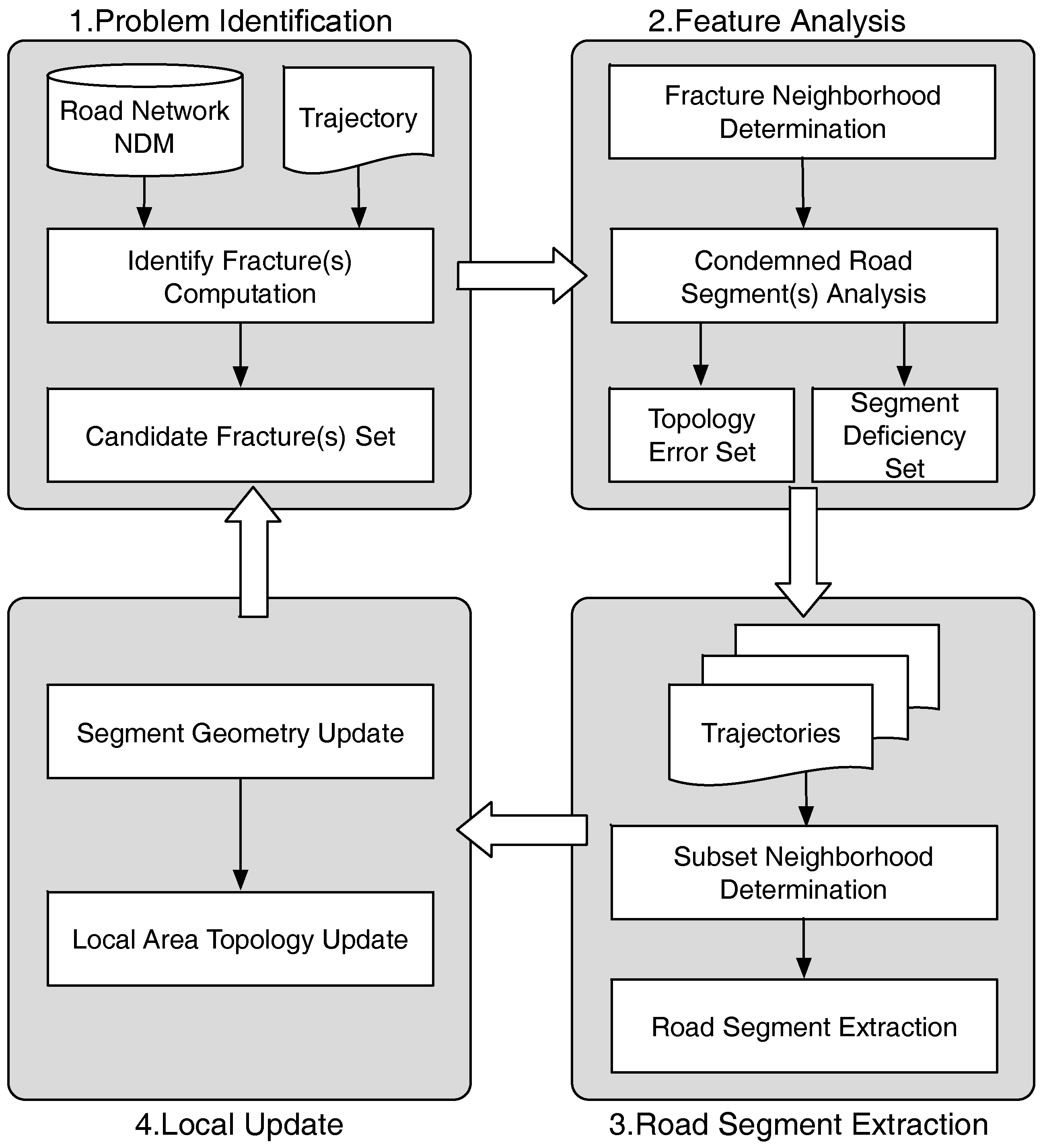
2. A Spiral Inspection and Renewal Strategy

Our work was motivated by the idea of developing an approach that can be utilized to smooth exceptions during matching individual vehicle trajectories. These exceptions made us focus on the problems of road network data, such as topological errors and road segment deficiencies. Since a collection of trajectory data intrinsically includes more information than sequences of spatiotemporal points, we could reconstruct the geometries of the road segments. With that in mind, the first step in this paper is to design an upward spiral updating strategy, which allows us to renew the road network data following the progressive process of “Inspecting >> Analyzing >> Extracting >> Updating”. Such a strategy must be recursively incremental, namely, updating the information of local road networks upon the advent of new problems, as it is relatively flexible to inspect partial road networks with a certain given trajectory. A major challenge of our attempt is to process all the data into a road network because it covers massive amounts of tracking data. Our strategy is to extract the geometry of the subsections of the road network in which there are problems detected. However, the road network reconstruction depends on the quantity and quality of local trajectories to some extent, as we will see in Section 5, especially at locations with less traffic flow or when the offset value of the trajectory is excessive.

2.1. Problem Statement

Before introducing the strategy, we will introduce the preliminaries and formally define the problem of road network data.

Definition 1 (Road Network).

A road network is a directed graph G = (V, E, C) embedded in R², where V ∈ R² is a collection of graph nodes described by two coordinates: longitude and latitude, E ∈ V × V are the directed edges that correspond to road segments (or rs for short) linking two nodes and C ⊂ E × E specifies certain additional limitations (or may be empty), such as transit time costs between adjacent road segments.

As in many typical map sources, e.g., the OSM project, the geometry of roads in this paper is represented by straight road segments, where a curved road can be approximated as a sequence of connected road segments, as illustrated in Figure 1. For simplicity, all nodes are called segment nodes (SNs), although some are not intersections of multiple roads. For instance, the white points in Figure 1 (e.g., SN₁–SN₄) are intersections at road junctions, while the thick points (i.e., SN₅–SN₉) are located on a single road. The accuracy of any operation on a road network also depends on the granularity of the road segments.

Definition 2 (Trajectory).

A trajectory is the path of a moving object captured as a time-stamped series of location points with a certain time interval, denoted as T = (P_i | i = 1, 2, …, n), where P_i = (P_i latitude, P_i longitude, P_i timestamp).

Definition 3 (Road Segments Topology Connectivity Error).

A road segments topology connectivity error is identified if the subsequence of a trajectory T passes through two real road segments, which are discrete in the road network, in succession G. Here, the road segments topology connectivity error is a typical topology error between road segments resulting from the low quality of the primitive metrical road data.

Definition 4 (Road Segment Deficiency).

A road segment deficiency is identified if the subsequence of a trajectory T passes through a real road segment without a corresponding road segment rs in the road network G, which is often due to acquisition of new road information lagging behind urban construction.

The problem of updating road network in this paper is defined as:

Given a set of GPS trajectories and a road network G = (V, E, C), locate the PRS (i.e., road segments topology connectivity error and deficiency) and fix them in the local range.

2.2. Spiral Updating Strategy

The architecture of our proposed updating strategy, as shown in Figure 2, is a spiral progressive process composed of four major stages: Problem Identification, Feature Analysis, Road Segment Extraction, and Local Update. The spiral process breaks the update process into the local areas where every trajectory passes, instead of identifying all PRSs at the very beginning. The strategy processes the whole road network with multiple updating rounds and inspects and updates certain sections of the road network within each round. The number of rounds depends on the input trajectories of the Problem Identification. This allows us to control the number of rounds by limiting the maximum number of input trajectory datasets or to focus on a certain area by specifying a different trajectory.

Problem Identification This stage considers a road network dataset in the form of an NDM (network data model, S. Rogers, et al. 1999 [28]). It accepts a single trajectory from the given trajectory dataset and retrieves all positions of possible PRSs along the trajectory by means of the HMM. This can be efficiently performed with an appropriate HMM combining the road network and the trajectory. The output of this stage is a sequence of candidate GPS point sets (called fracture) indicating the positions of the PRSs.

Feature Analysis This stage determines the neighborhood(s) of the retrieved PRS(s) followed by characteristic and type analysis of the problems. The problems are divided into two sets of problem segments as the output in accordance with the road segments topology connectivity error and road segment deficiency. The results are used later to determine the required partial trajectory data acquisition for extraction and local network update.

• The determination of the neighborhood(s) of PRS(s) considers not only the position information of the corresponding candidate points but also takes account of the distance from the candidate points of the first sampling point to the candidate points of the final sampling point in a fracture. To avoid involving massive amounts of trajectory data in the later computation, we employ the Euclidean distance to determine the range of each neighborhood.
• Characteristic and type analysis measures the transition probabilities in the HMM, great circle distances and the actual average speeds between neighboring points falling into the neighborhood(s) built above. It then compares these values with regular constraints on relative path(s).

Road Segment Extraction This stage extracts road segment information from subset(s) of multiple trajectories against the neighborhood(s) of the retrieved PRS(s). It inputs trajectories relevant to the problem neighborhood(s) and then extracts parts of the trajectory points inside these neighborhood(s) to generate the geometry of the PRS(s). The output of this stage is two sets of road segments.

Local Network Update This stage updates the road network using the road segment information assigned during feature analysis and road segment extraction. It adapts the architecture of the current road network in the local context of each PRS. The results are then used in the next iteration or stored in a database for external studies and applications.

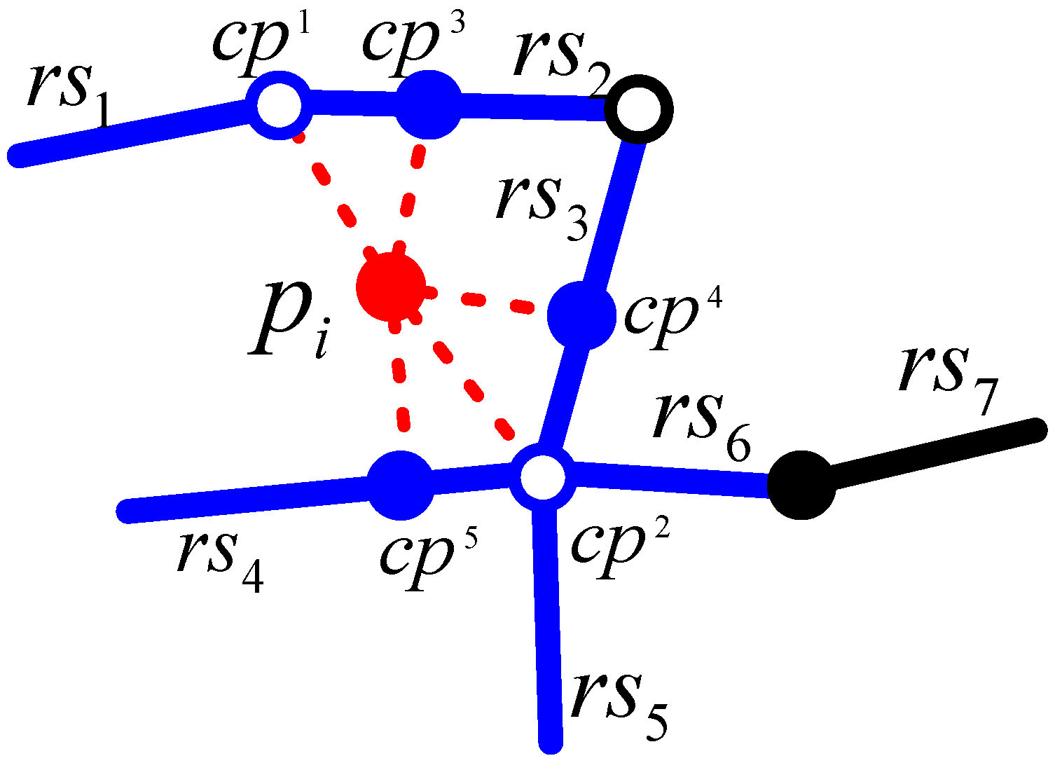
3. The HMM-Based PRS Detection Algorithm

In this section, we describe our HMM-based PRS detection algorithm in detail. The algorithm comprises three basic operations organized into an upward spiral (see Figure 2). Firstly, a set of candidate positions with radius r is retrieved, along with projections of each point P_i along a preprocessed trajectory T. Then, the trajectory T is interpreted to move according to a hidden Markov process on the candidate positions set. Finally, the HMM process is analyzed by detection algorithm, IdentifyFracture, for possible problems in the local area passed by T. In the next processing step, PRSs are marked as a series of deficient positions in the road network for follow-up work. If no problems are detected, the next trajectory is inputted for detecting.

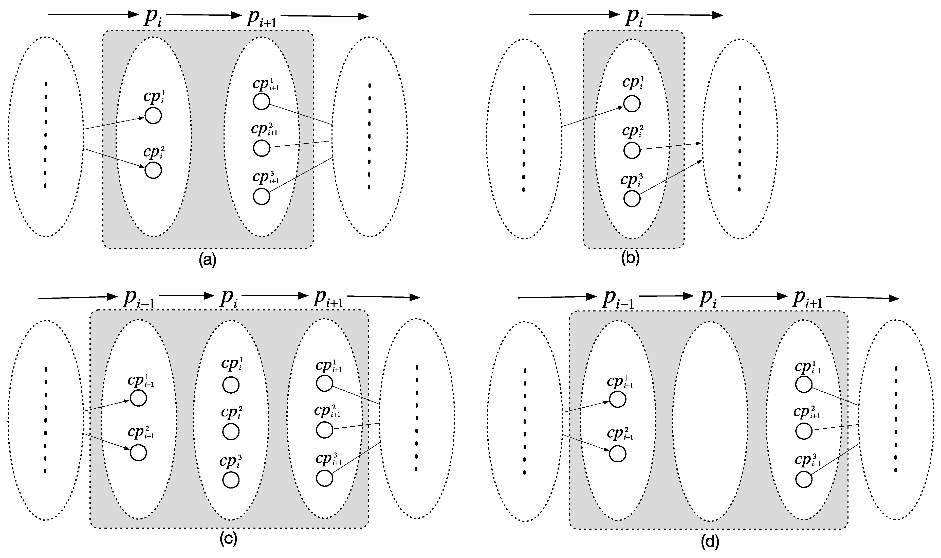
3.1. Candidate Position Preparation

Given the trajectory T = p₁ → p₂ → … → p_n, we first compute all candidate positions in the network corresponding to each point p_i, 1 ≤ i ≤ n, which represents the minimum distance from point p_i to a neighboring road segment rs_j. The candidate position (cp, for short) of point p_i on a road segment rs_j is the projection proj(p_i, rs_j) of point cp onto rs_j:

$$proj(p_i,r{s}_j)=\underset{cp\in r{s}_j}{\arg \min gc(p_i,cp)}$$

(1)

where gc(p_i, cp) is the great circle distance between p_i (the observed point) and points on rs_j. The projection of a sampling point can be either a segment node or a vertical projection point inside a road segment.

It is not realistic to compute candidate positions from all road segments in a network. Instead, thresholds, such as distance r and number k, are employed to limit the calculation of the candidate positions set of p_i on nearby road segments, denoted as CPs(p_i, G, r, k). As shown in Figure 3, the five nearest candidate positions of p_i range from cp¹ to cp⁵, including both segment nodes (cp¹ and cp², related to rs₁, rs₅, and rs₆) and vertical projection points (cp³, cp⁴, and cp⁵, related to rs₂, rs₃, and rs₄, respectively).

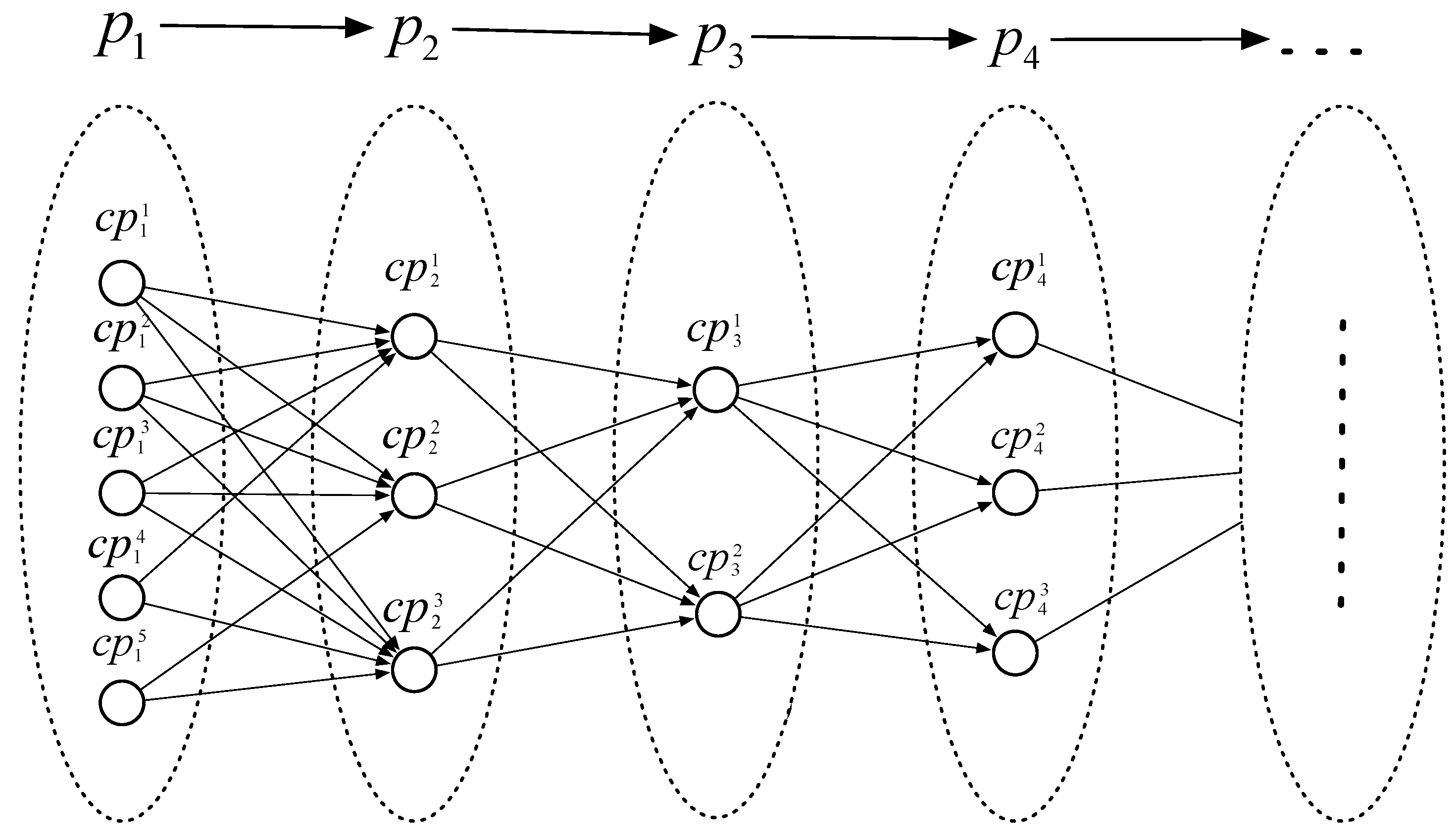
3.2. HMM for Problem Detection

Once all the candidate positions sets along a trajectory T are retrieved, we build the corresponding HMM to detect the underlying problems in the road network. In the ideal first-order HMM for problem detection, the trajectory of a moving object is modeled to move according to a Markov process between discrete candidate positions from the corresponding road segments, which to some extent, is similar to the map-matching approaches of Paul Newson et al. [16]. In addition to incurring the sequence of observations (the path of T), the transition of hidden states (candidate positions) can reflect, from the perspective of HMM, the structure of the local road network that it passes over from the side. That is, problems in the road network data could be marked when we focus on possible fractures during the hidden state Markov process. However, the emission probabilities and state transition probabilities are given before the detection algorithm is introduced because they are the basic components of the HMM.

Emission Probabilities These probabilities give the likelihood of obtaining a sampling point p given a candidate position cp on a road segment rs, denoted as pr(p|cp). Since the GPS noise can be assumed to obey the Gaussian distribution, based on previous work (Paul Newson et al., 2009 [16]), we formally define the emission probability pr(p|cp) as:

$$\mathrm{Pr}(p|cp)=\frac{1}{\sqrt{2\pi \sigma }}\exp {\left(\frac{\Vert p-cp\Vert gc}{\sqrt{2\sigma }}\right)}^2$$

(2)

where ‖p − cp‖gc is the great circle distance between the sampling point p and a candidate position cp. The parameter σ is the standard deviation of the GPS measurement.

State Transition Probabilities These probabilities give the likelihood of the real path of trajectory T from one candidate position cp_i to another candidate position cp_j, which corresponds to two successive sampling points on T. The probabilities are normalized to be proportional to the transit time between the candidate positions on the road network by applying the following formula:

$$\mathrm{Pr}(p_{k+1}\to c{p}_j|p_k\to c{p}_i)\propto \frac{1}{\beta }\exp \left(-\frac{\Vert t_{∆}-t_{\arg }\Vert }{\beta }\right)$$

(3)

where t_∆ denotes the true transit time cost from the former observed point p_k to the next point p_k+1, and t_arg denotes the average transit time cost from cp_i to cp_j extracted from historical statistics. β is a parameter to control the effect of the average transit time. The transit time (or driving time) between two candidate positions is introduced to the transition probability computation in this paper instead of the route distance used in previous work (Rudy Raymond et al., 2012 [34]) because the real transit time of non-specific vehicles more accurately describes the normal conditions of movement through a certain path that is the transition from a candidate position to another in our HMM.

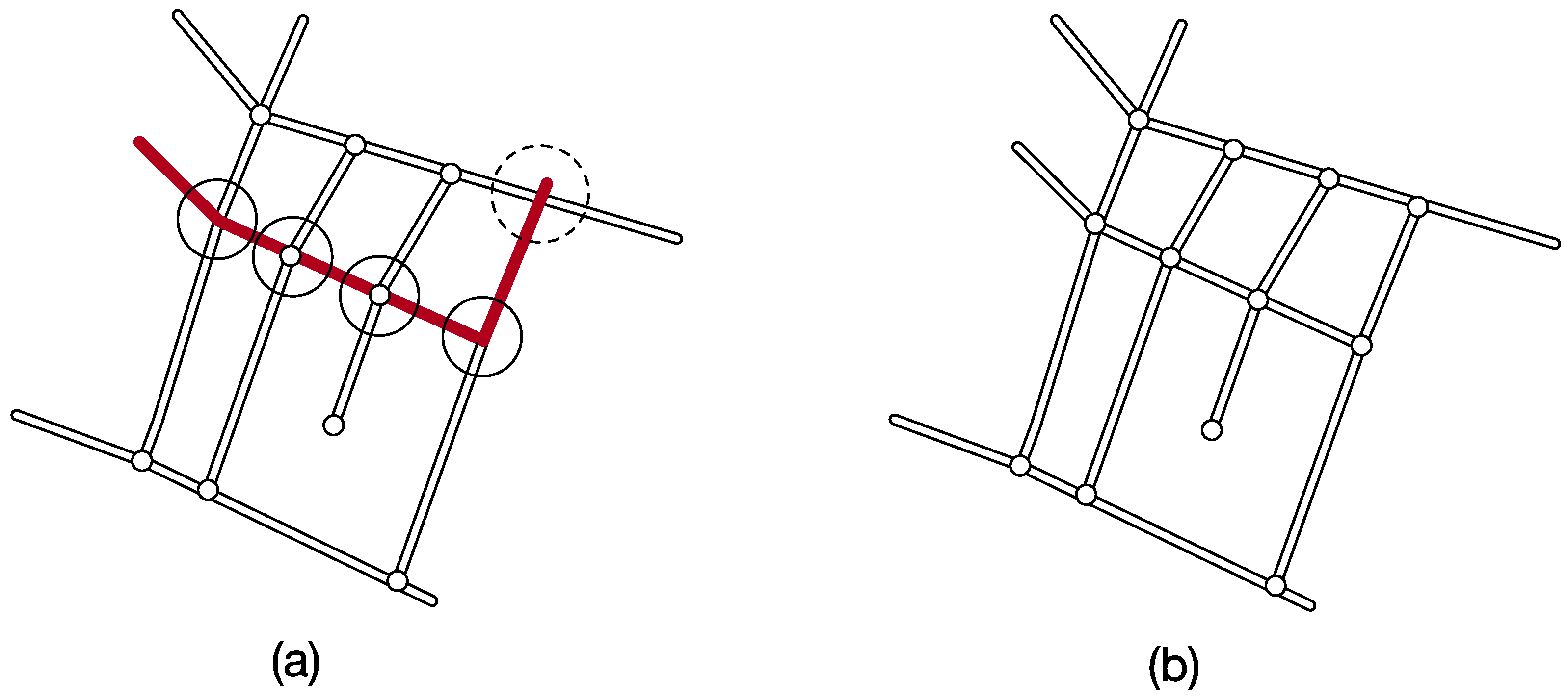
3.3. Problem Detection

With the probabilities above, we design our detection algorithm to identify problem segments along the Markov process composed by candidate positions. The identification process begins with the input of a trajectory T and generates an HMM graph G′ (as shown in Figure 4) after all candidate positions on the road network G and probabilities are calculated. Then, problems with road segments inside the path of T are marked when checking the HMM graph along T.

The HMM graph for T, denoted as G′ = (V′, E′), represents the candidate positions set of all sampling points (denoted as V′) and the set of probable subpaths between two successive sampling points (denoted as E′). In this way, we can take T in G′ as the path that best matches its sample points sequence, although the optimal path is not a concern for us in this paper. PRSs inside the path of T are thus captured as fractures on the related subpaths where the probabilities (either emission probabilities or state transition probabilities) from the candidate points of one sampling point to the next sampling point in G′ are infinitesimally small (approximately zero). For instance, cp_i and cp_j are the candidate potions of two sampling points (p_i and p_j) on two detached road segments in G, which are connected in the real world. Then, a fracture can be identified by an infinitesimally small state transition probability in G′, if p_i and p_j are successive with respect to sampling time.

Algorithm IdentifyFracture

Input: The candidate position sequence CPs, Road network G.

Output: The fracture sequence F in G

1: G′ = GenerateHMMG(G,CPs); // generates HMM graph G’

2: Initialize F as an empty list; // a sequence of fractures

3: Initialize f as an empty fracture; // a container of fractures

4: for each sampling point pi do

5:          if cp set of pi is empty then add pi to f;

6:                 continue;// moves to the next sampling point

7:          if no subpath from cp set of pi to next is available then add pi to f;

8:                 continue;// moves to the next sampling point

9:          if no cp of pi both connects subpaths on two sides then

10:                if pi is not endpoint of trajectory then add pi to f;

11:         if the fracture is not empty then push f into F and clear f;

12: return F;

The algorithm, IdentifyFracture, is introduced to detect all fractures throughout the trip of T. We first construct the graph G′ = (V′, E′) by building HMM on the candidate position sequence CPs. Then, we check on the connectivity of G′ by searching for fractures between candidate positions and subpaths along the topological order of the graph. Finally, the fracture sequence F, consisting of sampling points in the form of tuples (p_s, p_e), whose elements are the starting and ending points of a fracture, respectively, is reported.

The algorithm first checks whether the candidate position set of the sampling point p_i is empty and then determines the subpaths from the candidate positions of p_i to the candidate positions of the next sampling point p_i+1. If the sampling point p_i fails to pass the check, it is assigned to p_s if p_s is empty, otherwise the next sampling point p_i+1 is assigned to p_e (as shown in Figure 5a). There is one important exception: when both candidate positions and subpaths of p_i (which is not the first or last point of a trajectory) are available but none of the candidate positions connects the subpaths on either side. In this case, the point is assigned to both p_s and p_e (as shown in Figure 5b). Once a sampling point p_i passes the check and p_s and p_e are not empty, a fracture in the form of (p_s, p_e) is added to F, and p_s and p_e are cleared. The value of p_s cannot be changed after the assignment until it is cleared, while the value of p_e may be replaced before it is cleared. For example, Figure 5 presents four types of fractures identified by the algorithm IdentifyFracture. The p_e in Figure 5c,d was assigned to p_i and then replaced by p_i+1.

4. Local Road Segments Extraction and Updating

Given the fractures in the previous section, we can locate the sampling points to determine the locations of problems and explore a method to reconstruct road segments using multiple trajectories collected by non-specialized vehicles or persons. We can repair PRSs and connectivity on the local scale. The first step is to build the neighborhood of each problem, which defines the local area that is involved and helps to analyze characteristics of the problem. The next step is concerned with new trajectories related to the neighborhood and consists of two tasks: (1) generating the geometries of the new road segments; and (2) updating the geometry of the road segments. The details of these steps are described in the following.

4.1. Problem Neighborhood

The neighborhood of a problem is determined by the fracture’s start and end (p_s and p_e), as well as the candidate positions, which produces a circular area with the longest distance between candidate positions of p_s and p_e as the diameter. For instance, in Figure 6, the trajectory T = p₁ → p₂ → … → p₆ encounters a fracture that indicates a problem in G. The red dots represent the sampling point passing detection, and the grey dots mark the sampling points of the fracture (i.e., p₃, p₄ and p₅). The neighborhood is determined by the candidate points of the fracture’s start (p_s = p₃) and end (p_e = p₅).

After the problem neighborhood is built, we can address the related PRSs. First, the connectivities between the original road segments inside the neighborhood are examined. The neighborhood’s diameter is compared to a distance threshold to determine whether it is a topology error or a segment deficiency. Topology errors can be corrected by operations such as “stretch” and “merge”, while missed segments are recovered later by geometries extracted from multiple trajectories.

4.2. Road Segment Extraction

The objective of this step is to generate the geometry of the missed road segments to reconstruct the local road network. For practical purposes, the subsection of a single trajectory on the local area is often relatively sparse and fails to provide sufficient spatial information. We thus tend to extract geometry from multiple relevant trajectories in the problem neighborhood.

A clustering method is introduced to group all sampling points and to find skeleton points that represent the underlying road segments in view of the low complexity of the road segments inside a problem neighborhood. Our assumptions are that the all input sampling points sequences follow a similar path inside the problem neighborhood as the trajectory for problem detection. This would require a preprocessing to filter multiple trajectories in a neighborhood based on speed and direction angle for the sake of a unique path. However, we focus on describing the methods of road segment extraction in this section due to the limited capacity.

We selected PAM (partitioning around medoids [33]) from a wide variety of clustering methods due to its robustness to noise and outliers and its effectiveness and efficiency on a small dataset. The sampling point of the trajectories were grouped into clusters following the road segment skeletons using the PAM method, which produced a relatively good clustering structure by minimizing the geometric distance between sampling points. PAM aims to divide all sampling points into clusters by iteratively swapping the dissimilarities from all points to the nearest medoid. The PAM extracting skeletons for the segments has three steps:

(1)

determining a suitable number of clusters (k) by means of “Silhouettes” [32] after obtaining the subsections of multiple trajectory data inside the problem neighborhood;

(2)

randomly selecting k sampling points as the initial medoids and iteratively checking whether any medoid needs to be replaced by calculating the dissimilarities between the unselected points and medoids;

(3)

reducing all medoids by thresholds, such as the steering angle and distance, and connecting the remaining medoids in sequence.

4.3. Local Road Segments Updating

The last step is to update the geometry and topology information in a partial area of the original road network. We first add the generated segments to the original, followed by updating the topology using two operations: (1) renewing intersections and (2) connecting road segments.

Renewing intersections This operation identifies intersection relationships between the generated segments and the original segments nearby. If there are intersection relationships, then new intersections are generated to further split the segments. An intersection relationship is identified if the angles between two segments is greater than 30° and one of them crosses the other (marked by solid circles in Figure 7a).

Connecting road segments It is import to ensure the connectivity between generated the segments and original segments. If there are any gaps (marked by dotted circles in Figure 7a, the segments will be extended to the adjacent original segments along the shortest distance.

5. Experiments

To validate the proposed method, we perform sets of experiments using real data in this section. We first present the experimental setting, including the dataset used and certain parameters. Then, we report the major testing results followed by discussions. All the experiments are implemented in Visual Studio based on ArcGIS 10.3 with an Intel Core Quad CPU i7 2.30GHz machine with 8 GB of memory running Microsoft Windows 8.1.

5.1. Experimental Setting

Dataset Description The road network data of Wuhan, which covers roads ranging between 113°41′ and 115°05′ longitude and 29°58′ and 31°22′ latitude, were taken directly from OSM’s website. From the available trajectory dataset collected through the GPS devices of taxies, a total of 36 continuous filtered trajectories were obtained from the original dataset in Wuhan on 29th May 2014, and confirmed to be located adjacently in space. We filtered the raw GPS trajectories (in GPX format) based on the following conditions: (1) the number of satellites available during data collection was more than 4; (2) the sampling period ranged from 30 to 60 s; (3) the average horizontal dilution of precision (HDOP) was less than 1.25. The motivation behind the filtering is to eliminate outliers and redundancies in trajectory dataset. Six trajectories were randomly selected from the 36 trajectories as inputs to the detection algorithm, while all 36 trajectories were used as inputs for the road segment extraction and updating.

Parameters for Problem Detection Five parameters are needed in our detection algorithm, including the candidate retrieve radius r and the maximum number of candidate positions k. The candidate retrieve radius r is set to 200 m, as in many map-matching approaches (e.g., [33,34,35]), which means the emission probability from a GPS point to any road segment is zero if they are 200 m (or more) apart. Then, we estimated the impact of the maximum number of candidate positions k on the average detection accuracy and average running time of the detection algorithm for the maximum number of candidate positions. The detection accuracy continuously increases as more candidate positions are considered (as shown in Figure 8a). However, more using candidate positions for each GPS sampling point would result in increased computation on more road segments, which would increase the running time. As shown in Figure 8b, the running time is relatively acceptable when we k = 4. Thus, we use k = 4 for the sampling points. For the HMM probabilities estimation, we employ a normal distribution with δ = 20.0 m for the emission probability and β = 100.0 for the state transition probability.

Baseline and Evaluation Approach The road network baseline was generated manually using high-resolution and original OSM road network data, as well as editing tools in ArcGIS 10.3. The 0.6 m pixel resolution satellite imagery for Wuhan City obtained from Tianditu (a public map service released in 2013 by the National Geomatics Center of China) was employed as a backdrop. To measure the accuracy of the baseline, the sample ground truth positions (i.e., junctions) in Wuhan’s main urban area were collected using a vector map of Wuhan, 2013, from NGCC (National Geomatics Center of China). The difference between reference points and the digitized points is on average 1.76 m, with a standard deviation of 0.89 m.

We evaluate the performance of our method in terms of the road segment quality. The measurements of road segment quality include both qualitative determination and quantitative metrics proposed by Wiedemann [36]. The quantitative metrics cover geometry and topology, respectively, which are defined as follows:

$$M_{geometry}=\frac{{\displaystyle \sum \mathrm{The}\mathrm{length}\mathrm{of}\mathrm{generated}\mathrm{road}\mathrm{segments}\mathrm{matched}\mathrm{reality}}}{{\displaystyle \sum \mathrm{The}\mathrm{length}\mathrm{of}\mathrm{generated}\mathrm{road}\mathrm{segments}}}$$

(4)

$$M_{topology}=\frac{{\displaystyle \sum \mathrm{The}\mathrm{number}\mathrm{of}\mathrm{generated}\mathrm{intersections}\mathrm{matched}\mathrm{reality}}}{{\displaystyle \sum \mathrm{The}\mathrm{number}\mathrm{of}\mathrm{generated}\mathrm{intersections}}}$$

(5)

A generated road segment matches the baseline if the longest projection distance from it to the baseline satisfies a distance threshold (called the buffer distance). In this paper, the threshold is set to 3.75 m, the minimum width for a road according to the Wuhan Traffic Management Bureau.

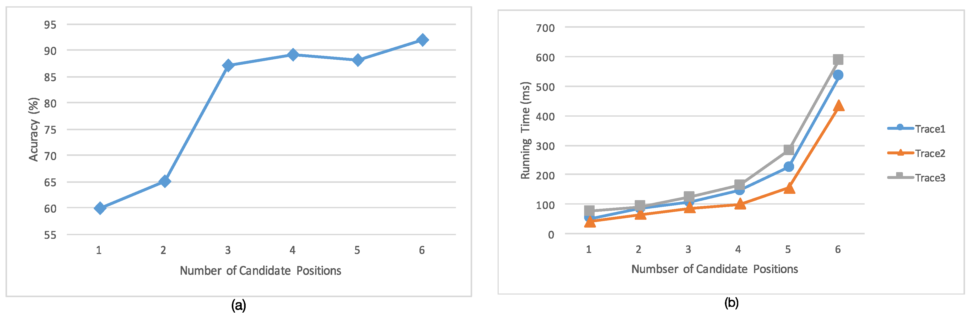
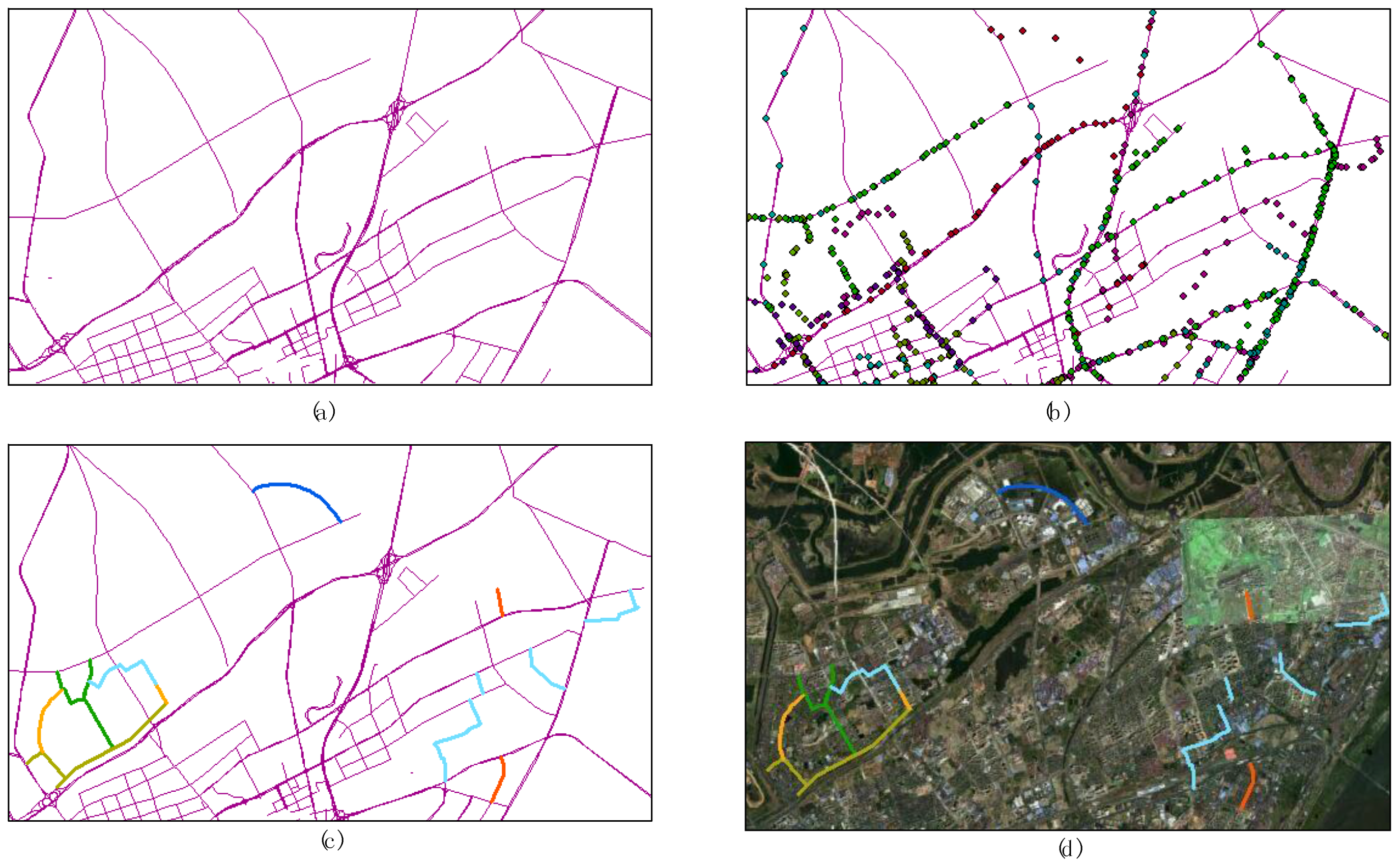
5.2. Experimental Results

Wuhan has been building out and renewing the road network of its urban area in recent years. Several new roads have been completed and opened to traffic. The geographic areas passed by these trajectories contain several new roads or reconstructed roads, which were our primary targets in updating the road network. Figure 9a,b show the updated road segments in our experiment. As shown in these figures, six trajectories were selected as the input trajectories for the detection algorithm and six rounds of updating were performed, while the other trajectories were used for road segment extraction. These changes were not identified and updated all at once. Instead, the network was inspected by the IdentifyFracture algorithm each time a trajectory was inputted, followed by extracting and updating using the whole trajectory dataset, i.e., the progressive process of “Inspecting >> Analyzing >> Extracting >> Updating” was executed in six rounds.

During the six rounds, a total of 12 fractures were identified by HMM and were updated within the corresponding problem neighborhoods. With each round of the spiral process, once the fractures in the HMM graph were found, they were used as the input to construct the problem neighborhoods. Then, sampling points failing in the new problem neighborhoods were used to generate new segments or to adjust existing segments. Figure 9c,d show the results of the six rounds of road network updating compared to the original network and RS images. Lines with six different colors represent the generated segments obtained from the related trajectories. It is intuitively plausible to see that the updated road network, to a certain degree, matches the roads in the real world when compared to the RS image (as shown in Figure 9d).

We calculated M_geometry and M_topology after each round of the updating process. As shown in

Table 1. Quality measures of the updating experiment.

	Round 1	Round 2	Round 3	Round 4	Round 5	Round 6
Mgeometry	75.5%	88.5%	88.5%	85.8%	87.4%	86.6%
Mtopology	80%	77.8%	66.7%	75%	66.7%	76.9%

, the M_geometry of the updated road network, as expected, depends heavily on the quality of the GPS trajectories, just as all road network construction or reconstruction approaches do. The M_topology of the updated network is strongly impacted by the complexity of the local network structure. The updated network in the first round (indicated by the dark blue line in in Figure 9c) has a lower M_geometry than those in the other rounds, and it has a higher M_topology than the others. This is because a new road was constructed, and it was less traveled by vehicles. The local network structure in the problem neighborhood is relatively simple despite the sparse trajectory data. However, the M_topology of rounds 3 (indicated by green lines) and 5 (indicated by light blue lines) is lower due to their more complicated local network structures.

Additionally, the M_topology values are generally not sufficient, although they are acceptable. That is because we directly extended segments along the shortest distance to eliminate gaps between road segments, which does not always correspond to reality. The quality of the raw trajectory data is also important with respect to this issue. For example, the collected trajectory data are sparse in the area or are interrupted by buildings nearby. We plan to blunt these negative effects by using new approaches to reconstruct road network topology in subsequent research work.

The quality of the updated results was also compared to the approach in [16]. The average M_geometry of the approach in [16] (denoted by AhmedM) was lower than reported because we did not execute preprocessing steps. Figure 10 shows that the average M_geometry in our results is relatively stable. In other words, the result of our method (denoted by SpiralM) does not heavily depend on massive trajectory data. This could be because the method in this paper processes only the PRS s on the foundation of the existing road network and computes only the sampling points inside the neighborhoods of these PRS s, whereas in the other method, all road geometries were re-generated. Each round of our spiral updating could make use of the output of the previous round. By having fewer trajectories for the computation, we could achieve a relatively accurate result by refining the existing road network. However, the gap between the two methods narrowed as we added additional trajectories to the dataset used in the experiment.

6. Conclusions

In this paper, we investigated the problem of updating road networks at the local scale using trajectory data. Our proposal is based on an HMM-based PRS detection algorithm, upon which a new spiral strategy was derived to inspect and update an existing road network through potential path information from non-specialized vehicle traces. The spiral strategy was designed following the progressive process of “Inspecting >> Analyzing >> Extracting >> Updating.” It starts from an HMM-based algorithm and automatically detects and analyzes missing road segments and topological errors and continues extracting road segments from multiple trajectories in the local context of locations that failed the detection process, eventually updating the original road network in the local area.

To facilitate the updating framework, we also redesigned the HMM graph consisting of a sampling point sequence and the corresponding candidate positions following the ideal HMM. Further, we developed an algorithm to find fractures inside the HMM graph, which helped us to locate problem road segments in the road network. Then, we constructed a neighborhood for each PRS and extracted the geometry information from the subsections of multiple trajectories to update the road network. These processes were validated by experiments using real data. To the best of the authors’ knowledge, this study is the first attempt to check existing road network structures and to renew them from the local to whole scale by means of massive numbers of GPS vehicle trajectories.

In the near future, in addition to continuing to explore algorithms for detecting problems and reconstructing local road networks, we will investigate three related research issues raised by this string-expressed model. The first is to improve the spiral updating strategy in a more robust way. The second is to design new approaches to extract road segment information from a small set of trajectory data. This will help to automatically maintain and update the existing road network data with less cost and can therefore be used to generate new road networks more conveniently and efficiently.

References

1. Fusco, S.J.; Michael, K.; Michael, M.G. Using a social informatics framework to study the effects of location-based social networking on relationships between people: A review of literature. In Proceedings of the IEEE International Symposium on Technology and Society (ISTAS’10), Wollongong, Australia, 7–9 June 2010.
2. Karimi, H.A.; Zimmerman, B.; Ozcelik, A.; Roongpiboonsopit, D. SoNavNet: A framework for social navigation networks. In Proceedings of the International Workshop on Locations Based Social Networks (LBSN’09), Seattle, WA, USA, 4–6 November 2009.
3. Haklay, M.; Weber, P. OpenStreetMap: User-generated street maps. IEEE Pervasive Comput. 2008, 7, 12–18. [Google Scholar] [CrossRef]
4. Porikli, F. Road extraction by point-wise Gaussian models. Proc. SPIE 2003. [Google Scholar] [CrossRef]
5. Li, X.; Zhang, S.; Pan, X.; Dale, P.; Cropp, R. Straight road edge detection from high-resolution remote sensing images based on ridgelet transform with revised parallel-beam radon transform. Int. J. Remote Sens. 2010, 31, 5041–5059. [Google Scholar] [CrossRef]
6. Unsalan, C.; Sirmacek, B. Road network detection using probabilistic and graph theoretical methods. IEEE Trans. Geosci. Remote Sens. 2012, 50, 4441–4453. [Google Scholar] [CrossRef]
7. Doucette, P.; Agouris, P.; Stefanidis, A.; Musavi, M. Self-organised clustering for road extraction in classified imagery. ISPRS J. Photogramm. Remote Sens. 2001, 55, 347–358. [Google Scholar] [CrossRef]
8. Shi, W.; Miao, Z.; Wang, Q.; Zhang, H. Spectral-spatial classification and shape features for urban road centreline extraction. IEEE Geosci. Remote Sens. Lett. 2014, 11, 788–792. [Google Scholar]
9. Mumtaz, S.A.; Kevin, M. Fusion of high resolution LiDAR and aerial images for object extraction. In Proceedings of the 2nd International Conference on Advances in Space Technologies, Islamabad, Pakistan, 29–30 November 2008; pp. 137–142.
10. Fang, L.; Yang, B. Automated extracting structural roads from mobile laser scanning point clouds. Acta Geod. Cartogr. Sin. 2013, 42, 260–267. [Google Scholar]
11. Lee, Y.; Cho, S.B. Extracting meaningful contexts from mobile life log. In Lecture Notes in Computer Science; Springer: Berlin, Germany, 2007; pp. 750–759. [Google Scholar]
12. Zheng, Y.; LI, Q.; Chen, Y.; Xie, X.; Ma, W. Understanding mobility based on GPS data. In Proceedings of the 10th International Conference on Ubiquitous Computing (UbiComp’08), Seoul, Korea, 21–24 September 2008.
13. Efentakis, A.; Brakatsoulas, S.; Grivas, N.; Lamprianidis, G.; Patroumpas, K.; Pfoser, D. Towards a flexible and scalable fleet management service. In Proceedings of the ACM Sigspatial International Workshop on Computational Transportation Science, Orlando, FL, USA, 5–8 November 2013; pp. 79–84.
14. Brakatsoulas, S.; Pfoser, D.; Salas, R.; Wenk, C. On map-matching vehicle tracking data. In Proceedings of the 31st VLDB Conference on Very Large Data Bases, Trento, Italy, 4–6 October 2005; pp. 853–864.
15. Guo, T.; Iwamura, K.; Koga, M. Towards high accuracy road maps generation from massive GPS traces data. In Proceedings of the IEEE International Geoscience and Remote Sensing Symposium (IGRASS’07), Barcelona, Spain, 23–28 July 2007; pp. 667–670.
16. Ahmed, M.; Wenk, C. Constructing street networks from GPS trajectories. In Proceedings of the 20th Annual European Symposium on Algorithms, Ljubljana, Slovenia, 10–12 September 2012; pp. 60–71.
17. Ahmed, M.; Karagiorgou, S.; Pfoser, D.; Wenk, C. A comparison and evaluation of map construction algorithms using vehicle tracking data. Geoinformatica 2015, 19, 601–632. [Google Scholar] [CrossRef]
18. Edelkamp, S.; Schroedl, S. Route planning and map inference with global positioning traces. In Computer Science in Perspective: Essays Dedicated to Thomas Ottmann; Springer-Verlag: New York, NY, USA, 2003; pp. 128–151. [Google Scholar]
19. Schroedl, S.; Wagstaff, K.; Rogers, S.; Langley, P.; Wilson, C. Mining GPS traces for map refinement. Data Min. Knowl. Discov. 2004, 9, 59–87. [Google Scholar] [CrossRef]
20. Worrall, S.; Nebot, E. Automated process for generating digitized maps through GPS data compression. In Proceedings of the 2007 Australasian Conference on Robotics and Automation Brisbane, Brisbane, Australia, 10–12 December 2007.
21. Chen, C.; Cheng, Y. Roads digital map generation with multi-track GPS data. In Proceedings of the 2008 International Workshop on Geoscience and Remote Sensing, Washington, DC, USA, 21–22 December 2008.
22. Shi, W.; Shen, S.; Liu, Y. Automatic generation of road network map from massive GPS vehicle trajectories. In Proceedings of the 12th International IEEE Conference on Intelligent Transportation Systems, St. Louis, MO, USA, 4–7 October 2009; pp. 48–53.
23. Cao, L.; Krumm, J. From GPS traces to a routable road map. In Proceedings of the Workshop on Advances in Geographic Information Systems, Seattle, WA, USA, 4–6 November 2009.
24. Fathi, A.; Krumm, J. Detecting road intersections from GPS traces. In Lecture Notes in Computer Science; Springer: Berlin/Heidelberg, Germany, 2010; pp. 56–69. [Google Scholar]
25. Kasemsuppakorn, P.; Karimi, A.H. A pedestrian network construction algorithm based on multiple GPS traces. Transp. Res. Part C 2013, 26, 285–300. [Google Scholar] [CrossRef]
26. Biagioni, J.; Eriksson, J. Map inference in the face of noise and disparity. In Proceedings of the International Conference on Advances in Geographic Information Systems, Redondo Beach, CA, USA, 7–9 November 2012.
27. Karagiorgou, S.; Pfoser, D.; Skoutas, D. Segmentation-based road network construction. In Proceedings of the International Conference on Advances in Geographic Information Systems, Orlando, FL, USA, 5–8 November 2013.
28. Rogers, S.; Langley, P.; Wilson, C. Mining GPS data to augment road models. In Proceedings of the International Conference on Knowledge Discovery and Data Mining, San Jose, CA, USA, 15–18 August 1999.
29. Zhang, L.; Thiemann, F.; Sester, M. Integration of GPS traces with road map. In Proceedings of the International Conference on Advances in Geographic Informatics Systems (ACM SIGSPATIAL’10), San Jose, CA, USA, 3–5 November 2010.
30. Li, J.; Qin, Q.; Xie, C.; Zhao, Y. Integrated use of spatial and semantic relationships for extracting road networks from floating car data. Int. J. Appl. Earth Obs. Geoinform. 2012, 19, 238–247. [Google Scholar] [CrossRef]
31. Rabiner, L.; Juang, B. An introduction to hidden Markov models. IEEE ASSP Mag. 1986, 3, 4–16. [Google Scholar] [CrossRef]
32. Kaufman, L.; Rousseeuw, P.J. Clustering by means of medoid. In Statistical Data Analysis Based on the L1 Norm; Dodge, Y., Ed.; Elsevier/North-Holland: Amsterdam, the Netherlands, 1987; pp. 405–416. [Google Scholar]
33. Newson, P.; Krumm, J. Hidden markov map matching through noise and sparseness. In Proceedings of the International Conference on Advances in Geographic Informatics Systems (ACM SIGSPATIAL’09), Seattle, WA, USA, 4–6 November 2009.
34. Raymond, R.; Morimura, T.; Osogami, T.; Hirosue, H. Map matching with hidden Markov model on sampled road network. In Proceedings of the 21st International Conference on Pattern Recognition (ICPR 2012), Tsukuba, Japan, 11–15 November 2012.
35. Szwed, P.; Pekala, K. An incremental map-matching algorithm based on hidden Markov model. In Proceedings of International Conference on Artificial Intellifence and Soft Computing, Zakopane, Poland, 1–5 June 2014; pp. 579–590.
36. Wiedemann, C. External evaluation of road networks. ISPRS Arch. 2003, 34, 93–98. [Google Scholar]
Figure 1. Representing road network data by nodes and segments.
Ijgi 05 00163 g001
Figure 2. Overview of the updating strategy.
Ijgi 05 00163 g002
Figure 3. Candidate positions of sampling point pi on neighboring road segments.
Ijgi 05 00163 g003
Figure 4. The HMM graph G′.
Ijgi 05 00163 g004
Figure 5. Four types of fractures in G′: (a) the fracture between two sequential sampling points; (b) the fracture on one sampling point; (c) a fracture among multiple sequential sampling points; and (d) a fracture among multiple sequential sampling points, in which there is sampling point without any candidate position.
Ijgi 05 00163 g005
Figure 6. A PRS neighborhood in a road network.
Ijgi 05 00163 g006
Figure 7. Updating a road network on the local scale: (a) generated road segments on the original road network; and (b) the updated road network.
Ijgi 05 00163 g007
Figure 8. (a) Accuracy w.r.t. number of candidate positions; and (b) Running time w.r.t. number of candidate positions.
Ijgi 05 00163 g008
Figure 9. Six rounds of the road network updating experiment: (a) the original road network; (b) the input trajectories; (c) the updated road network; and (d) comparison between generated road segments and a satellite map.
Ijgi 05 00163 g009
Figure 10. Comparison of results.
Ijgi 05 00163 g010